二維非複利葉熱傳導問題之正解與逆解之理論與實驗研究

行政院國家科學委員會專題研究計畫 成果報告

二維非複利葉熱傳導問題之正解與逆解之理論與實驗研究

研究成果報告(精簡版)

計 畫 類 別 ： 個別型 計 畫 編 號 ： NSC 94-2212-E-151-019- 執 行 期 間 ： 94 年 08 月 01 日至 95 年 10 月 31 日 執 行 單 位 ： 國立高雄應用科技大學模具工程系 計 畫 主 持 人 ： 楊慶煜 計畫參與人員： 博士班研究生-兼任助理：蕭美枝 碩士班研究生-兼任助理：郭繼仁、王瑞詠 報 告 附 件 ： 出席國際會議研究心得報告及發表論文 處 理 方 式 ： 本計畫可公開查詢

中 華 民 國 96 年 01 月 30 日

行政院國家科學委員會專題研究計畫成果報告

二維非複利葉熱傳導問題之正解與逆解之理論

與實驗研究

計畫編號: 94-2212-E-151-019-執行期限:94 年 8 月 1 日至 95 年 10 月 31 日 主持人: 楊慶煜 國立高雄應用科技大學模具系 中文摘要 逆運算熱傳導問題簡稱為 IHCP， 一 般是應用熱電耦或紅外線光學法量得 固體內部點或表面的溫度值，以反求 邊界條件、熱傳係數、表面熱傳量、 內部熱源等。在過去的逆運算領域的 研究中，多數學者發展的方法僅限於 複利葉熱傳的系統，亦即拋物線型的 熱傳系統。然而在高功率雷射加工、 低溫熱傳工程實際問題中，拋物線型 的熱傳無法描述實際的熱傳現象，意 即熱傳以有限速度傳播，因此必須以 非複利葉熱傳系統，亦即雙曲線型熱 傳方程式來描述。在非複利葉熱傳系 統中由於熱通量與溫度梯度響應不一 致，造成溫度已有限速度傳遞。 過去的研究中，已有所多成果發 表有關一維非複利葉熱傳直接解問 題。Lor and Chu [1] 解析非複利葉 熱阻問題，Antaki [2] 探討非複利葉 固相介面問題，Sanderson and etc. [3] and Liu and etc. [4]研究雷射生成 超音波問題，Mullis [5, 6] 討論快 速凝固問題、Roetzel and Ranong [7] and Roetzel and etc. [8, 9] 計算 非複利葉熱交換器問題，Lin [10], Abdel-Hamid [11], Tang and Araki [12] 解析週期邊界非複利葉問題，Tan and Yang [13, 14]以非複利葉模式探 討薄膜熱傳現象。然而僅有少數的研 究 曾 涉 及 二 維 非 複 利 葉 問 題 [15-16].Yang [15] 發展一空間切割 與無震動的數值方法求解問題。Chen and Lin [16]使用控制容積與拉氏轉 換法求解二維問題。 在本計畫中將推 導一有限差分架構之數值方法求解二 維非複利葉熱傳直接解問題。 比起直接解問題，非複利葉熱傳 逆運算問題的探討並不多，在一維問 題中 Weber [17]使用二階差分方程式 求解問題，Al-Khalidy [18, 19] 採 用控制容積法與空間搜尋法（Space marching method）, Chen and etc. [20] 應用拉氏轉換、控制容積與非線性最 佳化估算邊界。上述研究中，普遍存 在最初估算結 果不穩 定的問題 ， 而 Yang [21]運用未來時間觀念有效解決 此問題。然而截至目前為止並無任何 研究探討二維非複利葉熱傳逆運算問 題，因此本研究中將推導有效且精確 的方法估算二維非複利葉熱傳邊界問 題。 估算非複利葉熱傳問題的邊界， 較複利葉熱傳導系統困難。原因在於 熱傳以有限速度傳送，量測點與被估 物理量所在位置存在時間延遲之現 象，另一個原因為以雙曲線型熱傳以 熱傳波傳遞，求解過程較為複雜。因 此造成此類問題使用上的困難與限 制。也因此發展一精確、穩定與快速 的非複利葉逆熱傳邊界估算方法，為 本計畫預計達成之目標。 關鍵詞: 逆運算，非複利葉熱傳，雙曲 線型熱傳，未來時間

Abstract

The non-Fourier heat transfer

induces thermal waves by delaying the

response between heat flux and

temperature gradient. This delay may

represent time needed to accumulate energy for signification heat transfer

and lead to the thermal wave

propagation with a finite speed. The

mathematical representation for the

non-Fourier effect is a hyperbolic

equation that included a wave

propagation term. The heat transfer

propagates at a finite speed instead of infinite speed that is the Fourier heat

conduction. The non-Fourier effect

becomes more and more attract in practical engineering problems such as the non-homogenous solids conduction process, the rapid heating process, and the slow conduction process [1-14].

The study of the hyperbolic heat conduction problems is fall into two

catalogaries. One is the investigation

of the methods of the direct analysis and

the other is the inverse analysis. Most

researches of the direct analysis are focus on the one-dimensional problems. Lor and Chu [1] analyzed the problem with the interface thermal resistance. Antaki [2] discussed the heat transfer in

solid-phase reactions. Sanderson and

etc. [3] and Liu and etc. [4] investigated the laser generated ultrasound models.

Mullis [5, 6] discussed the rapid

solidification problems. Roetzel and Ranong [7] and Roetzel and etc. [8, 9] calculated the heat exchanger problems. Lin [10], Abdel-Hamid [11], Tang and Araki [12] computed the non-Fourier fin problems under the periodic thermal conditions. As well, the thin film problems are also investigated by Tan

and Yang [13, 14]. However, only few

works have been done on the

two–dimensional problems because the

complicated interaction and reflection

of the thermal wave. [15-16]. Yang

[15] developed the two-dimensional

hyperbolic heat conduction equations in an arbitrary body-fitted coordinate grid and used a non-oscillatory numerical

schemes to approach the problem.

Chen and Lin [16] formulated an numerical scheme involving the Laplace transform technique and the control

volume method for the problem. In

this paper, the two-dimensional

hyperbolic problem is solved by a

forward difference method. As well,

the stable condition for the problem is also derived.

The other interesting topic in the

hyperbolic heat conduction is the

inverse analysis of the problem. Weber

[17] used a 2nd-order explicit difference

equation to discrete the problem domain, Al-Khalidy [18, 19] adopted a control volume method to discrete the spatial domain and the space marching method to solve the inverse problem, and Chen and etc. [20] used Laplace transform and control volume method combined with nonlinear least-square scheme to

estimate boundary. There are two

general problems caused in the past

researches. One is the stable condition

is unclear and the beginning of the

estimation is unstable. Recently, Yang

[21] has developed a forward difference method combined with a modified Newton-Raphson method [22,23] to

solve the one-dimensional inverse

hyperbolic heat conduction problems.

However, the inverse problems

mentioned above are focus on the

one-dimensional problem. No

research has been discussed the inverse two-dimensional hyperbolic problem. Therefore, the purpose of this research is to develop a robust and stable method to estimate the boundary condition in the two-dimensional inverse hyperbolic heat conduction problem.

Keywords: non-Fourier heat transfer,

modified Newton-Raphson method,

緣由與目的 在熱傳導的問題中，若邊界條件、 初始條件與材料性質已知，可直接解 出內部溫度場，亦即以邊界條件求取 內部溫度分佈，其解稱為直接解。若 其邊界條件、初始條件或材料性質未 知，而已知內部溫度場之分佈，即由 量測之溫度反求邊界條件、初始條件 或材料性質，其解稱為逆解。 傳統上，求解逆運算問題包括兩步 驟：分析過程與最佳化過程。在分析 過程中，先假設未知的狀態。而後， 以有限差分法或有限元素法或其他數 值方法直接解出分析的結果。將上述 的結果與測量資料結合，產生一組非 線性平方項而對此平方項進行最小化 的過程 [1-11] 。 上述所使用之傳統方法需要反覆之 疊代運算以及在非線性之領域中求解 (含直接解、敏感度分析與最佳化求 解)。造成估算上時間的花費與準確度 之失真。在過去兩年中，已有四種新 方法可解決傳統方法之缺點---逆向矩 陣法 [12]，符號運算法 [13] ，與結合 符號運算之循序方法[14] 與結合數 值運算之循序方法[15]。此四方法之 特色在於當連續之領域經離散化後， 並不需對題目做任何簡化即可求解。 透過逆運算數學模式，求解逆運算問 題之過程可轉換為一組線性方程式來 估算未知之物理量。可直接求解無需 疊代且僅需求解一組線性方程式來估 算未知之物理量。 然而各種方法均有其存在的優缺 點。例如全域性的方法只要少數的幾 個參數即可描繪出大部分的未定函 數，但是卻需要較多的記憶空間與計 算時間。在全時域方法方面，當使用 逆向矩陣法處理多維暫態問題時如果 時間區間數目取的太多，將造成系統 矩陣過大，無法有效率的求出反矩， 導至使用上之不便。例如二維問題在 空間座標上共 100 個離散點以及時間 座標上取 100 個區間，則系統矩陣為 10000*10000。以目前之電腦運算速度 需耗費相當長的時間來計算，不切實 際。循序方法可節省記憶空間與計算 時間但是每個不同的空間與時間點都 需要一個獨立的變數。若以符號運算 之循序方法處理多維暫態問題時，則 面臨低效率之運算[16]。 本研究所討論的方法，是直接解 出未知條件，不須經由多次的疊代逼 近精確值。提高暫態熱傳逆問題的運 算效率。研究中以求解二維逆熱運算 問題為例，說明方法的使用程序。 問題描述 考慮上圖二維物體邊界條件有(1) 溫 度 T Tb on T , (2) 熱 傳 量 qn q0 on q (3) 熱 對 流 qn h(T Tf) on c.此物體內部定 義 為 V , 物 體 邊 界 定 義 為= T  q c,其數學表示式可寫為: (1) 2 2 2 2 x 2 y 2 T T T T c c k k t t x y           V y x, ) ( (2)T(x,y,t)T_b(x,y,t) (x, y)_T (3)q_n(x,y,t)q₀(x,y,t) (x, y)_q (4)q_c(x,y,t)h[T(x,y,t)T_f(t)] (x, y)c (5)T(x,y,0)T₀(x,y) (x, y)V T表示溫度分佈T(x,y,t)。k 和_x k_y 表示熱傳導係數與C是單位容積之熱 容量係數。 表示 relaxation time。本 研究中以已知量測溫度來反求未知邊 界大小。 直接解問題 目前已發展出兩種方法求解一維 雙曲線熱傳問題 [15-16] 。本研究將 以有限差法來求解問題。有限差分法 曾經被 Weber [17] and Carey and Tsai

[38]使用求解一維雙曲線熱傳問題。 但是他們的研究中並無推導較合宜的 收斂條件且 relaxation time 必須限 制在很小的值。因此本研究中將以特 徵值分析推導收斂條件。計畫中所提 方法的收斂條件不受 relaxation time 的值大小限制。同時由於二維問題數 值模式更形複雜不易排列歸納，現詳 述如下 微分項 t t x T  ) , (  , 2 (₂, ) t t x T   , 2 (₂, ) x t x T   及 ₂ 2 ) , ( y t x T   可 在 xxi , yyj 與 k t t  as follows:以泰勒級數展開: 方程式（6）-(9)如下所示 ) , , ( 2 ) , , ( ) , , ( ) , , ( ₂ 2 k j i k j i k j i k j i x y t T t t t y x T t t y x T t y x t T _            ) , , ( 12 ) , , ( ) , , ( 2 ) , , ( ) , , ( ₄ 4 2 2 2 2 k j i k j i k j i k j i k j i x y t T t t t t y x T t y x T t t y x T t y x t T _               ) , ( 12 ) , , ( ) , , ( 2 ) , , ( ) , , ( 4 4 2 2 2 2 k j i k j i k j i k j i j j i y t x T x x t y x x T t y x T t y x x T t y x x T _               ) , ( 12 ) , , ( ) , , ( 2 ) , , ( ) , , ( ₄ 4 2 2 2 2 k j i k j i k j i k j i j j i x t y T y y t y y x T t y x T t y y x T t y x y T _               where k(tk,tkt), ) , (t_k t t_k t k    , ) , (x_i x x_i x i    and _j(y_j y, y_j y) 帶入(1)式因此可寫出下列差分方程, t t y x T t t y x T C t t t y x T t y x T t t y x T C i j k i j k i j k i j j i j j             ) 2 ( , , ) ( , , ) ( , , ) ( , , ) , , ( 2   2 ) , , ( ) , , ( 2 ) , , ( x t y x x T t y x T t y x x T k_x i j k i j k i j k         k j i k j i k j i k j i y y t y y x T t y x T t y y x T k 2 ,, ) , , ( ) , , ( 2 ) , , (           (10) where (11)：_i,j,k  ) , , ( 12 ) , , ( 12 ) , , ( 12 ) , , ( 2 4 4 2 4 4 2 4 4 2 2 2 k j i y k j i x k j i k j i x t y T y k t y x T x k y x t T t C y x t T t C                      and



_{i ,,jk}為泰勒誤差項 忽略誤差項 差分方程可進一步簡_i,j,k

化為, equation is shown as,

(12)： , , 1 , , , , 1 , , 1 , , 2[i j k 2i j k i j k ] [i j k i j k] c c T T T T T t t           1, , , , 1, , 2[ 2 ] x i j k i j k i j k k T T T x      2[ ,1, 2 , , , 1,] y i j k i j k i j k k T T T y      and (13)： 1 , ,jk i T  ] ) 2 2 1 ( 2 [ T_i_1,j,k t T_i,j,kT_i_1,j,k          + ] [T_i,j1,k T_i,j1,k  T_i,j,k1    where   x y h_, x y k  k k , 2 2 h c t k      and t                         1 , , 1 1 , , 2 1 , , 1 k j p k j k j T T T  = ) 1 ( ) 1 ( 4 ) 2 ( 0 0 0 0 4 ) 2 ( 0 0 4 ) 2 (                                 p p t t t                                             kj p k j k j T T T , , 1 , , 2 , , 1   ) 1 ( ) 1 ( 0 0 0 0 0 0 0                    p p                                     k j p k j k j T T T , 1 , 1 , 1 , 2 , 1 , 1  + ) 1 ( ) 1 ( 0 0 0 0 0 0 0                    p p                                     k j p k j k j T T T , 1 , 1 , 1 , 2 , 1 , 1  -                     1 , , 1 1 , , 2 1 , , 1 k j p k j k j T T T  (14) p為空間座標的格點數 上列矩陣第 i-th 特徵值為 (15) i  = 2 )) 2 (sin( 4 ) 2 2 ( p i t          因此疊代穩定條件為 (16) _{)) 1} 2 (sin( 4 ) 2 2 ( max    2  p i t_{  }  

where i1,2,,p1 (17) _{(3 2 )} 4 1 )) 2 (sin( ) 2 1 ( 4 1 2 _{ }               t p i t

The stability requires that this

inequality condition hold as

0  x , i.e. p (18)： )] 1 2 1 ( [sin lim 2     p  p p

Therefore, that stability region is confined in (19)： _{(3 2 )} 4 1 ) 2 1 ( 4 1 _{ }              t t 計 畫 中 以 循 序 方 式 估 算 未 知 邊 界，因此逆運算問題被侷限於一個時 間點。所以方程式(1-5)被限制在某一 特定時間t  。因此方程式可改寫為t_m t t y x T C t t y x T C y t y x T k x t y x T k m m m y m x   _  _ ) , , ( ) , , ( ) , , ( ) , , ( 2 2 2 2 2 2 _        V y x, ) ( (20) (21):T(x,y,t_m1)_m1 (x,y)T (22):qn(x,y,tm)q0(x,y,tm) (x,y)q (23): _{( , , ) [ ( , , ) ( )]} m f m m c x yt hT x yt T t q   (x,y)c (24):T(x,y,tm1)Tm1(x,y) (x,y)V 1  m  為待定的邊界條件. 逆 運 算 問 題 是 屬 於 非 適 定 問 題 （ill-posed），尤其對非線性問題， 非適定現象更為明顯。因此需要引用 未來時間的觀念來穩定化估算結果。 例如當t  時，邊界條件在t_m t 與t₁ 1  t_m t 間已循序求出。估算t  時的t_m 邊界需要做如下的假設（concept of future time）: (25)m_2 m_r_2m_r_1m_r m_1 在此 r 未知時間數 當邊界條件假設已知，直接解可 代入方程式求得物體內之溫度分佈。 求解的方法是將方程式(20-24)，以有 限元素法予以離散化，直接求解。在 本部份所得到的解答再代入敏感度問 題中，進行敏感度分析。 敏感度問題 以疊代的方式求解問題時，需要 透過 ， 求得每 次疊代 過程中的修正 量。為了求得必要之修正量需先將方 程式對待定量求微分。因此將(20-24) 式取 1  m   可得到: t t y x X C t t y x X C y t y x X k x t y x X k m m m y m x   _  _ ) , , ( ) , , ( ) , , ( ) , , ( 2 2 2 2 2 2 _        V y x, ) ( (26) (27)X(x,y,tm1)1 (x,y)T (28) ( , , ) _0   x t y x X _m q y x, ) ( (29) ( , , )_0   x t y x X m c y x, ) ( (30)X(x,y,tm1)0 (x,y)V where 1 1 1 ) , , (    m m m t y x T X   方程式 (26-30) 為求解敏感度 係數的方程組，可直接求出。 修正 Newton-Raphson 法 Newton-Raphson 法，廣泛的被應 用在求解非線性方程組，此方法可用 在當方程式與未知數的數目一致時。 但在逆運算問題中，一般方程式比未 知數多，因此需修正 Newton-Raphson 以應用於本計劃中。本研究中，非線 性問題是由量測溫度_meas( , )與計算i j 溫度c( , )比對。因此假設在i j i-空間 與 j-時間時之計算與量測溫度整理 成: (31) ( , )i j c( , )i j meas( , )i j 0 p i 1,2,, 和 j=m1,,mr r 為未來時間數 式(26)中含有未知邊界 qiq m ,  ，因 此求解邊界可透過式(26)求得。將式 (26)中指標 j從m1代到 m 和指r

標 i ，可得到詳細步驟如下： (32)= )] , 0 ( , ), 3 , 0 ( ), 2 , 0 ( ), 1 , 0 ( [_{ m  m  m  mr} T =

 

u  u為之元素 待定係數可表為如下： x = x



v (33) x_v 為x 之元素 (26-30)式中_u對 x_v之導數可求得並 表示為： u v  u v x ,    (34) 敏感度矩陣可定義為： ₌

 

_ u v, (35) u =1, 2, 3,...,r and v =1 u v, 是在uth列v th 行的元素 最後可得到: x_1x__ (36) _ 可從下兩式求得: (x_)_(x_) (37) _=[T (x_)(x_)]1T(x_)(x_) (38) 上 述 的 推 導 ， 僅 以 一 點 量 測 為 例，可以很容易推廣到多點量測。例 如若有 p 個空間量測點，則式(32)中將 有pr個元素，亦即pr個方程式。

The stopping criterion

研究中的疊代過程（式 36-38）是用 來求得未知向量x。從x_到x_1的修 正量_是由式(36)求得。因此疊代 過程中 x_1不斷的被新的_修正， 直到下列條件滿足：   x x _1 x_1 (39) ) ( ) (x1 J x J _  J(x1) (40) where ) (x_1 J =







   p i r j m c i j i j 1 1 2 ) , ( ) , (   (41) 為疊代停止參數 例題: 考慮無因次化二維物體具有如 上圖之幾何形狀， 1.0 與  0.9。 物體的上下側為絕熱，右側為等溫， 左側部分絕熱且中間部分為加熱區。

當()1時為 Chen and Lin[16]所提

供的直接解問題。

Figure 1: Geometry configuration for example problem 0 0.2 0.4 0.6 0.8 1 0 0.2 0.4 0.6 0.8 1 D im e n si o n le ss T e m p e ra tu re ( ) a t = 0 .4 5 Dimensionless Spatial-Coordinate () = 0.15 = 0.3 = 0.5 = 1 = 1.5 = 5

Figure2: The direct solution of example

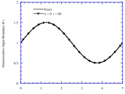
0 0.5 1 1.5 2 0 1 2 3 4 5 Exact = 0 r = 60 D im en si o n le ss In p u t B o u n d ar y ( ) Dimensionless Temporal-Coordinate ()

Figure 3: The inverse solution of sinusoidal-polynomial function when

0   and r60 0 0.5 1 1.5 2 0 1 2 3 4 5 Exact = 0.01 r = 65 = 0.02 r = 65 = 0.02 r = 70 D im en si o n le ss In p u t B o u n d ar y ( ) Dimensionless Temporal-Coordinate ()

Figure4: The inverse solution of sinusoidal-polynomial function when

01 . 0   r 65, 0.02 r 65, and 0.02 r 70 0 0.5 1 1.5 2 0 1 2 3 4 5 Exact = 0 r = 60 D im en si o n le ss In p u t B o u n d ar y ( ) Dimensionless Temporal-Coordinate ()

Figure 5: The inverse solution of

stepwise function when 0 and

60  r 0 0.5 1 1.5 2 0 1 2 3 4 5 Exact = 0.01 r = 65 = 0.02 r = 65 = 0.02 r = 70 D im e n si o n le ss In p u t B o u n d a ry ( ) Dimensionless Temporal-Coordinate ()

Figure6: The inverse solution of

stepwise function when 0.01

65  r , 0.02 r65, and 02 . 0   r 70 0 0.5 1 1.5 2 0 1 2 3 4 5 Exact = 0 r = 60 D im e n si o n le ss In p u t B o u n d a ry ( ) Dimensionless Temporal-Coordinate ()

Figure 7: The inverse solution of

triangular function when 0 and

60  r 0 0.5 1 1.5 2 0 1 2 3 4 5 Exact = 0.01 r = 65 = 0.02 r = 65 = 0.02 r = 70 D im en si o n le ss In p u t B o u n d ar y ( ) Dimensionless Temporal-Coordinate ()

Figure 8: The inverse solution of

triangular function when 0.01

65  r , 0.02 r65, and 02 . 0   r 70 研究中顯示，不連續之直接解0.45 與  ，如圖 2 所示。計畫中以1 sinusoidal-polynomial 函數、 stepwise 函數與 triangular 函數，當為估算之邊 界，圖 3-8 分別顯示上述三種不同邊界

估算之結果。結果顯示，對不同之邊 界估算，本研究法均可有效解決此類 多維非傅利葉逆熱傳導問題。 計畫結果自評 本研究所討論之方法可有效運用 於多維非傅利葉逆運算問題。計畫中 先行推導直接 解問題 ，再運用修正 Newton-Raphson 解決逆問題。結果顯 示研究中所用方法，可有效解決多維 非傅利葉逆運算問題。 參考文獻

1. Whey-Bin Lor and Hsin-Sen Chu, “Effect of interface thermal resistance on heat transfer in a composite medium using the thermal wave model,”International Journal of Heat and Mass Transfer, Vol. 43, pp.653-663, 2000.

2. Paul J. Antaki, :Importance of NonFourier Heat Conduction in Solid-Phase Reactions, “Combustion and Flame, Vol. 112, pp. 329-341, 1998.

3. Terry Sanderson, Charles Ume and Jacek Jarzynski, “Hyperbolic heat equations in laser generated ultrasound models, “Ultrasonics, Vol. 33, No. 6,pp.415-421, 1995.

4. L. H. Liu, H. P. Tan, and T. W. Tong, “Non-Fourier effects on transient temperature response in semitransparent medium caused by laser pulse,”International Journal of Heat and Mass Transfer, Vol. 44, pp.3335-3344, 2001. 5. Andrew M. Mullis, “Rapid solidification and a finite velocity for the propagation of heat,” Material Science and Engineering, A226-228, pp28-32, 1997.

6. Andrew M. Mullis, “Rapid solidification within the framework of a hyperbolic conduction model,”International Journal of Heat and Mass Transfer, Vol. 40, No 17, pp.4085-4094, 1997. 7. Ranjit Kumar Sahoo and Wilfried Roetzel, “Hyperbolic axial dispersion model for heat exchangers,”International Journal of Heat and Mass Transfer, Vol. 45, pp.1261-1270, 2002. 8. Wilfried Roetzel and Sarit K. Das,”Hyperbolic axial dispersion model: concept and its application to a plate heat exchanger,” International Journal of Heat and Mass Transfer, Vol. 38, No. 16, pp.3065-3076, 1995.

9. Wilfried Roetzel and Chakkrit Na Ranong, Consideration of maldistributation in heat exchangers using the hyperbolic dispersion model, Chemical Engineering and Processing, Vol 38, pp675-681, 1999.

10. Jae-Yuh Lin, “The non-Fourier effect on the fin performance under periodic thermal conditions,”Applied Mathematical Modelling,

Vol. 22,pp.629-640, 1998.

11. Bishri Abdel-Hamid, “Modelling non-Fourier heat conduction with periodic thermal oscillation using the finite integral transform,” Applied Mathematical Modelling, vol. 23, pp899-914, 1999.

12. D. W. Tang and N. Araki, “Non-Fourier heat conduction in a finite medium under periodic surface thermal disturbance,” International Journal of Heat and Mass Transform, Vol. 39, No. 18, pp.1585-1590 13. Zhi-Ming Tan and Wen-Jei Yang,”Propagation of thermal waves in transient heat conduction in a thin film,”Journal of The Franklin Institute, Vol. 336B, pp185-197, 1999. 14. Zhi-Ming Tan and Wen-Jei Yang,”Heat transfer during asymmetrical collision of thermal waves in a this film,”International Journal of Heat and Mass Transfer, Vol. 40, No. 17, pp.39999-4006, 1997.

15. H. Q. Yang, Solution of two-dimensional hyperbolic heat conduction by high-resolution numerical method, Numerical Heat Transfer A21,333-349, 1992.

16. H. T. Chen and J. Y. Lin, Analysis of two-dimensional hyperbolic heat conduction problems, International Journal Heat and Mass Transfer, vol. 37, 1,153-164, 1993,1994.

17. Weber C. Analysis and solution of the ill-posed inverse heat conduction problem, International heat and Mass Transfer, 1981:24:1783-91

18. Nehad Al-Khalidy, On the solution of parabolic and hyperbolic inverse heat conduction problems, International Journal of Heat and Mass Transfer, 41, pp3731-3740, 1998.

19. Nehad Al-Khalidy, Analysis of boundary inverse heat conduction problems using space marching with Savitzky-Gollay digital filter, International Communication of Heat and Mass Transfer, 26, 2, pp.199-208, 1999.

20. H. T. Chen, S. Y. Peng, and L. C. Fang, Numerical method for hyperbolic inverse heat conduction problems, International Communication of Heat and Mass Transfer, 28, 6, pp847-856, 2001.

21. Yang, C. Y., 2005 “Direct and Inverse Solutions of the Hyperbolic Heat Conduction Problems," AIAA Journal of Thermophysics and

出席國際學術會議心得報告

計畫編號

NSC94-2212-E-151-019-計畫名稱 二維非複利葉熱傳導問題之正解與逆解之理論與實驗研究

出國人員姓名

服務機關及職稱 國立高雄應用科技大學模具系 教授楊慶煜

會議時間地點 Sep.4-8,2006 Toyama Japan

會議名稱 ISTP-17

發表論文題目 Inverse Estimation of Two-dimensional Boundary Conditions in

Bio-Heat Conduction Problems

一、 參加會議經過

本次會議主要探討熱流與質傳現象之發展，會議於 2006 年 9 月 4 日至 8 日舉

辦。主要內容包含了實驗與計算流體力學、航太工程、電子熱傳、燃燒、生

物熱傳、熱交換器、能源系統等十餘項主題並辦有四場 Keynote lectures。

共有數百餘篇論文參予此次會議。本人發表之論文亦於會議中以口頭形式報

告論文，也承蒙許多學者提問與討論，獲益匪淺。

二、 與會心得

期望來年能持續參與 ISTP 相關會議，並邀請知名學者到國內講學與研究。本

人所屬單位亦有意願爭取主辦本項研討會，增加與國外學者交流之機會。

參、攜回資料

會議手冊