並聯矩陣整合型發電風車動力效率數值分析

(1)

國立交通大學

機械工程學系

碩士論文

並聯矩陣整合型發電風車動力效率

數值分析

A Numerical Analysis of Power Efficiency of Wind

Rotor System in Parallel Matrix

研究生：馮嘉軒

指導教授：陳俊勳教授

(2)

並聯矩陣整合型發電風車動力效率數值分析

A Numerical Analysis of Power Efficiency of Wind Rotor System in Parallel Matrix 研究生：馮嘉軒 Student：Jia-Shiuan Feng 指導教授：陳俊勳 Advisor：Chiun-Hsun Chen 國立交通大學機械工程學系碩士論文 A Thesis

Submitted to Department of Mechanical Engineering College of Engineering

National Chiao Tung University In Partial Fulfiillment of the Requirements

For the Degree of Master of Science In Mechanical Engineering

June 2011

Hsinchu, Taiwan, Republic of China

(3)

i

A Numerical Analysis of Power Efficiency of Wind Rotor System in Parallel Matrix 並聯矩陣整合型發電風車動力效率數值分析 學生 : 馮嘉軒指導教授 : 陳俊勳國立交通大學機械工程學系

摘要

本研究使用流體力學套裝軟體 Fluent 分析二葉式 Savonius 風車周圍的流場與效能，研究主題分為單一風車與並聯矩陣系統，改變參數為風速、周速比及相位角差，此外探討風向對並聯矩陣系統的影響，最後討論兩個主題的差異，並與其他文獻之提升效能方法進行比較。從模擬結果可得知，單一風車在同一周速比的情況下，功率係數（cp）會隨風速提升而略微提高，另外比較單一風車在大氣與風洞中的情境後發現，由於風洞中邊界的影響，使得風車在大氣中的效能會低於在風洞中的情境。二維模擬結果顯示，在並聯矩陣系統中，相位角差 90°可得到最好的 cp，為單一風車情況下的 2.05 倍。並聯矩陣系統的效能提升主要歸因於風車間的正向干擾情形，而流場的波動現象在此效應中扮演主要角色，但此種正向干擾效應受風向改變的影響極大。當風向改變 45°時，其效能會趨近於甚至低於單一風車情況下的效能。在三維模擬中，並聯矩陣系統的最大效能會達到單一風車的 1.45 倍，另外比較二維與三維 cp 的差異，在單一風車條件下其比值為 1.28，而在並聯矩陣系統中為 1.83。關鍵字：Savonius 風車、並聯矩陣系統、功率係數

(4)

ii

A Numerical Analysis of Power Efficiency of Wind Rotor System in Parallel Matrix

Student: Jia-Shiuan Feng Advisor: Prof. Chiun-Hsun Chen Department of Mechanical Engineering

National Chiao Tung University

ABSTRACT

This study employs a computational fluid dynamics (CFD) software, Fluent, to analyze the flow fields around two-bladed Savonius wind rotors and their corresponding performances. It is divided into two topics: one is a study of a single Savonius wind rotor, and the other is of a parallel matrix system. Both are carried out by the related parametric studies. The parameters for the single wind rotor are wind velocity and tip speed ratio. The ones for the parallel matrix system are wind velocity, tip speed ratio, phase angle difference and wind direction change. Then, comparison between the two systems is discussed. Besides, comparisons with other studies are also given.

The simulation results show that the cp (power coefficient) of a

single wind rotor slightly increases with wind speeds at the same tip speed ratio, and the performance of the one in atmosphere is lower than that inside the wind tunnel due to the influence of walls. In the 2-D simulation results of parallel matrix system, phase angle difference 90° can obtain the best cp that is 2.05 times of that by a single wind rotor. The

higher performance of parallel matrix system is resulted from the positive interaction between these Savonius wind rotors, and the flow fluctuation

(5)

iii

plays the major role in contributing to this effect, but this effect is strongly influenced by the change of wind direction. When wind direction is 45°, the cp of the parallel matrix system becomes almost the same or

even lower than that of a single one. The maximal cp in the parallel matrix

system by 3-D simulation is about 1.45 times of that by a single Savonius wind rotor. The ratio of 2-D cp to 3-D one is 1.28 in the single Savonius

wind rotor condition and 1.83 in the parallel matrix system.

Keywords: Savonius wind rotor; parallel matrix system; cp (power

(6)

iv

ACKNOWLEDGEMENTS

首先必須感謝我的指導教授陳俊勳教授，總是耐心地糾正我的錯誤並給予指導，使我在這兩年內學習到許多處理事情與解決問題的能力。感謝曾錦鍊學長給了我這個題目並也給予許多指導。感謝老朋友伯華教導我許多風車模擬的技巧，淑敏在指導我的英文上有莫大的幫助，還有崔燕勇師門的林子翔同學也在模擬上給予我許多建議。另外也感謝國科會計畫的經費支持。再來是感謝這兩年陪我一起度過的實驗室的諸位。云婷開心的笑聲是我每天的動力來源，當我遇到許多煩惱時妳也總是靜靜的聆聽並給予我建議與鼓勵。聖容是實驗室最厲害的開心果，沒有妳的話這兩年生活一定會失色不少。世庸是最常與我相處在一起的人，不管在瑣事還是正事上都給我許多幫助。與你們三個住在一起的這一年，一定是我這一生中非常重要的回憶。還有總是睡不飽的黃鈞，也是我一同前進與成長的好夥伴。感謝學長榮貴、瑭原、宗翰給予過我許多幫助，家維學長與彥成學長在模擬上也給了我許多建議，學弟凌宇、詠翔、鉦鈞與天洋則總是為我帶來歡笑，衷心希望你們接下來一年也能每天都開懷大笑。感謝所有曾經給過我鼓勵的朋友們，雖然可能一時無法把名字都一一點出來，但你們曾經給予過我的，我都不會忘記。最後，必須鄭

(7)

v 重感謝我的父母，雖然我很常感到彷徨失措，但你們總相信自己的兒子一定是最好的，一定不會問題的，也永遠以笑容迎接我回家，這才是我在遇到挫折時還能繼續前進的最大動力。還有我親愛的哥哥與堂姐，你們的鼓勵也是這兩年不容忽視的一環。也許我還不成熟，對於未來也依然感到茫然，只能持續摸索，但我知道在這兩年得到的許多珍貴的經驗與回憶，那是什麼都無法換走的。

(8)

vi

LIST OF TABLE

Table 3.1 Geometry Information ... 21 Table 3.2 Dimensions of Domains ... 22 Table 3.3 Grid Numbers of all the Domains ... 40 Table 4.1 Parameters for a single Savonius wind rotor inside the wind tunnel (Reference case) ... 48 Table 4.2 Parameters for a single Savonius wind rotor in atmosphere .... 51 Table 4.3 Parameters for three-rotor in atmosphere ... 53 Table 4.4 Comparisons of the maximums of cp between a single rotor and

three-rotor in 2-D simulations ... 55 Table 4.5 Comparisons of the maximum cps between a single rotor and

three-rotor with phase angle difference 90° in 3-D simulation ... 58 Table 4.6 The maximums of average power output of a Savonius wind rotor in the two systems ... 59

(12)

x

LIST OF FIGURES

Fig. 1.1 Evolution of global population and global carbon dioxide

emissions since 1900 ... 9

Fig. 1.2 Life cycle CO2 emission factors for different types of power generation systems [16] ... 9

Fig. 1.3 Wind turbine configurations ... 10

Fig. 1.4 Schematic of a two-bladed Savonius wind rotor [4] ... 10

Fig. 1.5 VAWT with windshield [6] ... 11

Fig. 1.6 The scope of this study ... 11

Fig. 2.1 Idealized fluid model for a wind rotor [17] ... 19

Fig. 2.2 Typical power coefficients of different wind rotor types over tip-speed ratio [17] ... 19

Fig. 2.3 Flow conditions and aerodynamic forces with a drag device [18] ... 20

Fig. 2.4 Aerodynamic forces acting on an airfoil exposed to an air stream [18] ... 20

Fig. 3.1 The domain for one single Savonius wind rotor inside the wind tunnel (Reference) ... 41

Fig. 3.2 The domain for one single Savonius wind rotor in atmosphere . 41 Fig. 3.3 The domain for three Savonius wind rotors in atmosphere ... 41

Fig. 3.4 The domain for three Savonius wind rotors in atmosphere with different wind direction (θ=0°, ±15°, ±30°, ±45°) ... 42

Fig. 3.5 Overview of the Segregated Solution Method ... 42

Fig. 3.6 Control Volume Used to Illustrate Discretization of a Scalar Transport Equation ... 43

(13)

xi

Fig. 3.7 Zones Created by Non-Periodic Interface Intersection ... 43

Fig. 3.8 Two-Dimensional Grid Interface ... 44

Fig. 3.9 User Interface of Gambit ... 44

Fig. 3.10 Grid-independence tests ... 46

Fig. 4.1 The experimental results of a single Savonius wind rotor inside the wind tunnel (Reference case) [4] ... 62

Fig. 4.2 The defined angle α of rotating wind rotor relative to the initial angle ... 62

Fig 4.3 Torque curve of one single Savonius wind rotor inside the wind tunnel with wind speed 7 m/s and tip-speed ratio 0.9 in a rotation 63 Fig. 4.4 Static pressure field around one single Savonius wind rotor inside the wind tunnel in 2-D simulation ... 64

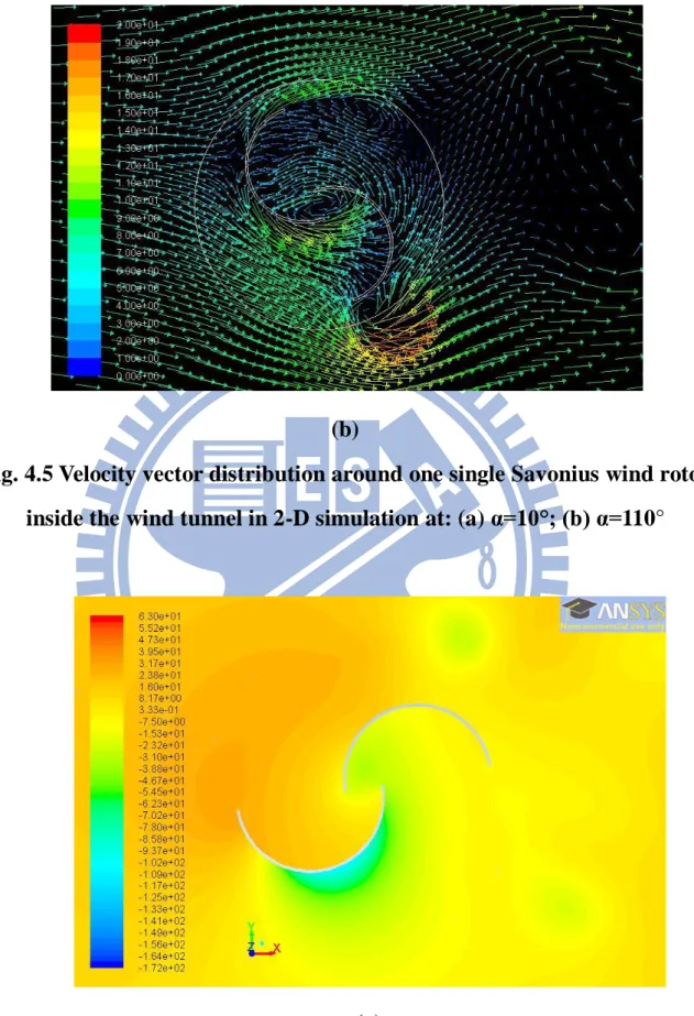
Fig. 4.5 Velocity vector distribution around one single Savonius wind rotor inside the wind tunnel in 2-D simulation... 65

Fig. 4.6 Static pressure field around one single Savonius wind rotor inside the wind tunnel in 3-D simulation at z = 1m ... 66

Fig. 4.7 Velocity vectors distribution around one single Savonius wind rotor inside the wind tunnel in 3-D simulation at z = 1m ... 67

Fig. 4.8 Velocity vector distribution in 3-D simulation at y = 0 ... 68

Fig. 4.9 A single Savonius wind rotor inside the wind tunnel comparing with experimental data ... 69

Fig. 4.10 The performance of a single Savonius rotor inside the wind tunnel ... 69

Fig. 4.11 Velocity vector distribution around one single Savonius wind rotor inside the wind tunnel at z=1m and α=110° ... 70 Fig 4.12 Torque curve of one single Savonius wind rotor in atmosphere

(14)

xii

with wind speed 7 m/s and tip-speed ratio 0.9 in a rotation ... 71 Fig. 4.13 Static pressure field around one single Savonius wind rotor in atmosphere in 2-D simulation... 72 Fig. 4.14 Velocity vector distribution around one single Savonius wind rotor in atmosphere in 2-D simulation ... 73 Fig. 4.15 Static pressure field around one single Savonius wind rotor in atmosphere in 3-D simulation at z=1m ... 74 Fig. 4.16 Velocity vector distribution around one single Savonius wind rotor in atmosphere in 3-D simulation at z=1m ... 75 Fig. 4.17 The performance of a single Savonius wind rotor in atmosphere

... 75 Fig. 4.18 Streamlines around one single Savonius wind rotor ... 76 Fig. 4.19 Streamlines around one single Savonius wind rotor ... 77 Fig. 4.20 Performance comparisons between one single Savonius wind rotor inside the wind tunnel and one in atmosphere ... 78 Fig. 4.21 Torque curves of the three Savonius wind rotor with phase angle difference 90° in wind speed 7 m/s at tip-speed ratio 0.9 ... 79 Fig. 4.22 Static pressure field around three Savonius wind rotors with phase angle difference 90°... 80 Fig. 4.23 Velocity vector distribution around three Savonius wind rotors with phase angle difference 90° ... 81 Fig. 4.24 Performances of three-rotor with different phase angle differences in 2-D simulation ... 82 Fig. 4.25 Streamlines around three Savonius wind rotors with phase angle difference 90° ... 83 Fig. 4.26 Three-rotor with phase angle difference 90° in different wind

(15)

xiii

directions... 83 Fig. 4.27 Velocity vector distribution around the three Savonius wind rotors with a change of wind direction θ = -45° ... 84 Fig. 4.28 Static pressure field around three Savonius wind rotors in 3-D simulation at z=1m ... 85 Fig. 4.29 Velocity vector distribution around three Savonius wind rotors in 3-D simulation at z=1m ... 86 Fig. 4.30 Performances of three-rotor with phase angle difference 90° in 3-D simulation ... 87 Fig. 4.31 Performance comparisons between 2-D and 3-D simulations .. 88 Fig. 4.32 Velocity vector distribution in 3-D simulations at x=0 ... 89

(16)

1

CHAPTER 1 INTRODUCTION

1.1 Motivation

The world population is increasing at a fast rate, and the growth rate especially is quite high in developing countries. According to the calculation and projection of world population by the United Nations, there are 6.4 billion people in 2004, and the population will grow up to 8.5 billion in 2025 and 10 billion in 2050. As expected, the demands for energy and food are increasing simultaneously.

In 2008, total worldwide energy consumption was 474 exajoules (474×1018 J) with 80 to 90 percent from the combustion of fossil fuels. Dependence on fossil fuels may cause serious problems including not only the energy shortage crisis but also the rapid change of global climate due to carbon dioxide emissions. The dramatic rise in carbon dioxide emissions over the 20th and early 21st centuries (see Fig. 1.1) is because of the anthropogenic burning of fossil fuels primarily. Therefore, to replace fossil fuels with renewable energy causing no environmental impacts becomes an important issue. Fig. 1.2 shows that renewable energy, such as the wind power or solar energy, has very low carbon dioxide emissions during production. Although nuclear energy emits no carbon dioxide during power generation either, but the impact of nuclear waste would cause more severe environmental problems than that of carbon dioxide emissions. Hence, researches of renewable energy are extremely of importance, and wind power plays an important role in this field.

Wind power is the conversion of wind energy into a useful form of energy by functioning wind turbines. They are classified into horizontal axis wind

(17)

2

turbine (HAWT) and vertical axis wind turbine (VAWT) according to their appearances as shown in Fig. 1.3. The rotational axis of HAWTs is horizontal to the ground, and that of VAWTs is vertical. After a long period of development, almost all of the wind power generation systems adopt HAWTs because of their higher cp (Power Coefficient) comparing to the one of VAWTs. Generally

speaking, the cp of HAWTs is ranged from 0.30 to 0.45, and that of VAWTs is

about 0.15 to 0.30. However, there are some problems in using HAWTs. First, the high tip speed ratio of HAWTs causes low-frequency noise. Second, the distance between HAWTs should be sufficient to avoid interferences of wind fields. Third, sometimes HAWTs take a long time to be oriented in the wind direction. Last but not least, it might be a huge cost to install a HAWT for its land preparations, installation, maintenance, and repair. Therefore, feasibilities of VAWTs, which have lower costs and simple structures but with lower cp

should be taken into account with some improvements.

Although the cp of VAWTs is lower than the one of HAWTs, there are ways

to improve their performance. This research proposes an idea to achieve this purpose. Such idea is to put a plurality of VAWTs connecting in parallel with a fixed distance between them and they rotate with a specific phase angle difference. In this way, the performance would be improved by utilizing wind fields effectively. By adopting this idea, the present work is interesting in investigating the performance differences between a single general Savonius wind rotor (see Fig. 1.4) and a plurality of those installed in parallel by using Computational Fluid Dynamics (CFD) technique.

(18)

3

1.2 Literature Review

Shigetomi et al. [1] studied the interactive flow field around two Savonius wind rotors by experimental investigation using particle image velocimetry. They found that there exist power-improvement interactions between two rotating Savonius rotors in appropriate arrangements. The interactions are caused by the Magnus effect to provide the additional rotation of the downstream rotor and the periodic coupling of local flow between two wind rotors. However, the interactions of two wind rotors are sensitive to the direction of wind losing one of the advantages of VAWTs.

Antheaume et al. [2] applied a CFD software, Fluent, to investigate the performances of vertical-axis Darrieus wind rotors in different working fluids by using k-ε turbulent model under steady-state condition. They also discussed the average efficiency of several wind rotors connected in parallel. The results showed that increasing the number of wind rotors or decreasing the distance between wind rotors can make the efficiency higher due to the velocity streamlines straightening effect by the configuration. In addition, the performances working in water are much higher than those in air.

Fujisawa [3] studied the performances of two-bladed Savonius wind rotors with different overlap ratios ranged from 0 to 0.5 by experimental investigations. The results showed that the performance of a Savonius wind rotor reaches a maximum at overlap ratio 0.15 because the advancing blade is strengthened by the flow through the overlap. When the overlap ratio becomes larger, the recirculation zone grows causing a deterioration of the performance.

Blackwell et al. [4] investigated the performances of fifteen configurations of Savonius wind rotors by testing in a low speed wind tunnel. What they

(19)

4

investigated included parameters, such as number of blades, wind velocity, wind rotor height, and blade overlap ratio. The results showed that first of all, the two-bladed configurations have better performance than the three-bladed ones, except starting torque. Second, the performance increases with aspect ratio slightly. Last, the optimum overlap ratio is 0.1 to 0.15.

Pope et al. [5] applied Fluent to investigate the performances of one VAWT and compared the predictions with experimental data. By the reason that a free spinning turbine cannot be fully simulated, they used constant rotational speeds of the VAWT in simulations and changed the specification of parameters to reveal freely moving turbine blades in experiments. They indicated that determining the performance at constant rotational speed is valuable since any power generation connected to the electricity grid needs to operate at constant speed.

Howell et al. [6] applied Fluent to investigate the performances of one VAWT in 2-D and 3-D simulations and compared the predictions with experimental data. The turbulence model used was RNG k-ε model, by which the applicability in flow fields involves large flow separations. The error bars on experimental data were fixed at ±20% of measured values. The results showed that the performances predicted by 2-D simulations are apparently higher than those by 3-D simulations and experimental data due to the effect of the over tip vortices.

Hu and Tong [7] used Fluent to analyze the performances in VAWT with windshield for decreasing the counter torque as shown in Fig. 1.5. They used k-ε RNG turbulent model and SIMPLE algorithm in 2-D simulations. The results showed that about 15° of inclination angle between the bottom of windshield and x-axis gives the highest value of torque.

(20)

5

Kamoji et al. [8] compared the performance differences between conventional Savonius wind rotors with and without central shaft between the end plates in an open jet wind tunnel. Investigation was undertaken to study the effects of overlap ratio, blade arc angle, aspect ratio and Reynolds number. The results showed that the performance of the Savonius wind rotor without central shaft is higher than that with central shaft.

Altan et al. [9] introduced a curtaining arrangement to improve the performance and increase the efficiency of a tow-bladed Savonius wind rotor without changing its basic structure. They placed two wind-deflecting plates in front of the wind rotor to prevent the negative torque opposite the wind rotor rotation. The experimental results showed that cp is increased to about 38% with

the optimum curtain arrangement and is much higher than 16% obtained without curtain.

Mohamed et al. [10] used a CFD software to investigate the performances of two-bladed and three-bladed Savonius wind rotors with and without putting an obstacle to prevent the influence of wind on the returning blade. They concluded that an appropriate arrangement of the obstacle can increases cp by

27.3% for two-bladed Savonius wind rotors and 27.5% for three-bladed ones. Therefore, the overall effect of the obstacle is extremely positive for both designs. Furthermore, the two-bladed wind rotors are better than three-bladed configurations by considering the resultant cp and the cost and complexity of the

wind rotor.

Saha et al. [11] used a wind tunnel to test and investigate the performances by different number of blades and stages, different geometries of blade and inserting valves on the concave side of blade or not. The results were as follows. First, with an increases of the number of blades, the performance of wind rotor

(21)

6

decreases. Second, twisted geometry blade profile has a better performance than the semicircular blade geometry. Third, the cp of a two-stage Savonius wind

rotor is higher than those of single-stage and three-stage wind rotors. Last, the valve-aided Savonius wind rotor with three blades shows a better performance than the conventional wind rotor.

Zhao et al. [12] applied computational fluid dynamics software to investigate the performance of new helical Savonius wind rotors. They analyzed the differences of the wind rotors with different aspects ratio, number of blades, overlap distance and helical angle. The results showed that three-blade helical wind rotor has lower cp compared with two-bladed helical wind rotor. And the

best overlap ratio, aspect ratio, and helical angle are 0.3, 6.0 and 180°, respectively.

Gupta et al. [13] studied the performances of a Savonius wind rotor and a Savonius-Darrieus machine with overlap variation by experimental investigations. For the Savonius-Darrieus machine, there was a two-bladed Savonius wind rotor in the upper part and a Darrieus machine in the lower side. The result showed that cp with 20% overlap is higher than 16.2% without

overlap. They also concluded that the improvement of cp can be achieved for the

Savonius-Darrieus wind machine compared with the general Savonius rotor. Irabu and Roy [14] introduced a guide-box tunnel to improve the cp of

Savonius wind rotors and prevent the damage by strong wind disaster. The guide-box tunnel was like a rectangular box as wind passage and the test wind rotor was included. It was able to adjust the inlet mass flow rate by its variable area ratio between the inlet and outlet. The experimental results showed that the maximum cp of the two-bladed wind rotor using the guide-box tunnel is about

(22)

7

a three-bladed wind rotor. Besides, the two-bladed wind rotor is better than the three-bladed in converting wind power through guide-box tunnel effectively, except the starting rotation.

Chinchilla et al. [15] studied the need for further researches and developments on improved airfoil or blade characteristics on straight bladed VAWT. They indicated that the asymmetric airfoils would enable VAWTs to self start and could be utilized in the regions of low or turbulent air.

Chang et al. [16] analyzed wind characteristics and wind turbine characteristics in Taiwan by mathematical formulations using the measured data of hourly mean wind speed at 25 weather stations from 1961 to 1999. They indicated that in the west coast, Hengchun Peninsula and some small surrounding islands, there are outstanding wind sources being suitable for wind power generation.

1.3 Scope of Present Study

This study employs a computational fluid dynamics (CFD) software, Fluent, to analyze the flow fields around two-bladed Savonius wind rotors and their corresponding performances. The scope of this study is illustrated in Fig. 1.6. First, a reference case is established, and the comparison between simulation results and experimental data is given to ensure the capability of the applied model. Then this research is divided into two topics: one is a study of a single Savonius wind rotor, and the other is of a parallel matrix system. Both the two topics are carried out by the corresponding parametric studies. The parameters for the single wind rotor are wind velocity and tip speed ratio, and for the parallel matrix system are wind velocity, tip speed ratio and phase angle

(23)

8

difference. After that, the influence of wind direction change on the parallel system is also studied. Then, comparisons between the two systems are discussed. Besides, comparisons with other researches, such as improvements by adding windshields or twisted rotor systems, are also given.

(24)

9

Fig. 1.1 Evolution of global population and global carbon dioxide emissions since 1900

http://www.worldclimatereport.com/index.php/2008/01/30/what-the-future-hold s-in-store/

Fig. 1.2 Life cycle CO2 emission factors for different types of power generation systems [16]

(25)

10

Fig. 1.3 Wind turbine configurations

http://colonizeantarctica.blogspot.com/

(26)

11

Fig. 1.5 VAWT with windshield [6]

Two-bladed Savonius Rotors Reference case Single wind rotor Parallel wind rotors system Wind velocity Tip speed ratio Wind velocity Tip speed ratio Wind direction Phase angle difference

(27)

12

CHAPTER 2 FUNDAMENTALS OF WIND ENERGY

2.1 Brief History of Wind Energy

The first wind machine was known as appearing about 2200 years ago in Persia for grinding grains. Then the Romans used the same way for the same purpose around 250 A.D. By the fourteenth century, the Dutch employed windmills to drain water in the low-lying areas of the Rhine River delta.

The first use of windmill for producing electricity was in 1888. And the first such windmill was built and used by Charles Brush in Ohio, U.S.A. Ten years later, about 72 wind turbines were being used to produce electricity in the range of about 5 to 25kW.

In the twentieth century, wind turbines were used around the world. There existed many small electricity generating sites in Denmark, and wind power was a large part of them. In Australia, wind turbines were used to power remote post offices. In America, rural farms had used wind power originally. Eventually, this generated electricity was connected to grid later. By 1930, more than six million wind turbines had been manufactured in American and it was the first time that the utilization of wind energy was based on an industrially mass-produced. The first megawatt wind turbine was built in USA in 1941. In the 1970s and 1980s, the U.S. Government promoted the technology through NASA and researched many of the designs that still use today.

In the end of 2002, there was roughly 32GW of power supplied from wind energy in the world. Europe has been the leader in wind power utilization, contributing 76% of the total. In 2006, roughly 65GW of rated power were installed in wind farms worldwide, of which more than 47GW located in Europe,

(28)

13

and more than 11GW in the United States.

2.2 Basics of Wind Energy Conversion

2.2.1 Power Conversion and Power Coefficient

From the expression for kinetic energy in flowing air, the power contained in the wind passing an area A with the wind velocity v1 is:

P_W = ρ

2Av1

3

(2-1) where ρ is air density, depending on air pressure and moisture. For practical calculations it may be assumed ρ ≈ 1.225kg/m3

. The air streams in axial direction through the wind turbine, of which A is the swept area. The useful mechanical power obtained is expre2ssed by means of the power coefficient cp:

P = c_p ρ

2Av1

3

(2-2) The wind velocity, whose value ahead of the turbine plane is v1, suffers

retardation due to the power conversion to a speed v3 far behind the wind turbine,

as shown in Fig. 2.1. Simplified theory claims that in the plane of the moving blades the velocity is of average value v2 = (v1 + v3)/2. On this basis, Betz has

shown by a simple calculation that the maximum useful power can be obtained for v3/v1 = 1/3 in 1920; where the power coefficient cp = 16/27 ≈ 0.593. In reality,

wind turbine displays the maximum values cp, max = 0.4 ~ 0.5 due to losses, such

as profile loss, tip loss and loss due to wake rotation. In order to determine the mechanical power available for the load machine, such as electrical generator or pump, Eq. (2-2) has to be multiplied with an efficiency of the drive train, taking losses in bearings, couplings and gear boxes into account.

(29)

14

as a ratio of the circumferential velocity of blade tips to the wind speed: λ _{= u v} =₁ D₂ ∙ ω

v₁

(2-3) where D is the outer turbine diameter and ω the angular wind rotor speed.

Considering that in the rotating mechanical system, the power is the product of torque T and angular speed ω (P = T · ω), then cp becomes

c_p = P PW = T⋅ω 1 2ρAv13 (2-4)

Fig. 2.2 shows typical characteristics cp (λ) for different types of wind

rotors. Besides the constant maximum value according to Betz, the figure indicates a revised curve cp by Schmitz, who takes the downstream deviation

from axial air flow direction into account. The difference is notable in the region of lower tip speed ratios.

2.2.2 Wind Energy Converters Using Aerodynamic Drag or Lift

The momentum theory by Betz indicates the physically based, ideal limit value for the extraction of mechanical power from free-stream airflow without considering the design of the energy converter. However, the power which can be achieved under real conditions cannot be independent of the characteristics of the energy converter. The first fundamental difference which considerably influences the actual power depends on which aerodynamic forces are utilized for producing mechanical power. All bodies exposed to an airflow experience aerodynamic forces, which are defined as aerodynamic drag in the flow direction, and as aerodynamic lift perpendicular to the flow direction. The real power coefficients obtained are greatly dependent on whether aerodynamic drag or aerodynamic lift is used.

(30)

15

2.2.2.1 Drag Devices

The simplest type of wind energy conversion can be achieved by means of pure drag surfaces as shown in Fig. 2.3. The air impinges on the surface A with wind velocity v, and then the drag D can be calculated from the air density ρ, the surface area A, the wind velocity v, and the aerodynamic drag coefficient cD as

D = c_D 1

2ρAvr

2 _{= c}

D1₂ρA v − u 2 (2-5)

The relative velocity, vr = v – u, which effectively impinges on the drag area, is

determined by wind velocity v and blade rotating speed u = ωRM, in which RM is

the mean radius. Then the resultant power is P = D ⋅ u = 1

2ρAv

3_c

D 1 −u_v 2 u_v = 1₂ρAv3cp (2-6)

Analog to the approach described in Chapter 2.2.1, it can be shown that cp

reaches a maximum value with a velocity ratio of u/v = 1/3. The maximum value of cp is then

c_p,max = 4

27cD

(2-8) It is taken into account that the aerodynamic drag coefficient CD of a

concave surface curved against the wind direction can hardly exceed a value of 1.3. Thus, the maximum power coefficient cp, max of a general drag-type wind

rotor becomes about 0.2, only one third of Betz’s ideal cp value of 0.593.

2.2.2.2 Lift Devices

Utilization of aerodynamic lift on wind rotor blade can achieve much higher power coefficients. The lift blade design employs the same principle that enables airplanes to fly. As shown in Fig. 2.4, when air flows over the blade, a pressure gradient is created between the upper and lower blade surfaces. The pressure at the lower surface is greater and thus acts to lift the blade. The lift

(31)

16

occurred on a body by wind can be calculated from the air density ρ, acting area A, wind speed v, and aerodynamic lift coefficient cL as

L = c_L1

2ρAv

2

(2-9) When blades are attached to the central axis of a wind rotor, the lift is translated into rotational motion. All modern wind rotor types are designed for utilizing this effect, and the best type suited for this purpose is with a horizontal rotational axis. The aerodynamic force created is divided into a component in the direction of free-stream velocity, the drag D, and a component perpendicular to the free-stream velocity, the lift L. The lift force L can be further divided into a component Ltorque in the plane of rotation of the wind rotor, and a component

Lthrust perpendicular to the plane of rotation. Ltorque constitutes the driving torque

of the wind rotor.

Modern airfoils, developed for aircraft wings and which are also applied in wind rotors, have an extremely favorable lift-to-drag ratio. It could show qualitatively how much more effective the utilization of aerodynamic lift as a driving force must be. However, it is no longer possible to calculate the power coefficients of lift-type wind rotors quantitatively with the aid of elementary physical relationships alone.

2.3 Vertical and Horizontal Axis Wind Rotors

Wind rotors are approximately classified into two general types by their orientations: horizontal-axis type and vertical-axis type. A horizontal-axis wind rotor has its blades rotating on an axis parallel to the ground and a vertical-axis one has that rotating on an axis perpendicular to the ground. There are a number of designs for both, and each type has certain advantages and disadvantages.

(32)

17

However, the number of vertical-axis wind rotor for commercial uses is much less than that of horizontal-axis wind rotor.

2.3.1 Wind Rotors with a Vertical Axis of Rotation

The oldest design of wind rotors is with a vertical axis of rotation. At the beginning, vertical-axis wind rotors could only be built for using aerodynamic drag. It was only recently that engineers succeeded in developing vertical-axis designs which could also utilize aerodynamic lift effectively. Darrieus proposed such design which has been considered as a promising concept for modern wind turbines in 1925. The Darrieus wind rotor resembles a gigantic eggbeater and the geometric shape of the wind rotors blades is complicated that is difficult to manufacture. Furthermore, there is a variation of the Darrieus wind rotor which is called H-rotor. Instead of curved wind rotor blades, straight blades connected to the wind rotor shaft by struts are used.

Savonius wind rotor, which is investigated in this research, is also one type of vertical-axis wind rotors. The wind rotor was invented by a Finnish engineer, Savonius in 1922. Savonius wind rotor is one of the simplest wind rotors to manufacture. Because it is drag-type devices, Savonius wind rotor extracts much less of the wind power than the other similarly-sized lift-type wind rotor.

2.3.2 Horizontal Axis Wind Rotors

The earliest design of this wind turbine type was the big Dutch-style windmill, used for milling grain primarily. Another early type of these turbines was the windmill that was on most all farms in the early twentieth century. This type of wind turbines is the dominant design principle in wind energy technology today. The undisputed superiority of this design to date is primarily

(33)

18

based on the reason that the wind rotor blade shape can be aerodynamically optimized and the highest efficiency can be achieved when aerodynamic lift is utilized appropriately.

These turbines usually need to adjust the angle of the entire wind rotor with the change of wind direction. They achieve the objective by using a yaw system which can move the entire wind rotor left or right in small increments. They can also control the wind rotor torque and power output by adjusting the blade angle using the pitching mechanism. However, designs differing from standard concept are also common and simplifications of construction, such as the absence of the pitching mechanism, can be found, particularly in small wind turbines.

(34)

19

Fig. 2.1 Idealized fluid model for a wind rotor [17]

Fig. 2.2 Typical power coefficients of different wind rotor types over tip-speed ratio [17]

(35)

20

Fig. 2.3 Flow conditions and aerodynamic forces with a drag device [18]

Fig. 2.4 Aerodynamic forces acting on an airfoil exposed to an air stream [18]

(36)

21

CHAPTER 3 MATHEMATICAL MODEL AND NUMERICAL

ALGORITHM

3.1 Domain Descriptions

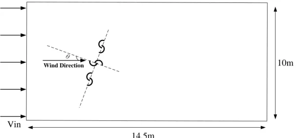
In this work, it is interesting to analyze the air flow field around one single rotating Savonius wind rotor firstly in conditions of different wind speeds and tip speed ratios by employing a CFD software, Fluent. Later, the studies of the parallel matrix system with three Savonius wind rotors in conditions of different wind speeds, tip speed ratios and phase angle differences are carried out. The influence of wind direction change on the parallel system is also studied.

The reference case in this work simulates the experimental one by Blackwell et al. [4]. The geometry of a two-bladed Savonius wind rotor is given in Fig. 1.4 and the corresponding information is summarized in Table 3.1.

Table 3.1 Geometry Information

Number of Blades 2

Height (m) 1

Diameter (m) 0.9 Overlap Ratio of Blades 0.15

In order to simulate the situations of the reference case and the two topics mentioned above, three types of rectangular domains are set as shown in Figs.

3.1, 3.2 and 3.3, respectively. The first type including one single Savonius wind

rotor inside the wind tunnel corresponds with the reference case; the second one is for the case of one single Savonius wind rotor in atmosphere; and the last is

(37)

22

for the case of three Savonius wind rotors rotating with the same angular speed and connected in parallel in atmosphere with fixed distance. The distance between the centers of two wind rotors is 1.2m. All the conditions consider both 2-D and 3-D simulations. The dimensions of these domains are listed in Table

3.2.

Table 3.2 Dimensions of Domains

Length Width Height (3-D) A Single Rotor Inside (Reference) 11.9m 4.6m 2m A Single Rotor in Atmosphere 14.5m 8m 2m Three-rotor in Atmosphere 14.5m 10m 2m

Furthermore, the domains including three Savonius wind rotors with different wind directions are set as shown in Fig. 3.4, and the angles of wind direction are 0°, ±15°, ±30° and ±45°. For simplification, it does not include the consideration of the shaft of wind rotors.

3.2 Governing Equations

In order to make the physical problem more tractable, some assumptions are made as follows:

1. The flow is incompressible.

(38)

23

3. Neglect the heat transfer and buoyancy effects.

Based on the assumptions mentioned above, the governing equations are given in the following.

3.2.1 The Continuity and Momentum Equation

Turbulent flows are characterized by fluctuating velocity field. In Reynolds averaging, the solution variables in the instantaneous (exact) Navier-Stokes equations are decomposed into the mean (ensemble-averaged or time-averaged) and fluctuating components. For the velocity components:

u_i = u_i + u_i′

(3-1) where u_i and u_i′ are the mean and fluctuating velocity components ( i = 1, 2, 3).

Likewise, for pressure and other scalar quantities:

ϕ = ϕ + ϕ′ (3-2) where ϕ denotes a scalar such as pressure, energy, or species concentration. Substituting expressions of this form for the flow variables into the instantaneous continuity and momentum equations and taking a time (or ensemble) average (and dropping the overbar on the mean velocity, u ) yields the ensemble-averaged momentum equations. They can be written in Cartesian tensor form as:

∂ρ ∂t + ∂ ∂xj ρui = 0 (3-3) ∂ ∂t ρui + ∂ ∂xj ρuiuj = − ∂P ∂xi + ∂ ∂xj μ ∂u_i ∂xj + ∂uj ∂xi − 2 3δij ∂u_l ∂xl + ∂ ∂xj(−ρui ′_u j′) (3-4)

Eq. (3-3) and (3-4) are called Reynolds-averaged Navier-Stokes (RANS) equations. They have the same general form as the instantaneous Navier-Stokes

(39)

24

equations, with the velocities and other solution variables now representing ensemble-averaged (or time-averaged) values. Additional terms now appear that represent the effects of turbulence. These Reynolds stresses, −ρu_i′u_j′, must be modeled in order to close Eq. (3-4).

3.2.2 RNG k-ε Model

The RNG-based k-ε turbulence model is derived from the instantaneous Navier-Stokes equations, using a mathematical technique called “renormalization group" (RNG) methods. The analytical derivation results in a model with constants different from those in the standard k-ε model. The additional terms and functions in the transport equations for k and ε are also different.

Transport Equations for the RNG k-ε Model

The turbulence kinetic energy, k, and its rate of dissipation, ε, are obtained from the following transport equations:

∂ ∂t ρk + ∂ ∂xi ρkui = ∂ ∂xj αkμeff ∂k ∂xj + Gk − ρε + Sk (3-5) and ∂ ∂t ρε + ∂ ∂xi ρεui = ∂ ∂x_j αεμeff ∂ε ∂x_j + C1ε ε k Gk − C2ερ ε2 k − Rε + Sε (3-6)

The term of Gk represents the production of turbulence kinetic energy.

From the exact equation for the transport of k, this term may be defined as G_k = −ρu_i′_u

j′ ∂u_∂xj

i. The quantities αk and αε are the inverse effective Prandtl numbers for k and ε, respectively. Sk and Sε are user-defined source terms.

(40)

25

Modeling the Turbulent Viscosity

The scale elimination procedure in RNG theory results in a differential equation for turbulent viscosity:

d ρ 2_k εμ = 1.72 ν ν 3−1+Cν dν (3-7) where ν = μ_eff/μ C_ν ≈ 100

Eq. (3-7) is integrated to obtain an accurate description of how the effective turbulent transport varies with the effective Reynolds number (or eddy scale), allowing the model to be better handled in the low-Reynolds-number and near-wall flows.

In the high-Reynolds-number limit, Eq. (3-7) gives μ_t = ρC_μk

2

ε (3-8)

with Cμ = 0.0845, derived using RNG theory.

RNG Swirl Modification

Turbulence, in general, is affected by rotation or swirl in the mean flow. The RNG model in FLUENT provides an option to account for the effects of swirl or rotation by modifying the turbulent viscosity appropriately. The modification takes the following functional form:

μ_t = μ_t0 f(α_s, Ω,k

ε) (3-9)

(41)

26

modification using either Eq. (3-7) or Eq. (3-8). Ω is a characteristic swirl number evaluated within FLUENT, and αs is a swirl constant that assumes

different values depending on whether the flow is swirl-dominated or only mildly swirling. This swirl modification always takes effect for axisymmetric, swirling flows and three-dimensional flows when the RNG model is selected. For mildly swirling flows (the default in FLUENT), αs is set to 0.07. For strong

swirling flows, however, a higher value of αs can be used.

Calculating the Inverse Effective Prandtl Numbers

The inverse effective Prandtl numbers, k and ε, are computed using the following formula derived analytically by the RNG theory:

α−1.3929 α0−1.3929 0.6321 _α+2.3929 α0+2.3929 0.3769 = μmol μ_eff (3-10)

where α0= 1.0. In the high-Reynolds-number limit μ_mol/μ_eff ≪ 1 , αk =

α_ε ≈ 1.393.

The Rε Term in the ε Equation

The main difference between the RNG and standard k-ε models lies in the additional term in the ε equation given by

R_ε=Cμρη 3_(1−η/η 0) 1+βη3 ε2 k (3-11) where η≡Sk/ε, η0=4.38, β=0.012.

The effects of this term in the RNG ε equation can be seen more clearly by rearranging Eq. (3-6). Using Eq. (3-11), the third and fourth terms on the right-hand side of Eq. (3-6) can be merged, and the resultant ε equation can be rewritten as

(42)

27 ∂ ∂t ρε + ∂ ∂xi ρεui = ∂ ∂xj αεμeff ∂ε ∂xj + C1ε ε k Gk + C3εGb − C2ε ∗ _ρε2 k (3-12) where C_2ε∗ is given by C_2ε∗ ≡ C_2ε+Cμη 3_{(1−η η} 0 ) 1+βη3 (3-13) In regions where η < η0, the R term makes a positive contribution, and C2ε∗

becomes larger than C2ε. In the logarithmic layer, for instance, it can be shown

that η ≈ 3.0 gives C_2ε∗ ≈ 2.0, which is close in magnitude to the value of C_2ε∗ in the standard k-ε model (1.92). As a result, for weakly to moderately strained flows, the RNG model tends to give results largely comparable to the standard k-ε model.

In regions of large strain rate (η > η0), however, the R term makes a

negative contribution, making the value of C_2ε∗ less than C2ε. In comparison

with the standard k-ε model, the smaller destruction of ε augments ε, reducing k and, eventually, the effective viscosity. As a result, in rapidly strained flows, the RNG model yields a lower turbulent viscosity than the standard k-ε model.

Thus, the RNG model is more responsive to the effects of rapid strain and streamlining curvature than the standard k-ε model, which explains the superior performance of the RNG model for certain classes of flows.

Model Constant

The model constants C1ε and C2ε in Eq. (3-6) have values derived analytically by the RNG theory. These values, used by default in FLUENT, are

C_1ε = 1.42, C_2ε = 1.68

3.2.3 Standard Wall Functions

(43)

28

Launder and Spalding (1974), and have been most widely used for industrial flows.

Momentum

The law-of-the-wall for mean velocity yields U∗ = 1 kln(Ey ∗_{) (3-14)} where U∗ ≡ UPCμ 1₄ kP12 τ_w ρ (3-15) y∗ ≡ρCμ 1 4_k_P12_y_P μ (3-16) In which

k = von Karman constant (=0.487) E = empirical constant (=9.793)

UP = mean velocity of the fluid at point P

KP = turbulent kinetic energy at point P

yP = distance from point P to the wall

μ = dynamic viscosity of the fluid

3.3 Boundary Conditions

In the model domain, there exist boundary conditions for the followings: rotation of the wind rotor, inlet surfaces, outlet surfaces, physical symmetric surfaces, and wall boundary conditions.

1. Rotation boundary condition

According to Eq. (2-3), the angular speed ω (rad/s) of the wind rotor is expressed as

(44)

29

ω = 2v1λ

D (3-23)

where D is the outer wind rotor diameter, ω the angular wind rotor speed, v1 the

wind velocity and λ the tip speed ratio.

2. The inlet boundary condition

The inlet boundary conditions are: u = u_in

v = 0 w = 0

where u, v and w represent the velocity components in X, Y and Z directions, respectively.

3. The outflow boundary condition

Out flow boundary conditions are used to model flow exits where the details of the low velocity and pressure are not known.

4. The symmetrical boundary conditions

They can be used to model zero-shear slip walls in viscous flows. These surfaces are not affected by frictions. (∂u

∂y = 0 )

5. Wall boundary conditions

The wall boundary conditions satisfy the no-slip condition (u, v, w =0) for velocity.

(45)

30

3.4 Introduction to FLUENT Software

FLUENT is a state-of-the-art computer program for modeling fluid flow and heat transfer in complex geometries. It provides complete mesh flexibility, including the ability to solve the flow problems using unstructured meshes that can be generated about complex geometries with relative ease. Supported mesh types include 2D triangular/quadrilateral, 3D tetrahedral/hexahedral/pyramid, and mixed (hybrid) meshes. FLUENT also allows refining or coarsening grid based on the flow solution.

FLUENT is written in the C computer language and makes full use of the flexibility and power offered by the language. Consequently, true dynamic memory allocation, efficient data structures, and flexible solver control are all possible. In addition, FLUENT uses a client/server architecture, which allows it to run as separate simultaneous processes on client desktop workstations and powerful compute servers. This architecture allows for efficient execution, interactive control, and complete flexibility between different types of machines or operating systems.

All functions required to compute a solution and display the results are accessible in FLUENT through an interactive, menu-driven interface.

3.5 Numerical Method

This study employs the computational fluid dynamics software Fluent to analyze the flow fields around rotating Savonius wind rotors. The finite volume iteration and SIMPLE algorithm are put in use to solve the governing equations of a transient flow field. And the corresponding grid movement is also solved by using sliding mesh method.

(46)

31

FLUENT uses Segregated Solver method to solve the governing integral equations for the conservation of mass and momentum, and (when appropriate) for energy and other scalars such as turbulence and chemical species. In case a control-volume-based technique is used that consists of:

 Division of the domain into discrete control volumes using a computational grid.

 Integration of the governing equations on the individual control volumes to construct algebraic equations for the discrete dependent variables such as velocities, pressure, temperature, and conserved scalars.

 Linearization of the discretized equations and solution of the resultant linear equation system to yield updated values of the dependent variables.

3.5.1 Segregated Solution Method

Using this approach, the governing equations are solved sequentially (i.e., segregated from one another). Because the governing equations are non-linear (and coupled), several iterations of the solution loop must be performed before a converged solution is obtained. Each iteration consists of the steps illustrated in

Fig. 3.5 and outlined below:

1. Fluid properties are updated, based on the current solution. (If the calculation has just begun, the fluid properties will be updated based on the initialized solution.)

2. The u, v, and w momentum equations are each solved in turn using current values for pressure and face mass fluxes, in order to update the velocity field. 3. Since the velocities obtained in Step 2 may not satisfy the continuity equation locally, a Poisson-type equation for the pressure correction is derived from the continuity equation and the linearized momentum equations. This

(47)

32

pressure correction equation is then solved to obtain the necessary corrections to the pressure and velocity fields and the face mass fluxes such that continuity is satisfied.

4. Where appropriate equations for scalars such as turbulence, energy, species, and radiation are solved using the previously updated values of the other variables.

5. When interphase coupling is to be included, the source terms in the appropriate continuous phase equations may be updated with a discrete phase trajectory calculation.

6. A check for convergence of the equation set is made.

These steps are continued until the convergence criteria are met.

3.5.2 Linearization: Implicit

In the segregated solution method the discrete, non-linear governing equations are linearized to produce a system of equations for the dependent variables in every computational cell. The resultant linear system is then solved to yield an updated flow-field solution.

The manner in which the governing equations are linearized may take an implicit form with respect to the dependent variable (or set of variables) of interest.

The implicit form is described in the following:

 Implicit: For a given variable, the unknown value in each cell is computed using a relation that includes both existing and unknown values from neighboring cells. Therefore each unknown will appear in more than one equation in the system, and these equations must be solved simultaneously to give the unknown quantities.

(48)

33

In the segregated solution method each discrete governing equation is linearized implicitly with respect to that equation's dependent variable. This will result in a system of linear equations with one equation for each cell in the domain. Because there is only one equation per cell, this is sometimes called a scalar system of equations. A point implicit (Gauss-Seidel) linear equation solver is used in conjunction with an algebraic multigrid (AMG) method to solve the resultant scalar system of equations for the dependent variable in each cell. For example, the x-momentum equation is linearized to produce a system of equations in which u velocity is the unknown. Simultaneous solution of this equation system (using the scalar AMG solver) yields an updated u-velocity field.

In summary, the segregated approach solves for a single variable field (e.g., p) by considering all cells at the same time. It then solves for the next variable field by again considering all cells at the same time, and so on. There is no explicit option for the segregated solver.

3.5.3 Discretization

FLUENT uses a control-volume-based technique to convert the governing equations to algebraic equations that can be solved numerically. This control volume technique consists of integrating the governing equations about each control volume, yielding discrete equations that conserve each quantity on a control-volume basis.

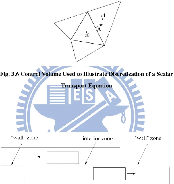
Discretization of the governing equations can be illustrated most easily by considering the steady-state conservation equation for transport of a scalar quantity ϕ. This is demonstrated by the following equation written in integral form for an arbitrary control volume V as follows:

(49)

34 ρϕv ∙ dA = Γ_ϕ∇ϕ ∙ dA + S_V _ϕdV (3-24) where ρ = density v = velocity vector A

= surface area vector

Γ_ϕ = diffusion coefficient for ϕ ∇ϕ = gradient of ϕ

S_ϕ= source of ϕ per unit volume

Eq. (3-24) is applied to each control volume, or cell, in the computational domain. The two-dimension, triangular cell shown in Fig. 3.6 is an example of such a control volume. Discretization of Eq. (3-24) on a given cell yields

N_f faces ρ_fv ϕ_f _f ∙ A =_f _fNfaces Γ_ϕ(∇ϕ)_n ∙ A + S_f _ϕV (3-25) where

Nfaces = number of faces enclosing cell

ϕ_f = value of ϕ convected through face f

ρ_fv _f∙ A = mass flux through the face _f

A = area of face f f

(∇ϕ)_n = magnitude of ∇ϕ normal to face f V = cell volume

The equations solved by FLUENT take the same general form as the one given above and apply readily to multi-dimension, unstructured meshes composed of arbitrary polyhedral.

By default, FLUENT stores discrete values of the scalar ϕ at the cell center (c0 and c1 in Fig. 3.6). However, face values ϕ_f are required for the

(50)

35

convection terms in Eq. (3-25) and must be interpolated from the cell center values. This is accomplished using an upwind scheme.

First-Order Upwind Scheme

When first-order accuracy is desired, quantities at cell faces are determined by assuming that the cell-center values of any field variable represent a cell-average value and hold throughout the entire cell; the face quantities are identical to the cell quantities. Thus when first-order upwind is selected, the face value ϕ_f is set equal to the cell-center value of ϕ in the upstream cell.

3.5.4 SIMPLE Algorithm

The SIMPLE algorithm uses a relationship between velocity and pressure corrections to enforce mass conservation and to obtain the pressure field.

If the momentum equation is solved with a guessed pressure field p*, the resulting face flux J_f∗, computed from J_f = J _f + d_f(p_c0 − p_c1) (where pc0 and pc1

are the pressures within the two cells on either side of the face, and J _f contains the influence of velocities in these cell. The term df is a function of ap, the

average of the momentum equation a_p coefficients for the cells on either side of face f.)

J_f∗ = J ∗

f + df(pc0∗ − pc1∗ ) (3-26)

does not satisfy the continuity equation. Consequently, a correction J_f′ is added to the face flux J_f∗ so that the corrected face flux, J_f

J_f = J_f∗ + J_f′ (3-27) satisfies the continuity equation. The SIMPLE algorithm postulates that J_f′

(51)

36

be written as

J_f′ = d_f(p_c0′ + p_c1′ ) (3-28) where p′ is the cell pressure correction.

The SIMPLE algorithm substitutes the flux correction equations, Eq. (3-27) and (3-28), into the discrete continuity equation ( N_f faces J_fA_f = 0) to obtain a discrete equation for the pressure correction p′ in the cell:

a_pp′ = a_nb _nbp_nb′ + b (3-29) where the source term b is the net flow rate into the cell:

b = N_f faces J_f∗A_f (3-30) The pressure-correction equation, Eq. (3-29), may be solved using the algebraic multigrid (AMG) method. Once a solution is obtained, the cell pressure and the face flux are used correctly.

p = p∗ + α_pp′ (3-31) J_f = J_f∗+ d_f(p_c0′ − p_c1′ ) (3-32) Here α_p is the under-relaxation factor for pressure. The corrected face flux J_f satisfies the discrete continuity equation identically during each iteration.

3.5.5 Sliding Mesh

The sliding mesh model allows adjacent grids to slide relative to one another. In doing so, the grid faces do not need to be aligned on the grid interface. This situation requires a means of computing the flux across the two non-conformal interface zones of each grid interface.

To compute the interface flux, the intersection between the interface zones is determined at each new time step. The resulting intersection produces one

(52)

37

interior zone (a zone with fluid cells on both sides) and one or more periodic zones. If the problem is not periodic, the intersection produces one interior zone and a pair of wall zones (which will be empty if the two interface zones intersect entirely), as shown in Fig. 3.7. The resultant interior zone corresponds to where the two interface zones overlap; the resultant periodic zone corresponds to where they do not. The number of faces in these intersection zones will vary as the interface zones move relative to one another. Principally, fluxes across the grid interface are computed using the faces resulting from the intersection of the two interface zones, rather than from the interface zone faces themselves.

In the example shown in Fig. 3.8, the interface zones are composed of faces A-B and B-C, and faces D-E and E-F. The intersection of these zones produces the faces a-d, d-b, b-e, etc. Faces produced in the region where the two cell zones overlap (d-b, b-e, and e-c) are grouped to form an interior zone, while the remaining faces (a-d and c-f) are paired up to form a periodic zone. To compute the flux across the interface into cell IV, for example, face D-E is ignored and faces d-b and b-e are used instead, bringing information into cell IV from cells I and III, respectively.

3.6 Computational Procedure of Simulation

The complete operating procedure for using FLUENT package software is carried out through the following processes sequentially.

3.6.1 Model Geometry

For FLUENT calculations, it is necessary to build a model firstly. This study used the pre-processor software Gambit to build the case study model. It

(53)

38

has to divide the case study into finite volumes in this step in order to generate grids conveniently. The details of geometry information can be referred in Section 3.1.

3.6.2 Grid Generation

After building the case study model, it has to use the pre-processor Gambit to generate grids as shown in Fig. 3.9. It defines the different grid sizes in different volumes in this step. Defining the smaller grid size for the smaller volume will increase the accuracy of the simulation, but it must consider the applicability of the grid size. If it adopts too small grid size in this step, the simulation time will be influenced. Besides, if the largest grid size is different from the smallest one too much, it will influence the FLUENT calculation.

3.6.3 FLUENT Calculation

Once determine the important features of the problem that one wants to solve, it will follow the basic procedural steps shown below.

1. Create the model geometry and grid.

2. Start the appropriate solver for 2D or 3D modeling. 3. Import the grid.

4. Check the grid.

5. Select the solver formulation.

6. Choose the basic equations to be solved: laminar or turbulent (or inviscid), chemical species or reaction, heat transfer models, etc. Identify additional models needed: fans, heat exchangers, porous media, etc.

7. Specify material properties. 8. Specify the boundary conditions.