Tobin's Q與住宅投資:台灣的實證分析

行政院國家科學委員會專題研究計畫 成果報告

Tobin，s Q 與住宅投資:台灣的實證分析

中 華 民 國 95 年 6 月 19 日

TOBIN’S Q AND HOUSING INVESTMENT: THE CASE OF TAIWAN*

Chu-Chia Lin** November 2005

Abstract

The purpose of this paper is to test the famous Tobin (1969) Q theory in explaining housing investment behavior of Taiwan. Defining Tobin’s Q as the ratio of pre-sale housing price to rental housing price, we check the cointegration relation between Tobin’s Q and housing investment (both for construction permits and for building permits) first. In order to estimate the effect of Tobin’s Q on housing investment, we also put on two major housing production costs as explanatory variables, namely interest rate and wage rate of construction workers. Applying a quarterly housing data set of Taiwan from 1982 to 2003, we find that Tobin’s Q does have a significant effect on number of construction permits. However, the coefficient of Tobin’s Q on number of building permits is insignificant. Moreover, prime rate and wage rate also have significant effect on housing investment.

Key Words: Tobin’s Q, housing investment, Taiwan

* _{The author thanks comments from the participants of the 2005 Annual Conference on the Chinese} Society of Housing Studies, Dec.4, 2004, Taipei. The author also thanks financial support from National Science Fundation (NSC93-2415-H004-016).

** _{Professor, Department of Economics, National Chengchi University, Taipei, Taiwan, 116. E-mail:}

1. Introduction

Tobin (1969) argues that the size of investment for a certain firm depends on the ratio of the value of its current asset with its replacement cost. Following Tobin’s seminal paper, there are lots of literature discussing Tobin’s Q theory, both in theory and in empirical study, such as Hayashi (1982), Wildasin (1984), and Caballero and Leahy (1996).

Housing investment is an important investment behavior, both for households and for housing constructors. Now, the question is whether Tobin’s Q applies on housing investment behavior. The answer for this question is important not only on academic purpose, but it has an important policy implication. If Tobin’s Q is good in explaining housing investment behavior, then we could use this theory to explain the accumulation of housing stock for a society.

For an ordinary machine, since the replaced machine could be exactly the same as the old one, it will be easy to identify the value of the used machine. If the new machine has a better function with higher efficiency, then we could estimate cash flow and net present value of the new machine, so the actual Tabin’s Q could be correctly estimated. However, the situation for housing investment is quite different. Since there are so many attributes for each dwelling unit, including floor space, location, construction material, and so on, the housing unit should be standardized before we calculate its investment value and its replacement cost.

Owing to lack of data, there is little literature discussing the importance of Tobin’s Q on housing investment. Until recent years, there are some literatures studying the Tobin’s Q on housing investment. Takala and Tuomala (1990) study the relation of Tobin’s Q on housing investment applying a data set from Dutch housing market, and they find that Tobin’s Q does have a significant effect on housing investment. Jud and Winkler (2003) is the first paper applying time series analysis on the relation of Tobin’s Q and housing investment. Applying a data set from the housing market of the US, they get same results as Takala and Tuomala (1990).

There is little study on Tobin’s Q theory in Taiwan. Hsu (1985) may be the first paper studying this topic. Moreover, there is little empirical study since the data set on real return of machines and equipments are difficult to get. However, there are some articles in financial literature mainly because that the financial data are easier to get, including Yu and Chen (1999), Lin and Hsu (1999), Lin and Peng (1998), Hsieh and Chang (1995), Yu and Chou (1994), and Hsieh (1994, 1995). Wang (2000) may

be the first paper applying Tobin’s Q on the manufacturing firms of Taiwan. Wang (2000) uses different methods to measure the size of Tobin’s Q for manufacturing firms in Taiwan, and then he estimates the effect of Tobin’s Q on investment.

Since housing investment is a very important investment behavior both for households and realtors in Taiwan, it is crucial to know whether Tabin’s Q works in Taiwan’s housing market. Therefore, the purpose of this paper is to test whether Tobin’s Q is good to explain housing investment behavior in Taiwan. Following Jud and Winkler (2003), we employ time series method to analyze the relation of Tobin’s Q and housing investment. Moreover, in order to correctly estimating the coefficient of Tobin’s Q on housing investment, we also put two key variables on housing construction cost, namely interest rate and wage rate of construction workers. Since this is the first paper in Taiwan studying the effect of Tobin’s Q on housing investment behavior, the findings of this study could provide us better prediction on housing investment, and the findings could also provide us a better understanding on the relation of housing quantity and housing prices.1

The structure of this paper is as follow: Section 2 states the theoretical relation of Tobin’s Q and housing investment. The data set and definitions of variables are explained in Section 3. In Section 4, we will apply the time series analysis method to estimate the coefficients of Tobin’s Q, interest rate, and wage rate on housing investment. This study is concluded in Section 5.

2. Tobin’s Q and Housing Investment

By Tobin (1969)’s definition, Qt represents a ratio of the market value (MVt) at time t for a certain machine (or a certain capital), or its marginal productivity, to its replacement cost (RCt). When the market value (or marginal productivity) exceeds its replacement cost, then it is profitable to invest and so the firms should increase its investment. On the other hand, if a machine’s market value is less than its replacement cost, then it is not profitable to invest and so the firm should cut its investment. So, t t t M V ( 1 ) Q = R C

1 _{These is a typical saying in the housing market of Taiwan that the changes of quantity index of} housing transaction is always ahead of the changes of housing price, for instance, Hwa and Chang (1999). This study provides us a chance to test this statement.

The market value (MVt) of the machine (or capital) could be calculated by discounting with market interest rate (it) on its cash flow (rt) generated by this machine, i.e. net present value.2 In order words,

T j t j t j = t t r ( 2 ) M V = ( = N P V ) ( 1 + i )

∑

There are two ways to estimate the replacement cost: One is to apply the actual replacement cost for the machine in question, i.e. marginal cost (MCt). Moreover, if the production function is constant return to scale, then we could use average cost (ACt) to represent MCt since MCt=ACt when the production is constant return to scale. Another way is to use the user cost, or rental cost (Rt), to represent replacement cost, i.e. t t ( 3 ) R C = M C Or t t ( 4 ) R C = R

In the housing market, whether the realtors like to invest or not depends upon the difference of housing price (price expectation) between new dwelling units (or pre-sale houses) and existing houses. For instance, if a housing constructior expects that the price of pre-sale houses is relatively high, or the price of existing houses is lower, then this constructor will start to invest in pre-sale houses. Therefore, the housing investment will increase. On the contrary, if the constructor expects that the price of pre-sale houses is relatively low, then he will choose not to build pre-sale houses. Thus, the housing investment will decrease. However, the investment behavior for households is different. When a household expects that the average price of pre-sale houses is relatively higher, or the average price of existing houses is lower, then he will prefer to buy the existing houses, but not to buy the pre-sale houses. Therefore, the household’s investment in new housing stock will be smaller.3

Moreover, if the housing market is efficient, then the price of pre-sale houses

2 _{Here we assume that there is no capital gain.}

3 _{In Taiwan, since investment in pre-sale housing stocks and the pre-sale housing price are mainly} determined by the constructors, we expect that construction permits will be more sensitive to Tobin’s Q. On the other hand, building permits are owned by the households and so are less responsive to Tobin’s Q.

(PHt) could represent the net present value (NPVt) for new housing investment;4 while the price for the existing houses represents returns of replacement cost.5

Moreover, if we use user cost to represent marginal cost of the existing houses and if the housing market is efficient, the housing rent could represent housing price for the existing houses.6 Therefore, we could use rental cost (Rt) for the price existing houses. Finally, we define Tobin’s Q as follow:

(5) t t t R PH Q =

To estimate the impact of Q ratio on housing investment in Taiwan, we follow Jud and Winkler (2003)’s paper in that the amount of housing investment (It) is determined by the Q ratio for the past years, i.e.

(6) I_t =f(Q_t,Q_t−1,")

By Jud and Winkler (2003), Tobin’s Q should have a positive effect on housing investment (It). Moreover, the effect would have time lag since it takes time to build a dwelling unit.7 This positive effect implies that the relative housing price will affect housing investment because the movement of the relative housing price is faster than the construction speed for housing units.

To correctly estimate the effect of Q ratio on housing investment, we put two more explanatory variables in Equation (6), namely, prime rate and wage rate of construction workers. These two variables are crucial for construction cost and thus should have significant effect on housing investment, especially for housing constructors. Without considering these important variables, the estimated coefficient of Q ratio on housing investment could be seriously biased.8 Therefore, we could

4 _{In Taiwan, the pre-sale housing price is mainly determined by the housing constructors, which} represent the constructors’ returns of investment, or market value.

5 _{See Meese and Wallace (1995) and Rosenthal (1999).}

6 _{We could also apply the traditional way to calculate user cost for the existing houses, including rent,} depreciation cost, tax rate, maintenance cost, and so on. For example, Poterba (1991), Haurin, et al (1994), and Chen and Lin (2002).

7 _{In general, it takes 18 months to build a five-floor apartment and it takes 30 months to build a} twelve-floor building in Taiwan.

8 _{According to traditional econometric theory, missing some important explanatory variables could} generate seriously bias for the existing explanatory variables. However, whether the bias is up-ward

rewrite Equation (6) as follow:

(7) I_t =f(Q_t,PR_t,WAGE_t,Q_t−1,PR_t−1,WAGE_t−1,")

3. Data Description

The quarterly data set applied in this study is from the first quarter of 1982 to the last quarter 2003, so there are 88 observations for each variable. All variables come from Real Estate Cycle Indicators of Taiwan, published by Institute of Construction, Department of Interior Affairs, ROC, and Taiwan Real Estate Study Center, National Chengchi University.9

Definitions of Variables:

BP: total floor space of building permits, unit: ten thousand square meters. CP: total floor space of construction permits, unit: ten thousand square meters. PH: index for the average price of pre-sale and new housing units per pin with the

base year of 2000.10

PR: prime rate of Bank of Taiwan, unit: %. Q Ratio: the ratio of PH to RT.

RT: index for rental price with the base year of 2000.

WAGE: the average monthly wage of construction industry, unit: NT$.

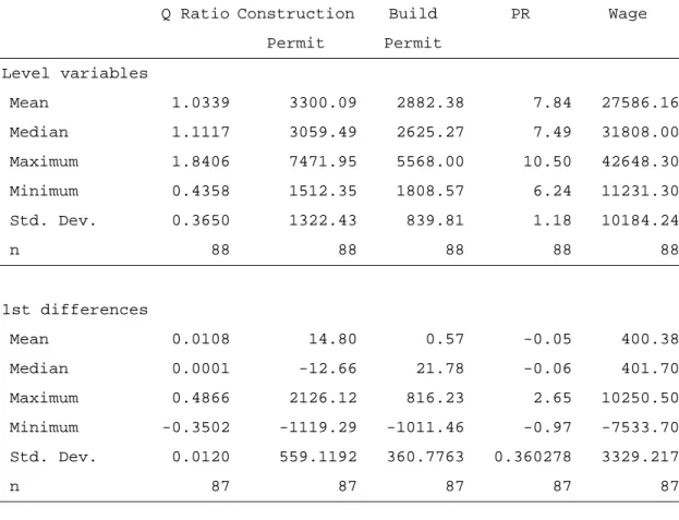
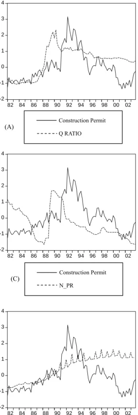
Table 1 shows that the average ratio of Q is 1.0339 with a small deviation (0.365). It looks like Taiwan has a stable Q ratio in the past twenty years, but the fact is that there was a sharp change in Q ratio. As shown in Figure 1(A), Q ratio was stable around 0.50 before 1986 and then it quickly jumped up to 1.80 in 1989 and reached its peak on Q2, 1990. And then it gradually drops. Construction permits and building permits have shown similar patterns. Total number of floor space of construction permits was increased at a slow speed before and then suddenly jumped up in Q2, 1991,11 which was exactly one year after the Q ratio reached it peak. The amount of construction permits reached its peak on Q2, 1992. At the same time, the total floor space of build permits shows a similar pattern but with time lag. Figure 1(C) shows that total number of building permits started sharply increasing on Q2, 1992, one year after construction permits starting to increase. Moreover, the

or down-ward depends upon the correlation of the missing variables and the existing variables and the coefficient of the existing variables on the explained variable. See Maddala (2001), p.159-161. 9 _{The author appreciates Professor C.O. Chang kindly providing the original data set for this study.} About the details of data set, please see the Appendix.

10 _{One pin equals 36 square foot.}

building permits reached its peak on Q3, 1994, which was two years after the construction permits reaching its peak.

[Put Table 1 here.] [Put Figure 1 here.]

The trend of prime rate (PR) of bank loan has a different pattern, but tells a same story in Taiwan. Figure 1(D) shows that the prime rate was continuously decreasing from (9.80%) in Q1, 1982 to its bottom (6.24%) in Q2, 1988. Thereafter, the prime rate suddenly jumped to 9.40% in Q2, 1989, and reached its peak in the next quarter. And then it started to drop two years later and till now. The ups and downs of prime rate of Taiwan shows the story of downs and ups of housing market in Taiwan. When the prime rate kept dropping before 1988, it provided people in Taiwan a good incentive to invest in housing market. But when the housing price had started to sharply increase since Q3, 1988, Taiwan government tried to use monetary policy to cool down the housing market and so the prime rate started to grow. As the housing price was stable in Taiwan after Q3, 1990, Taiwan government started to let the prime rate go down gradually.

The monthly wage rate of Taiwan has been increasing slowly since Q1, 1982, with a stable rate. When the housing market was hot around 1990, the wage rate of construction industry was still stable. On the other hand, when the housing market was in a recession after 1990, the wage rate was still increasing at a stable rate till now. In Figure 1(E), the reason why there is a spike in every year is because that the yearly bonus is distributed in the first quarter in each year.12

Figure 2 shows the co-movements of key variables. In Figure 2(A) and 2(B), we could see that the movement of Q ratio is leading the movements of construction permits and building permits. On the other hand, we also see the movement of prime rate has a reverse movement with both construction permits and building movements in Figure 2(C) and 2(D). However, the pattern of co-movement of wage and construction is not that clear, neither the co-movement between wage and building permits. Figure 1 and 2 provide us some preliminary results about the correlation among key variables. Now, we want to employ a time-series analysis method to find out the exact relation between Q ratio and housing investment. [Put Figure 2 here.]

12 _{In order to deal with the serious seasonal deviation problem, we apply a seasonal adjustment method} to smooth the seasonal data and we also use the adjusted quarterly data to re-run our regression.

4. Empirical Results

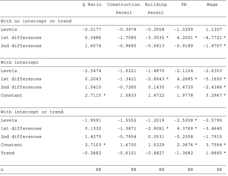
In order to check if there exists a unit root for each time-series variable, the Augmented Dickey-Fuller tests were conducted first in Table 2. Following Jud and Winkler (2003), the tests were conducted with two lagged first differences and employed three specifications of the test equation: (1) no intercept or trend, (2) intercept, and (3) intercept and trend. Table 2 shows that all of the variables have unit roots in levels, but not in 1st or 2nd differences.13 The result shows that traditional OLS is inappropriate for this non-stationary series because the regression residual will also be non-stationary.

[Put Table 2 here.]

Following Johansen (1995) and Jud and Winkler (2003), we then conducted a series of cointegration tests using Q ratio, PR, and WAGE as explanatory variables. Here, we use two types of housing investment measurements: One is total floor space of construction permits (CPt), the other one is total floor space of building permits (BPt). The Johansen procedure considers five alternative assumptions regarding the presence of intercept and trend in the tests, and the test vector autoregression (VAR) equation is estimated with two time lags. The results of the cointegration test are shown in Table 3. Table 3 shows that the null hypothesis of no integration is not rejected at 1% significance level in any of the tests.

[Put Table 3 here.]

Since the variables are not cointegrated but do have unit roots in level, we conclude that the basic model in Equation (7) could be estimated in the first-difference form as follow:

(8) ΔI_t = Δf( Q ,ΔPR ,ΔWAGE ,ΔQ ,ΔPR ,ΔWAGE , )_{t t t t 1− t 1− t 1−} "

To estimate Equation (8), three periods of lags are employed in order to get the maximum adjusted R-squares of the estimated investment equation. Moreover, we use both construction permits (CPt) and building permits (BPt) as proxy variables for housing investment. Applying the ordinary least squares (OLS) method, the estimated results are reported in Table 4. In the construction permits in Table 4, one could see

13 _{In the Augmented the Dickey-Fuller unit root test, the null hypothesis is that the time series is not} stationary, i.e. there exists a unit root.

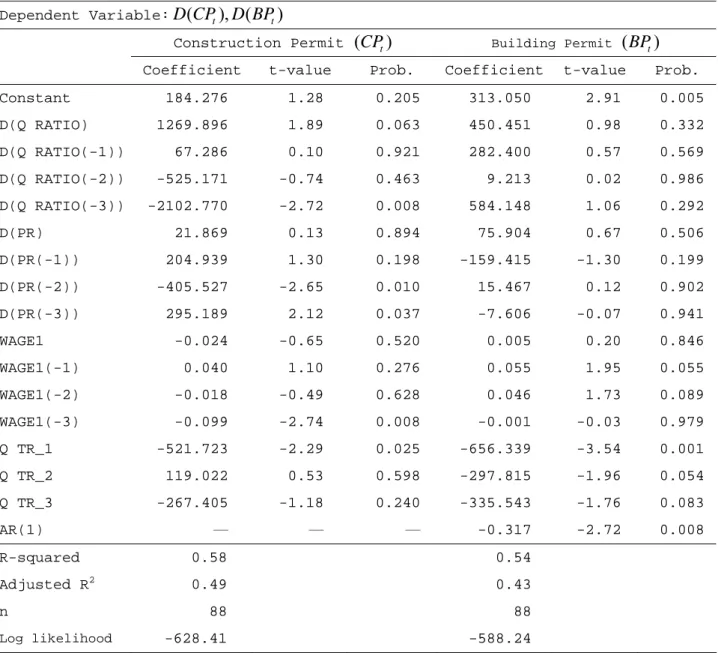
that the Q ratio does have a positively significant effect on CPt (1269.896) for the variable D(Q ratio). The result confirms our hypothesis that Q ratio has a positive effect on housing investment and the increment comes from the same period, which means that the housing constructors have a quick response to the housing market. However, D(Q ratio(-3)) has a negative coefficient (2102.770). Since the significant and negative effect on coefficient happens one year later, it could be caused by the lag response of rental price.

[Put Table 4 here.]

Meanwhile, D(PR(-2)) has a negatively significant sign (-405.527) which is consistent with our expectation since the prime rate of bank loan is an important cost for housing investment. Moreover, WAGE (-3) has a negatively significant coefficient (-0.099) which is again consistent with our expectation since labor cost is another important cost for housing construction.

The estimation results for building permits are quite different from construction permits. In Table 4, one could see that the coefficients of Q ratio and PR are not significant at all, which shows that Q ratio and prime rate have no effect on building permits at all. Moreover, there are two significant coefficients for WAGE(-1) and WAGE(-2) with wrong signs. There are two possible reasons to explain the different estimated results for construction permits and for building permits: One is that we may have to take more periods of lag variables since building permits have much longer time lag comparing to construction permits. The other reason is that, since building permits are more related with households’ investment behavior while construction permits are more related with constructors’ investment behavior, and the latter is less responsive to the housing market than construction permits.

One of important implications in our findings here is that, since Tobin’s Q does have a significant impact on number of construction permits, the pre-sale housing price has impact on housing stock (or at least on pre-sale housing stock). It means that housing price is moving ahead of housing quantity only for construction permits. But, since the pre-sale housing price has no effect on the building permits, it implies that housing price is not moving ahead of building housing permits.

Since the quarterly dummies have significant signs, it implies that there is a discrepancy among different seasons in Taiwan’s housing market. So we also apply

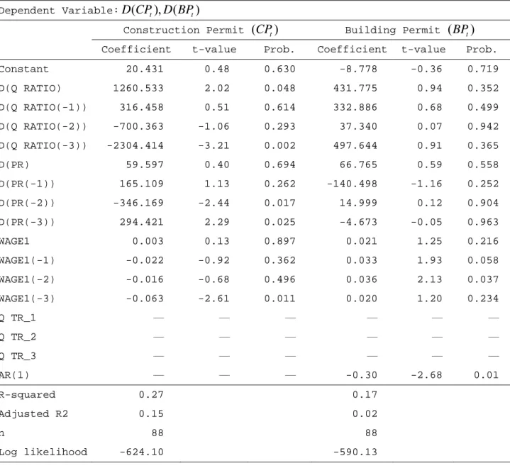
seasonal adjustment method to smooth the quarterly time series data.14 The estimation results with seasonal adjustment are reported in Table 5. The estimation results in Table 5 are quite similar to the results in Table 4. Almost all independent variables have same sings and significance both for construction permits equation and for building permits equation. The result shows that our regression result is robust.

[Put Table 5 here.]

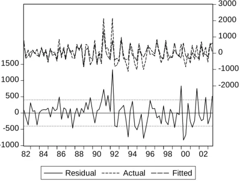
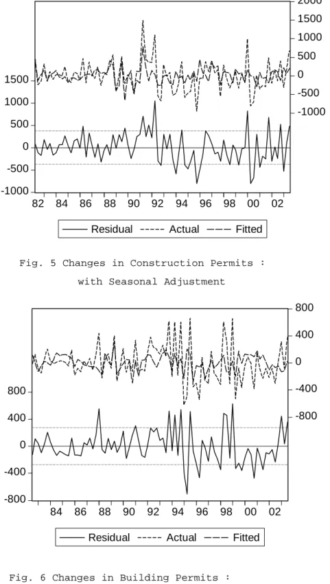
Finally, we plot the estimated residuals (together with actual and fitted residuals) for the estimated equations both for construction permits and for build permits in Table 4 and Table 5 as in Figure 3、4、5、and 6. Since there is no vivid pattern in those figures, it implies that our OLS regression setting is ok here.

[Put Figure 3、4、5、6 here.]

5. Conclusion

This study applies a time series data set from Taiwan’s housing market to test whether Tobin’s Q theory could explain housing investment behavior in Taiwan. Defining Q ratio as the ratio of the price of pre-sale house to the price of rental cost, we found that Q ratio is positively related with housing investment on the amount of floor space for construction permits. However, Q ratio has no effect on housing investment on building permits. In other words, while construction permits quickly responses to Q ratio, building permits is not responsive to Q ratio for its long construction lag. This result is different from Jud and Winkler (2003)’s findings in the US housing market.15 Moreover, prime rate and construction labor cost also have significant effects on housing investment on construction permits, but not on building permits.

Owing to lack of data, this study only provides one way to calculate Q ratio. Since Q ratio is crucial for estimating housing investment behavior, it is worthwhile to compute Q ratios by different definitions for future study.

14 _{The seasonal adjustment method applied here is the ratio to moving average-multiplicative method.} See Eview 4 User’s Guide, 2002, p.189-190.

15 _{One reason why that building permits (BPt) are responsive to Q ratio in Jud and Winkler (2003) but} not in our study is that we use the pre-sale price to define Q ratio and so BPtis less responsive to it in Taiwan.

References:

Caballero, R.J., and J.V. Leahy (1996), “Fixed Costs: The Demise of Marginal q,” Working Paper No. 5508, NBER.

Chen, C.L, and C.C. Lin (2002), “Choice of Mortgage Payment and of Tenure Choice,” Paper Presented at the AsRES/AREUEA International Conference, Seoul, Korea, July 2002.

Haurin, D.R., P.H. Hendershott, and S.M. Wachter (1995),”Wealth Accumulation and Housing Choices of Young Households: An Exploratory Investigation,” Working Paper No. 5057, NBER.

Hayashi, F. (1982), “Tobin’s q and Average q: A Neoclassical Interpretation,’ Econometrica, 50, 213-224.

Hsieh, C.P. (1994), “The Impact of the Announcement of Capital Expenditure on the Wealth of Stockholders: A Test on the Hypotheses of Jensen’s Excess Cash Flow and Tobin’s Q,” Journal of Financial Studies , 1(2), 37-52. (in Chinese)

Hsieh, C.P. (1995), “Applying Tobin’s Q to Estimate the Responsiveness of Stock Price on the Changes of Company’s Investment,” Management Review, 14(1), 33-45. (in Chinese)

Hsieh, C.P., and C.C. Chang (1996), “A Study on the Relation of Firm’s Decision of M&A and Tobin’s Q on Taiwan,” Quarterly Review of Bank of Taiwan, 47(3), 35-55. (in Chinese)

Hsu, C.M. (1985), “Tobin’s Q Theory and Optimal Allocation of Investment Goods in a Two-Sector Model,” Taiwan Economic Review, 13, 87-118.

Hwa, G.C., and C.O. Chang (1999), “The Relation of Price and Quantity for Pre-Sale Houses and Existing Houses for the Sub-Market: Reviewing the Effectiveness of the Policy on Reviving the Construction Industry,” The Proceedings of the 8th

Annual Conference of the Society of Housing Study of Taiwan, 27-42. (in Chinese) Johansen, S. (1995), Likelihood-based Inference in Cointergration Vector

Autoregressive Models, Oxford University Press, Oxford.

Jud, G. D., and D. T. Winkler (2003), “The Q Theory of Housing Investment,” Journal of Real Estate Finance and Economics, 27(3), 379-392.

Lin, I. M., and C.I. Peng (1999), “The Content of the Announcement of Stock Dividend ad Tobin’s Q Theory,” Journal of Management, 15(4), 587-621. (in Chinese)

Lin, S. H., and C.C. Hsu (1999), “An Empirical of the Relation of Complicate Tobin’s Q and Simple Tobin’s Q,” Managerial Accounting, 47, 66-76. (in Chinese)

Maddala, G.S. (2001), Introduction to Econometrics, 3rd ed, John Wiley and Sons, LTD, NY.

Meese, R., and N. Wallace (1994), “Testing the Present Value Relation of Housing Prices: Should I Leave My House in San Franscisco,” Journal of Urban Economics, 35, 245-266.

Poterba, J. (1991), “House Price Dynamics: The Role of Tax Policy and Demography,” Brookings Papers on Economic Activity, 2, 143-183.

Rosenthal, S.S. (1999), “Residential Buildings and the Cost of Construction: New Evidence on the Efficiency of the Housing Market,” The Review of Economics and Statistics, 81, 288-302.

Schaller, H.(1990), “Re-Examination of the Q Theory of Investment Using U.S. Farm Data,” Journal of Applied Econometrics, 5, 309-325.

Summerville, C.T.(1999), ”Residential Construction Costs and the Supply of New Housing: Endogeneity and Bias in Construction Cost Indexes,” Journal of Real Estate Finance and Economics, 18,43-62.

Summers, L.H. (1981), ”Taxation and Corporate Investment: A q-Theory Approach,” Brookings Papers and Economic Activity, 1, 67-127.

Takala, K., and M. Tuomala (1990), “Housing Investment in Finland,” Finish Economic Papers, 3, 41-53.

Tobin, J. (1969), “A General Equilibrium Approach to Monetary Theory,” Journal of Money, Credit, and Banking, 1, 15-29.

Wang, H.J.(2000), “Estimating the Tobin’s Q for Individual Firms in Taiwan,” Academia Economic Papers, 28(2), 149-176. (in Chinese)

Wildasin, D. (1984), “The q Theory of Investment with Many Capital Goods,” American Economic Review, 74, 203-210.

Yu, H.C., and H.C.Chen (1999), “A Study on the Relation of the Growth Rate, Leverage, and Tobin’s Q for the Stock Listing Companies of Taiwan,” Journal of Risk Management, 1(1), 81-101. (in Chinese)

Yu, H.C., and P.E. Chou (1994), “A Study on the Relation of Board Members’ Stock Holding Share and Company’s Tobin’s Q,” Management Review, 13(1), 79-98. (in Chinese)

Table 1 Descriptive Statistics

Q Ratio Construction Build PR Wage

Permit Permit Level variables Mean 1.0339 3300.09 2882.38 7.84 27586.16 Median 1.1117 3059.49 2625.27 7.49 31808.00 Maximum 1.8406 7471.95 5568.00 10.50 42648.30 Minimum 0.4358 1512.35 1808.57 6.24 11231.30 Std. Dev. 0.3650 1322.43 839.81 1.18 10184.24 n 88 88 88 88 88 1st differences Mean 0.0108 14.80 0.57 -0.05 400.38 Median 0.0001 -12.66 21.78 -0.06 401.70 Maximum 0.4866 2126.12 816.23 2.65 10250.50 Minimum -0.3502 -1119.29 -1011.46 -0.97 -7533.70 Std. Dev. 0.0120 559.1192 360.7763 0.360278 3329.217 n 87 87 87 87 87

Table 2 Augmented-Dickey-Fuller tests for unit root

Q Ratio Construction Building PR Wage

Permit Permit

With no intercept or trend

Levels -0.0177 -0.3978 -0.2558 -1.0299 1.1207 1st differences 0.3486 -1.7085 -3.3035 * 4.2001 * -4.7721 * 2nd differences 1.6074 -0.9680 -0.0813 -0.9189 -1.9707 * With intercept Levels -2.5474 -1.6221 -1.4870 -2.1104 -2.6303 1st differences 0.2043 -1.3421 -2.8843 * 4.2685 * -5.1650 * 2nd differences 1.5410 -0.7265 0.1435 -0.4720 -2.4386 * Constant 2.7110 * 1.5833 1.4722 1.9778 3.2967 *

With intercept or trend

Levels -1.9591 -1.5552 -1.2019 -2.5208 * -2.5790 1st differences 0.1332 -1.3871 -2.9081 * 4.3769 * -3.4640 2nd differences 1.4275 -0.7954 0.0531 -0.2308 -1.7915 Constant 2.7103 * 1.6700 1.5229 2.3676 * 3.7594 * Trend -0.2882 -0.6101 -0.4827 -1.3682 1.8660 * n 88 88 88 88 88

Note:(1) The figures reported here are t-values.

(2) The figures with * are significantly different from Zero at 5% significance level by ADF Table.

Table 3 Cointegration Test

Trace 5 Percent 1 Percent

Eigenvalue Statistic Critical Critical Cointegration Test Result

Value Value

Tests for Construction Permit equation

Unrestricted 0.055 4.769 12.53 16.31 Don't reject at 5%, Don't reject at 1%

Intercept in CE, none in test VAR 0.061 8.318 19.96 24.60 Don't reject at 5%, Don't reject at 1%

Intercept (no trend) in CE intercept (no trend) in test VAR

0.059 7.951 15.41 20.04 Don't reject at 5%, Don't reject at 1%

Intercept and trend in CE and intercept (no trend) in VAR

0.078 10.349 25.32 30.45 Don't reject at 5%, Don't reject at 1%

Intercept and trend in CE and in VAR 0.078 8.904 18.17 23.46 Don't reject at 5%, Don't reject at 1%

Tests for Building Permit equation

Unrestricted 0.048 4.150 12.53 16.31 Don't reject at 5%, Don't reject at 1%

Intercept in CE, none in test VAR 0.053 8.080 19.96 24.60 Don't reject at 5%, Don't reject at 1%

Intercept (no trend) in CE intercept (no trend) in test VAR

0.050 7.721 15.41 20.04 Don't reject at 5%, Don't reject at 1%

Intercept and trend in CE and intercept (no trend) in VAR

0.058 8.979 25.32 30.45 Don't reject at 5%, Don't reject at 1%

Table 4 Estimating Housing Investment Behavior: no Seasonal Adjustment Dependent Variable:D CP( _t), (D BP_t)

Construction Permit (CP_t) Building Permit (BP_t)

Coefficient t-value Prob. Coefficient t-value Prob.

Constant 184.276 1.28 0.205 313.050 2.91 0.005 D(Q RATIO) 1269.896 1.89 0.063 450.451 0.98 0.332 D(Q RATIO(-1)) 67.286 0.10 0.921 282.400 0.57 0.569 D(Q RATIO(-2)) -525.171 -0.74 0.463 9.213 0.02 0.986 D(Q RATIO(-3)) -2102.770 -2.72 0.008 584.148 1.06 0.292 D(PR) 21.869 0.13 0.894 75.904 0.67 0.506 D(PR(-1)) 204.939 1.30 0.198 -159.415 -1.30 0.199 D(PR(-2)) -405.527 -2.65 0.010 15.467 0.12 0.902 D(PR(-3)) 295.189 2.12 0.037 -7.606 -0.07 0.941 WAGE1 -0.024 -0.65 0.520 0.005 0.20 0.846 WAGE1(-1) 0.040 1.10 0.276 0.055 1.95 0.055 WAGE1(-2) -0.018 -0.49 0.628 0.046 1.73 0.089 WAGE1(-3) -0.099 -2.74 0.008 -0.001 -0.03 0.979 Q TR_1 -521.723 -2.29 0.025 -656.339 -3.54 0.001 Q TR_2 119.022 0.53 0.598 -297.815 -1.96 0.054 Q TR_3 -267.405 -1.18 0.240 -335.543 -1.76 0.083 AR(1) ─ ─ ─ -0.317 -2.72 0.008 R-squared 0.58 0.54 Adjusted R2 _{0.49 0.43} n 88 88 Log likelihood -628.41 -588.24

Table 5 Estimating Housing Investment Behavior: with Seasonal Adjustment Dependent Variable:D CP( _t), (D BP_t)

Construction Permit (CP_t) Building Permit (BP_t)

Coefficient t-value Prob. Coefficient t-value Prob.

Constant 20.431 0.48 0.630 -8.778 -0.36 0.719 D(Q RATIO) 1260.533 2.02 0.048 431.775 0.94 0.352 D(Q RATIO(-1)) 316.458 0.51 0.614 332.886 0.68 0.499 D(Q RATIO(-2)) -700.363 -1.06 0.293 37.340 0.07 0.942 D(Q RATIO(-3)) -2304.414 -3.21 0.002 497.644 0.91 0.365 D(PR) 59.597 0.40 0.694 66.765 0.59 0.558 D(PR(-1)) 165.109 1.13 0.262 -140.498 -1.16 0.252 D(PR(-2)) -346.169 -2.44 0.017 14.999 0.12 0.904 D(PR(-3)) 294.421 2.29 0.025 -4.673 -0.05 0.963 WAGE1 0.003 0.13 0.897 0.021 1.25 0.216 WAGE1(-1) -0.022 -0.92 0.362 0.033 1.93 0.058 WAGE1(-2) -0.016 -0.68 0.496 0.036 2.13 0.037 WAGE1(-3) -0.063 -2.61 0.011 0.020 1.20 0.234 Q TR_1 ─ ─ ─ ─ ─ ─ Q TR_2 ─ ─ ─ ─ ─ ─ Q TR_3 ─ ─ ─ ─ ─ ─ AR(1) ─ ─ ─ -0.30 -2.68 0.01 R-squared 0.27 0.17 Adjusted R2 0.15 0.02 n 88 88 Log likelihood -624.10 -590.13

Fig. 1: Trends for Key Variables

10000 15000 20000 25000 30000 35000 40000 45000 82 84 86 88 90 92 94 96 98 00 02 WAGE 0.4 0.6 0.8 1.0 1.2 1.4 1.6 1.8 2.0 82 84 86 88 90 92 94 96 98 00 02 Q_RATIO 1000 2000 3000 4000 5000 6000 7000 8000 82 84 86 88 90 92 94 96 98 00 02 PERMIT 1000 2000 3000 4000 5000 6000 82 84 86 88 90 92 94 96 98 00 02 USEAREA 6 7 8 9 10 11 82 84 86 88 90 92 94 96 98 00 02 PR

Q RATIO Construction Permit

Building Permit

(A) (B)

(C) (D)

Fig. 2: Co-movement for Key Variables

Note: (1) N-PR is normalized PR with mean and standard deviation (2) N-WAGE is normalized WAGE with mean and standard deviation

-2 -1 0 1 2 3 4 82 84 86 88 90 92 94 96 98 00 02 PERMIT Q_RATIO -2 -1 0 1 2 3 4 82 84 86 88 90 92 94 96 98 00 02 N_USEAREA N_Q_RATIO -2 -1 0 1 2 3 4 82 84 86 88 90 92 94 96 98 00 02 N_PERMIT N_PR -2 -1 0 1 2 3 4 82 84 86 88 90 92 94 96 98 00 02 N_USEAREA N_PR -2 -1 0 1 2 3 4 82 84 86 88 90 92 94 96 98 00 02 N_PERMIT N_WAGE -2 -1 0 1 2 3 4 82 84 86 88 90 92 94 96 98 00 02 N_USEAREA N_WAGE Construction Permit Q RATIO Building Permit Q RATIO Construction Permit N_PR Construction Permit N_WAGE Building Permit N_PR Building Permit N - WAGE (A) (B) (C) (D) (E) (F)

Fig. 3 Changes in Construction Permits

Fig. 4 Changes in Building Permits -1000 -500 0 500 1000 1500 -2000 -1000 0 1000 2000 3000 82 84 86 88 90 92 94 96 98 00 02

Residual Actual Fitted

-800 -400 0 400 800 -1500 -1000 -500 0 500 1000 84 86 88 90 92 94 96 98 00 02

Fig. 5 Changes in Construction Permits : with Seasonal Adjustment

Fig. 6 Changes in Building Permits : with Seasonal Adjustment

-1000 -500 0 500 1000 1500 -1000 -500 0 500 1000 1500 2000 82 84 86 88 90 92 94 96 98 00 02

Residual Actual Fitted

-800 -400 0 400 800 -800 -400 0 400 800 84 86 88 90 92 94 96 98 00 02

Appendix: Raw data time PR RT WAGE BP CP PH 1982/Q1 9.80 55.17 11408.0 2381.74 1671.36 28.60 1982/Q2 9.59 56.01 11559.7 2069.61 2443.53 26.25 1982/Q3 9.41 56.78 11440.7 2091.39 2115.31 24.52 1982/Q4 9.45 57.40 11231.3 2420.38 1944.52 27.93 1983/Q1 9.09 57.78 11814.0 1944.73 2003.77 26.53 1983/Q2 9.00 57.98 12524.3 1952.76 2205.57 23.59 1983/Q3 8.97 58.22 13102.7 2040.84 2248.86 22.68 1983/Q4 9.06 58.66 13363.0 2448.60 2135.61 23.62 1984/Q1 9.13 59.11 14166.3 2078.62 1909.98 23.79 1984/Q2 8.88 59.57 13912.0 2221.49 2285.81 24.85 1984/Q3 8.79 59.87 14064.7 2267.84 2197.52 26.48 1984/Q4 8.59 60.22 14326.7 2501.83 2431.01 25.58 1985/Q1 8.54 60.36 15589.7 2131.79 2026.22 25.80 1985/Q2 8.47 60.52 14609.3 2290.66 2199.29 26.42 1985/Q3 8.33 60.63 14322.0 2280.07 2228.61 27.14 1985/Q4 8.08 60.88 14515.3 2669.12 2277.46 26.92 1986/Q1 7.79 61.01 15475.7 2097.79 1911.11 25.30 1986/Q2 7.42 61.26 14740.3 2173.46 2752.30 26.53 1986/Q3 7.08 61.56 14949.3 2078.50 2477.42 26.58 1986/Q4 6.69 61.85 14988.0 2308.49 2838.25 27.37 1987/Q1 6.55 62.22 16651.7 1885.69 2560.45 28.04 1987/Q2 6.46 62.60 15285.3 2109.29 2952.11 31.56 1987/Q3 6.46 62.88 15986.7 2043.33 3102.51 37.53 1987/Q4 6.44 63.05 16271.7 2350.87 2809.92 39.54 1988/Q1 6.41 63.38 17966.0 2394.81 2501.88 46.08 1988/Q2 6.24 63.67 16911.7 2325.44 3045.90 52.00 1988/Q3 6.72 64.22 18042.7 2402.85 3201.96 69.25 1988/Q4 6.75 64.95 18572.7 2746.16 3758.60 83.05 1989/Q1 6.75 65.87 22482.7 2271.90 2943.76 82.60 1989/Q2 9.40 67.06 19541.0 2825.08 3494.46 92.71 1989/Q3 10.50 68.18 21243.7 2595.94 3915.26 103.49 1989/Q4 10.50 69.57 22445.7 2718.43 3670.36 110.92 1990/Q1 10.50 71.23 26527.0 2537.21 3258.96 103.55 1990/Q2 10.35 72.94 22666.7 2557.46 3741.72 120.00 1990/Q3 10.20 74.52 24137.0 2626.36 3125.07 99.25 1990/Q4 10.00 76.48 25483.3 2702.66 3229.51 94.83

1991/Q1 10.00 78.08 31808.0 2644.77 2939.66 93.38 1991/Q2 10.00 79.26 26432.0 2686.66 5054.56 90.42 1991/Q3 9.67 80.14 26875.0 2624.18 5361.31 94.50 1991/Q4 8.70 80.77 27803.0 2709.41 5696.37 99.80 1992/Q1 8.25 81.60 34238.3 2441.68 5345.83 98.02 1992/Q2 8.25 82.80 28099.0 2979.54 7471.95 101.82 1992/Q3 8.25 83.93 29859.7 3240.55 6677.32 100.42 1992/Q4 8.00 84.72 31206.7 3645.68 5939.27 105.05 1993/Q1 8.00 85.44 38935.0 3381.77 5500.46 99.80 1993/Q2 8.00 86.63 31401.3 3796.43 6486.86 101.37 1993/Q3 7.87 87.99 32038.0 3926.25 6376.87 103.94 1993/Q4 7.75 89.16 32439.7 4742.48 5799.20 106.17 1994/Q1 7.75 90.05 38145.3 4149.72 4679.91 106.12 1994/Q2 7.63 90.73 32812.7 4907.87 5307.55 106.90 1994/Q3 7.63 91.67 33134.0 4760.86 5528.42 110.81 1994/Q4 7.63 92.24 33616.7 5568.00 4888.94 108.35 1995/Q1 7.63 92.98 39747.7 4556.54 3892.73 105.28 1995/Q2 7.63 93.93 33027.7 4210.54 4160.54 103.83 1995/Q3 7.37 94.92 33875.0 4902.59 4088.82 103.60 1995/Q4 7.27 95.65 34228.3 4751.27 3086.79 104.44 1996/Q1 7.25 96.43 36648.3 4055.95 2667.59 109.47 1996/Q2 7.18 97.06 34323.0 3671.81 3073.08 106.39 1996/Q3 7.10 97.62 34737.0 3783.67 3366.62 103.94 1996/Q4 7.03 97.97 34700.7 3725.00 3455.60 97.74 1997/Q1 7.03 98.30 40893.7 3025.05 3419.59 99.19 1997/Q2 7.03 98.60 35123.3 3349.90 4121.26 100.87 1997/Q3 7.11 98.94 35946.7 3228.22 4157.21 101.31 1997/Q4 7.15 99.29 36219.0 3217.66 3561.69 99.25 1998/Q1 7.45 99.64 42574.0 2508.12 3396.65 97.46 1998/Q2 7.60 99.82 35920.7 3266.33 3927.35 98.52 1998/Q3 7.52 99.90 36219.0 3619.42 3474.29 99.41 1998/Q4 7.36 100.03 36629.7 3515.14 3309.94 98.91 1999/Q1 7.22 100.17 41048.0 3778.93 3030.77 98.86 1999/Q2 7.20 100.18 36367.0 3402.05 3220.97 99.36 1999/Q3 7.20 100.20 37276.7 3363.78 3169.17 98.35 1999/Q4 7.20 100.11 37585.0 3201.90 2963.83 98.46 2000/Q1 7.20 100.19 42648.3 2766.73 3500.98 99.86 2000/Q2 7.20 100.36 37316.0 3009.59 3277.92 100.14

2000/Q3 7.20 100.33 37572.3 3038.89 2447.97 99.97 2000/Q4 7.20 100.41 37920.3 2859.37 2435.31 100.03 2001/Q1 7.13 100.23 41769.0 2613.28 1826.26 100.64 2001/Q2 7.02 100.06 37007.0 2680.74 1876.38 99.13 2001/Q3 6.99 99.97 35457.3 2484.66 1512.35 98.74 2001/Q4 6.85 99.74 36504.3 2610.62 1994.86 97.01 2002/Q1 6.73 99.40 39583.7 2000.04 1582.31 96.06 2002/Q2 6.73 99.07 35753.0 2073.60 2039.73 94.44 2002/Q3 6.63 98.84 35935.0 1808.57 1840.32 93.05 2002/Q4 6.54 98.61 36072.0 2014.45 2230.58 89.92 2003/Q1 6.33 98.53 40204.7 1934.80 1682.97 89.19 2003/Q2 6.33 98.43 36009.0 2012.67 2183.82 89.47 2003/Q3 6.27 98.07 35990.7 2427.59 2802.45 88.36 2003/Q4 6.27 97.82 36052.3 2431.30 2958.79 90.92