Statistical properties and survey design of the visitor spending survey using segmentation

Statistical properties and survey design of the visitor spending survey using

segmentation

Post script

Dr. Ya-Yen Sun*

Assistant Professor, Department of Kinesiology, Health and Leisure Studies (DKHL) National University of Kaohsiung, Taiwan

yysun@nuk.edu.tw

No. 700, Kaohsiung University Road, Nanzih District, 811, Kaohsiung City, Taiwan Tel: 886-7-591-9217 ; Fax: 886-7-591-9264

* corresponding author

Dr. Kam-Fai Wong

Assistant Professor, Institute of Statistics National University of Kaohsiung, Taiwan wongkf@nuk.edu.tw

No. 700, Kaohsiung University Road, Nanzih District, 811, Kaohsiung City, Taiwan

Hsien-Chung Lai

Master of Science, Institute of Statistics National University of Kaohsiung, Taiwan

No. 700, Kaohsiung University Road, Nanzih District, 811, Kaohsiung City, Taiwan

Sun, Y-Y., Wong, K-F., & Lai, H-C. (2010). Statistical properties and survey design of visitor spending using segmentation. Tourism Economics. 16(4), 807-832. (SSCI)

Statistical properties and survey design of the visitor spending survey using segmentation

ABSTRACT

Estimating visitor spending through the segmentation approach has several advantages in terms of policy evaluation, user management, and sampling design. This approach generally relies on visitor surveys to estimate two parameters, average spending per segment and segment share so that total visitation can be apportioned to each subgroup. Equivalently, this approach is to estimate the weighted average spending by taking into consideration the

relative shares of each user segment. This paper first provides a statistical formula to compute the variance of weighted average spending by taking into account the stochastic nature of spending and segment shares. Secondly, simulation analysis is adopted to compare the

accuracy and precision of the spending estimator based on different study designs. The results showed that conducting additional short surveys to obtain information on user segments provides two advantages. It first helps to reduce non-response bias since certain visitor groups have higher ratios of unreturned questionnaires, incomplete data or non-participation. Second, it helps to decrease the variance of the estimator so that the upper and lower bound of the confidence interval can be narrowed. The level of variance reduction will depend on the relative segment shares across segments, the average spending by each segment, spending cases that are obtained, spending variation within segments, and the probability of giving full spending information across segments. Implications for survey design are offered in light of the results.

1. INTRODUCTION

Total visitor spending resulting from recreation and tourism development represents the level of final demand changes injected to a region. This information is frequently used in evaluating the cost-benefit of related business investment, examining the effectiveness of the promotion program, generating constituents’ support, and assisting public officials to develop laws and regulation for future planning (Diaz-Perez, Bethencourt-Cejas, &

Alvarez-Gonzalez, 2005; Mok & Iverson, 2000; Tkaczynski, Rundle-Thiele, & Beaumont, 2009; Wilton & Nickerson, 2006; Wood & Hughes, 2006). In addition, total visitor spending is a required component for tourism economic impact models, such as Input-Output (I-O) analysis or the Computable Generable Equilibrium model (CGE), which computes direct, indirect and induced effects across the economy. Understanding total consumption of visitor activities is therefore perceived as an essential task for most tourism and recreation

managerial agencies.

There are several study designs available to obtain visitor consumption patterns, including household surveys, visitor surveys, tourism establishment surveys, secondary data from a central bank, and econometric models of expenditure ratio, cost-factor,

season-difference and supply-side judgment (Frechtling, 2006; World Tourism Organization, 1995). Among these, the most commonly adopted approach for domestic tourism expenditure is using a visitor survey through a convenient samplingof tourists on the trip (Breen, Bull, & Walo, 2001; English, 2000a; Fleming & Toepper, 1990; Leeworthy, Wiley, English, & Kriesel, 2001; Smith, 2000). The typical procedure is to acquire the consent of visitors for their participation at the entrance gates or nearby the recreation facilities in a region. A mail-back questionnaire is then given to the participants, who are asked to return their spending information on a set of expenditure items after their trip is complete. Average spending is computed based on returned surveys, which is then applied with a total vitiation figure to compile the overall spending.

Most spending studies provide a deterministic final demand figure and do not

distinguish the spending patterns and total consumption by visitor segments (English, 2000b; Weiler, Loomis, Richardson, & Shwiff, 2002). The final output of this approach is a point estimate of average spending derived from all returned and complete samples (Equation 1). On the other hand, Stynes (1999) and Stynes and White (2006) have proposed that the segmentation approach in a visitor expenditure survey was superior because it enhanced estimation accuracy and data richness in policy implication. In this approach, average spending by subgroups of visitors is first estimated, and then the weighted average spending is computed based on the relative shares of subgroups (Equation 2). If the proportion of a subgroup is unknown, recreation managers can rely on visitor surveys or adopt secondary sources, such as registration records, room sales, or tax report, to calibrate this information. Please note that if segment share ( ) is directly computed from the same set of returned

spending questionnaires and is equal to i P i Pˆ n ni

, then equation 2 would reduce to equation 1.

1. Traditional approach (point estimation)

Average visitor spending =

∑

n₌ j Xj

n 1

1

(1)

2. Segmentation approach

Weighted visitor spending

=

∑

proportioni * average spendingi

= m i 1 =

∑

∑

= = × m i i n j ij i n Y p i 1 1 ) ˆ ( (2)

Where

j

X = visit expenditure of the jth observation

ij

Y = visit expenditure of the jth observation in the ith segment

i

pˆ = estimate of the proportion of the ith segment n = total sample size with spending information

i

n = sample size with spending information of the segment i m = number of visitor segments

There are several advantages to the segmentation approach (Stynes & White, 2006). First, identifying homogeneous sub-groups from a heterogeneous market is beneficial for marketing and managerial purposes. Individual segments have distinct patterns in terms of their travel behaviors, decision making process and spending profiles (Kotler, 1980; Tkaczynski, et al., 2009). They have different needs, desires, and wants. Obtaining total expenditure associated with different user groups helps an agency to cater tourism products for each specific type of tourist, making the planning more effective and efficient. The second advantage of segmentation is that tracking changes in visitor spending over time is made easier. Spending variation frequently results from a shifting combination of visitors (e.g., hotel users vs. campers vs. day users) or changes in resource management (e.g., campground closures vs. hunting restrictions), instead of real increases or decreases in the average

spending per visit. Point estimation of average spending over time is insufficient to reveal the underlying factor for changes on expenditure. By providing spending information and market shares of the subgroups, it is easier to locate the real causes for changes in the overall

expenditure and the associated managerial actions.

The third advantage is greater efficiency and convenience in the sampling design if the segmentation approach is adopted. Because each segment may have distinct spending

distributions according to different levels of variances, a greater sample size can be

apportioned to segments with higher spending variation or groups accounting for the majority of the spending to reduce the overall sampling error. For example, day visitors from the local region may spend less with more of them reporting zeros, while overnight visitors staying at hotels may have a right long-tail distribution of expenditure with a few legitimate high-rollers and a larger variation (Stynes & Sun, 2005a). With pre-calculated sample sizes by segments, a greater precision of estimates can be achieved through a smaller sampling error within subgroup. The last advantage is that spending profiles of the narrowly defined segments can be contrasted with secondary sources for their accuracy. For example, the average room rate per night generated from the survey should be close to the average room rate in the area; the admission fee computed should be similar to the face value of tickets. In addition, the shares of subgroups can be validated by comparing the survey estimates with official registration records, institutional reports or tax collection data (Stynes & Sun, 2003).

Although the segmentation approach provides several advantages for survey designs and policy implications, no previous studies have documented the statistical properties of the weighted average spending on its variance estimation, and there is limited literature on the survey design for this approach. Therefore, this paper has two main purposes: 1) to provide a statistical formula for computing the variance for the average spending when the spending and segment shares are random variables, and 2) to evaluate the accuracy and precision of the average spending estimator through simulation based on different study designs. The setup of this paper is as follows. The next section reviews the accuracy and precision of spending estimator with standard visitor expenditure surveys. Section 3 discusses the statistical formula for computing the variance of average spending. Simulation analysis with four study designs is presented in section 4. Results and implications are provided at the end.

2. LITERATURE

2.1 Accuracy of the average spending estimator

Accuracy of an estimator is determined by sampling variance and survey bias (Kish, 1995). Sampling variance arises because the statistic is computed based on a subset of the population. Only if studies implement a census can the sampling variance be avoided. Survey bias, on the other hand, is the fixed error over replication of studies, including observational and nonobservation errors in all implementation stages of a survey. Observation errors result from actions of processors and analysts of the data, including errors due to interviewer, respondent, instrument and mode. Nonobservation error arises from coverage error,

nonresponse error and sampling bias through the failure to give a selection opportunity to all units in the population (Groves, 1989, p. 13). A common and critical source of bias in a survey, or in this case the visitor expenditure survey, is the non-representative sample due to biased sampling and nonresponse (Lohr, 1999; Stynes, 1999).

Biased sampling or under-coverage generally results from budget constraints or an inappropriate sampling scheme, which do not permit sufficient time and geographic coverage in conducting the required procedure. This leads to unrepresentative groups of cases and biased estimates when extrapolating the sample statistics to the study population. Sun and Stynes (2005) compared survey-estimated segment visits with official overnight stay records to evaluate the level of accuracy. They found that eight out of nine overnight lodging

segments inside parks across three US National Park Service Visitor Survey Projects1 were overestimated with percent of error ranging from 134% to 459%. The weighted averages of overall spending per party per trip were overstated by 7% to 58% if no share adjustment was implemented. The biggest source of error was from unrepresentative samples. Visitors were interviewed with unequal probability since the design favored groups staying overnight inside the park. The lower-spending, shorter-stay day visitors were under-represented due to the sampling location and sampling period.

Loomis (2007) indicated two major biases with visitor intercept surveys in a

recreation study: length of stay bias and trip frequency bias. Visitors who stay longer onsite or groups that visit the sites more frequently (avidity) are more likely to be sampled due to their extended presence. Using rafter survey data from Snake River in Wyoming, Loomis (2007) concluded that total visitor days were over estimated by 51.6% because of the over-representation of high-frequency and longer-stay users, and the expenditures per visitor day was overestimated by 14.1%. Due to the joint inflation on total visitor days and on average spending, the estimated jobs supported by the rafter spending were biased upward by 139.5%.

In addition to biased sampling schemes, non-representative samples can result from the nonresponse bias, referring to the self-selection mechanism by user groups for unreturned questionnaires, incomplete data or simply a lack of willingness to participate. This self-selection mechanism leads to differences between nonrespondents and respondents in terms of their demographics and the studied variables. In visitor expenditure studies, a lower response rate is generally observed for groups with following characteristics: single participant by him/herself, day-users, or groups whose trip costs are zero or minimal (Leeworthy, et al., 2001; Rylander, Propst, & McMurtry, 1995; Stynes & Sun, 2004). Therefore, Leeworthy, Wiley, English, and Kriesel (2001) concluded that the nonresponse bias cannot be overlooked because a heterogeneous population is expected when examining spending and response rates. The spending estimate is generally biased upward if not corrected.

To reduce these non-representative sampling biases, Stynes and White (2006)

proposed that adopting the segmentation approach in a visitor survey can greatly enhance the accuracy of the estimator. They recommended a short on-site exit interview to determine the percentage of subgroups before the mail-back survey is distributed. Biases in the mail-back sample due to sampling or response rates can be corrected because the corresponding weights can be computed based on segmenting information from the short on-site survey.

2.2 Variance computation for average spending estimator

In addition to accuracy, precision of the estimator is another key factor to emphasize in an expenditure study. Since most studies use the sampling strategy instead of a census, precision of the estimator is determined by variable errors, measuring the level of stability over replication (Groves, 1989). Sampling error accounts for the majority of the variable errors, and it is largely a function of sample size and the amount of variance in spending within the study population.

English (2000a) claimed that providing estimator variance resulted in several

advantages on decision making. First, the variability of average spending produces a range of total consumption estimation over replications. Using a point estimate as the source of

information increases the uncertainly in making the optimal resource allocation decision. Therefore, confidence intervals of final demand changes are a tool for researchers to assess the relative impacts of different economic drivers, identify break-even values, develop flexible recommendations under different circumstances, and compare the value of simple and complex strategies (Pannell, 1997; Weiler, et al., 2002). Also, sampling error is the key input for sensitivity analysis, which is performed to investigate the changes in parameter values and assumptions of the economic model and their impacts on the conclusions (Baird, 1989). From the perspective of visitor expenditures, in addition to the aids for decision making, performing a sensitivity analysis makes recommendations to the stakeholders more credible, understandable, compelling and persuasive.

There are two main approaches to compute variance or the confidence interval for total visitor consumption. The traditional approach is to estimate the standard deviation of average spending from the sample. Ninety-five percent confidence interval for the average spending lies within 1.96 standard errors to either side of the sampled mean. Multiplying the upper and lower bounds of average spending with total visitation figure then provides a 95%

CI for total visitor consumption (Orens & Seidl, 2004; Stynes & Sun, 2005a). This approach assumes that when the sample size is large enough, the asymptotic distribution of the

estimator is approximated normal (Hays, 1994). Typically, the asymptotic properties of the estimator can be guaranteed due to the Central Limited Theorem.

A second approach to computing confidence intervals is through bootstrapping, a sample re-sampling method, introduced by Efron (1979). There are several procedures in bootstrap methods but the main idea is to draw a large number of new data sets with

replacement from the original sample. For each new data set, the estimator is calculated, and this distribution is then used to approximate the estimator’s true distribution (English, 2000b). The main assumption of bootstrapping is that the distribution of the sample is approximated to the distribution of the population. If the original sample is biased toward certain user groups (e.g., overnight users), the bootstrapping method yields distorted results. The advantage of this method is that it does not require a priori information about the true distribution of the estimator or of the original data. Although the bootstrap method provides great simplicity and asymptotical consistency, it does not provide a general finite sample guarantee and it requires considerable time for calculation. In the field of recreation and tourism, few empirical studies have used the bootstrapping method when generating the covariance matrix of average expenditures (English, 2000a, 2000b; Pol, Pascual, & Vazquez, 2006).

In all reported studies that provide variance estimation for total visitor consumption, only one estimator, the point average spending, is allowed to be stochastic in the estimation process. The randomization of segment shares, introduced by the sampling, has not been taken into consideration. Subsequently, the variance computation for the weighted average spending when spending and segment shares are random variables has not been addressed in the literature. In the next section, we introduce the statistical formula to address this

3. VARIANCE COMPUTATION

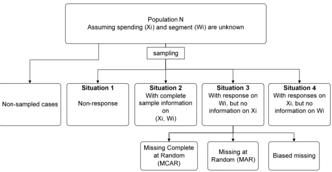
Adopting the segmentation approach admits two random variables, spending ( X ) and segmentation (W). We delimit our discussion and research design below to these two variables. For each sampled unit, four situations regarding the obtained data can be identified (Figure 1). The first situation represents the unit nonresponse, referring to units that refuse to participate, do not return the questionnaire or skip questions regarding spending and segment on the returned surveys. This leads to the unknown of X and W in the sampled unit. In contrast, situation 2 is that the case in which both X and W information is provided. Situations 3 and 4 reflect item nonresponse, representing cases that provide segmentation information but leave the spending questions blank, or the other way around. In this paper, the research scope includes only situations 2 and 3. Situation 4 will not be discussed at this time since it is less likely for respondents to skip the segmentation question but give out full spending profiles.

Using the terminology from Little and Rubin (2002), if the probability of nonresponse on spending (φ) is independent from the amount of spending (X), segment (W) or the survey design, the missing data are missing completely at random (MCAR). In this instance, the respondents are representative of the selected sample. If φ depends on segmentation but not on spending, the data are missing at random (MAR), for example, day visitors have a consistently lower response rate of spending than overnight visitors. Thus, the nonresponse can be modeled and the spending is adjusted based on the observed covariates (segment). If

φ depends on spending and cannot be completely explained by values of segmentation, this

results in biased missing. Under this circumstance, the nonresponse bias is non-ignorable but can not be fully accounted for.

Next, notation is introduced. Suppose there are m segments in a population. Let be a random sample from the population, where is the corresponding spending of the sample unit,

) , ,

(X_j W_j C_j j=1,_K,n X_j i

W_j = means that the individual comes from the

th

segment, and is a zero-one indicator representing whether the respondent provides spending information. Other symbols are

i C_j

i j

jW i X

E( = )=μ : the expected spending of the ith segment

2 ) (X_jW_j i _i

Var = =σ : the spending variance of the ith segment

i

j i P

W

P( = )= ; the proportion of the th

segment in the population i ) ( 1

∑

= = m i i i p

T μ : the average spending per unit of the population

1 = j

C : spending and segment are both observed for the jth unit, referred to as “complete case”

0 = j

C : spending is missing but segment is observed for the jth unit, referred to as “incomplete case”

C

n : Number of complete cases in the sample

I

n : Number of incomplete cases in the sample ) | 1 (C W i P _{j j} i = = =

γ : Probability of observing complete spending data in the ith

segment.

We estimate the average spending of each segment based on the complete observations ( ), and using the overall observations (

I n

I c n

n + ) to estimate the proportion of segment shares. Then, the estimated average spending is computed as Equation 3.

ated average spending (3)

Where

= average spending in the ith segment

= the sample pr

t where is

observed

= the sample size of the ith segment where is not

observed

icator function which is equal to 1 if the statement inside the

The variance computation formula for the weighted average spending when spending and

heorem 1

hat and are independent of each other within a segment, that is

∑

= = m i i i p T 1 ) ˆ ˆ ( ˆ _μ Estim

∑

= = = = n j j j j Ci i ₁X I(W i,C 1)/n , ˆ μ

oportion of the ith segment n n n pˆi =( C,i + I,i)/

∑

= = = n j j j i C I W n 1

, ( i,C =1) = the sample size of the i

th segmen X_j

∑

= = n j I ( j = j = i I W i C n 1 , , 0) Xj (.) I is the ind

parentheses is a true statement, and equal to 0 otherwise.

segment shares are stochastic is introduced below.

T Assume t X_j C_j j j j C W X ⊥ | , then σ wea / ) ˆ (T T

n − kly converges to standard normal in distribution.

can be consistently estimated by 2 σ ] ) ˆ ˆ ˆ 2 1 1 1 2 ( ) ˆ ˆ [( ˆ / ˆ ˆ 2

∑

2

∑

+ − = m i i i i m i= piσi γ = pμ

∑

= m i piμi σ (4) Where

) 1 /( ) ˆ )( 1 , ( ˆ 2 _, 1 = = − − =

∑

₌ Ci n j j j j i i I W i C X μ n σ ) /( ˆ_i =n_C,i n_C,i+n_I,i γ

The main assumption in Theorem 1 is that the missing pattern of spending (φ) of the individual case is assumed to be independent from the spending within each segment. In other words, the missing proportion remains constant across all sampled units in the same segment regardless of their high vs. low spending profile. This assumption is equal to the property of missing at random (MAR).

The 95% CI of T is computed as Tˆ±1.96×se(Tˆ) where I C m i i i m i i i i m i i i I C n n p p p n n T se + − + = + = _ˆ/

∑

= ˆ ˆ / ˆ [(

∑

= ˆ ˆ ) (

∑

= ˆ ˆ ) ] ) ( 2 1 1 2 1 2 γ μ μ σ σ ) ₍₅₎

The first component of equation 5,

I C i m i i i n n p +

∑

=1 ˆσˆ /γˆ 2

, represents the total variance

associated with spending within an individual segment. It can be rewritten as

∑

m₌ i i C i i n p 1 , 2 2 ˆ ˆ σ because ) ( _{, ,} , i I i C i C i n n n + =

γ . When tends to infinity, it indicates the recreation usages by

segments are fully recorded and the segment shares ( ) are deterministic. For a fixed

number of and infinite number of , I n i p C n nI

∑

₌ m i i C i i n p 1 , 2 2 ˆ ˆ σ will converge to

∑

= m i Ci i i n p 1 , 2 2 ˆ σ with probability one.

The second component of equation 5, ) ( ] ) ˆ ˆ ( ) ˆ ˆ [( ₁ 2 ₁ 2 I c m i i i m i i i n n p p + −

∑

∑

= μ = μ _{, represents the} variance associated with segment shares. An increase of incomplete cases ( ) will reduce the variance of segment shares, and subsequently the variance of average spending. When tends to infinity, the variance of

I n

I n

Tˆ reduces to the condition when pi (i=1,L,m) are known and the second component of Equation 5 will converge to zero.

4. SIMULATION

Four study designs for the segmentation approach are proposed in this paper, each involving different logics for handling complete cases ( ) and incomplete cases ( ). Simulation analysis is adopted to evaluate the accuracy and precision of the average spending estimator based on different study designs. In the simulation analysis, hypothetical data is first specified to represent the true population spending, variance and segmentation. For each design, ten thousand runs of simple random sampling are implemented. Simulated results for spending estimation are then compared to the true population value to establish the level of accuracy and precision of the estimator.

C

n n_I

4.1 Study designs

Four study designs are described in detail below.

Design 1

Conduct one wave of visitor surveys to collect spending and segmentation

information. Only complete cases ( ) are used in computing the average spending and segments. Incomplete cases on spending, if any, are excluded in the analysis. This scenario corresponds to the situation where the average spending is estimated without

C n

the segmentation approach because no additional information on segment shares is available.

Design 2

Conduct one wave of visitor surveys to collect spending and segmentation information. Calculate the average spending based on complete cases ( ), and compute segment shares based on the sum of complete cases ( ) and incomplete cases ( ). The proportion between complete and incomplete cases ( ) is determined by a given probability (

C n * C n I n n

φ). The number of incomplete case obtained is not

in direct control of researchers, which may vary case by case. Using this approach, the refusal rate by segment (φi) can be estimated.

Design 3

Conduct two waves of visitor surveys. One wave is to collect spending and segmentation information while the other wave of surveys is only to collect

segmentation information. The additional cases ( ) collected are determined by a ratio, pre-specified by researchers. In other words, the number of incomplete case obtained is in direct control of researchers. Calculate the average spending based on complete cases ( ), and compute segment shares based on the sum of complete cases ( ) and incomplete cases ( ). Using this approach, the refusal rate by segment ( I n C n C n nI i φ ) can be estimated. Design 4

Conduct one wave of visitor surveys to collect spending and segmentation

equivalent to infinite numbers of incomplete cases ( ). First use complete cases ( ) to compute the average spending by subgroup and then the weighted average is

computed based on given segment shares. This study design sets the basis for

precision comparison because segment shares do not introduce variation in this setting. I

n nC

4.2 Simulation process

A population with size of 100,000 is first generated and divided into four subgroups. The default spending average and variance for each subgroup are obtained from a visitor survey (Stynes & Sun, 2005b) to represent the actual spending patterns that have been observed. The actual spending is approximated to the gamma distribution, which is right-skewed and bounded at zero. Based on the default average spending and variance, probability density function of the gamma distribution is established for each segment, where the

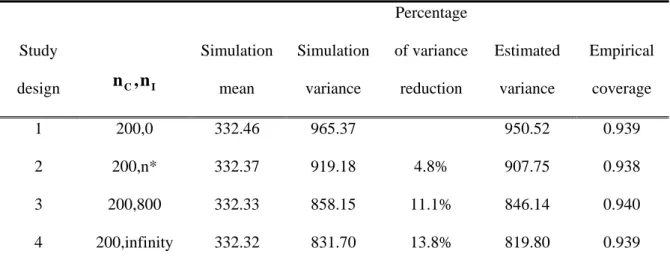
spending is generated for each unit. Respectively, the population size, spending average, and spending variance of segment 1 to 4 are (15000, 67.19, 8359), (5000, 134.85, 10217), (65000, 446.56, 243185) and (15000, 160.41, 13760) (Table 1). This gives a population mean of spending equal to $331.69, and population size of 100,000 party trips.

The probability of obtaining incomplete spending information (φ) is designed to have two sets of value, referred to as model 1 and model 2. For model 1, there is a one-third

probability (φ=0.33) that participants fail to provide average spending across all segments in the survey, as missing completely at random (MCAR). For model 2, the probability of obtaining incomplete spending information is assumed 1) to vary across four segments, in which φ equals 0.5, 0.2, 0.33 and 0.4, respectively, and 2) φ is independent from spending (MAR). Based on Leeworthy, et al (2001), Rylander, Propst, and McMurtry (1995) and

Stynes and Sun (2004), the average response rate of visitor spending by individual segment (φ_i) is different. This practical pattern leads to a reasonable specification of model 2.

For each study design, ten thousand runs of simple random sampling survey with a sample size of 200 complete cases and 400 complete cases are generated. Simulated results are compared against the true value to establish the accuracy and precision of the estimator, the average spending. Accuracy is compared based on the percentage difference between the estimator and the true value, while precision is based on the relative size of the variance.

Through ten thousand runs of simple random sampling, we can generate the following statistics for each study design.

ƒ Simulation mean: the sample average (spending) across 10,000 runs.

ƒ Simulation variance: the sample variance of the estimator across 10,000 runs. Based on the law of large numbers, simulated variance is approximated to the true variance.

ƒ Pct of variance reduction: the percentage of variance reduction when more information about the segment shares is added.

ƒ Estimated variance: variance computed based on Theorem 1 across 10,000 runs. ƒ Empirical coverage: the total number of runs in which the 95% CI of the sample

average spending covers the true average spending divided by ten thousand.

5. RESULT

With 200 complete cases in model 1, the simulated spending average is nearly identical (unbiased) to the true value, with difference less than 0.025% across four study designs (Table 2). The variance is reduced by approximately 5% and 11% when additional

and 800 incomplete data are included. The fourth design indicates that the variance could be reduced by up to 14% if the true proportion of each segment were known. This implies that, under the given parameters, spending accounts for more variation than segment shares.

*

The estimated variance through Theorem 1 is a slight under-estimate of the true variance, which leads to a smaller range of coverage. Subsequently, the empirical coverage is about 1% lower than 0.95.

When the sample size of complete cases is doubled to 400, the empirical power in this simulation is close to 95%, a better performance, and the simulation variance is reduced by approximately 50%. Although the spending of each individual case is generated from the gamma distribution, the distribution of the estimator is well approximated to the normal distribution when the sample size is 400.

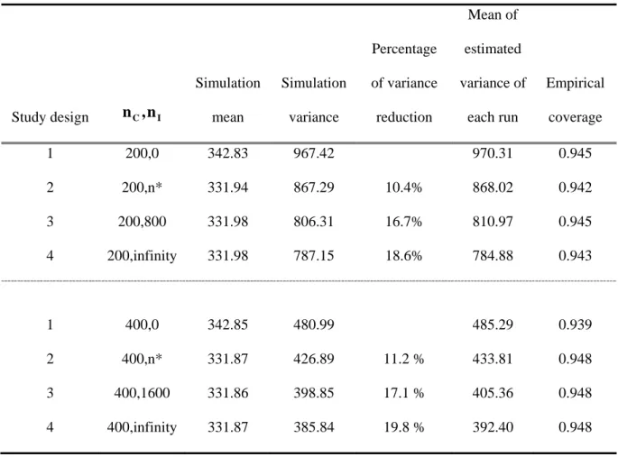
In model 2, we consider the case that the probability of missing information on the spending is different among segments as missing at random (MAR). The probability of refusal for giving out spending is 1/2, 1/5, 1/3 and 2/5, respectively. Under this setting, the simulation mean from the first study design is biased and over-estimated by 3.4% (Table 3). This is due to the fact that units of segment 1 and segment 4, the low-spenders, are under-represented in the sample, and the weighted average spending is biased toward groups with higher willingness to give complete spending information. No adjustment however can be implemented because additional information on covariate (segmentation) has not been considered in the analysis.

To correct for the problem of biased representation, additional information on

segment share through incomplete cases ( ) is needed. Study designs 2, 3 and 4 satisfy this condition and indicate that an unbiased result with a smaller sample variance is achieved. For example, there is about 17% variance reduction by including 800 additional incomplete data in the sampling process when =200. Comparing the results between Tables 2 and 3, it can be concluded that with more precisely-estimated segment shares, there is smaller variance for the average spending. However, the magnitude of variance reduction is not in direct

proportion to the number of incomplete cases ( ). The marginal variance reduction is more efficient for the first few incomplete cases than for those added at the end.

I n C n I n

6. STUDY DESGIN

Considering the reality of biased sampling and nonresponse patterns in general visitor expenditure surveys, inclusion of incomplete cases in the analysis corrects the segment share biases and reduces the sampling variance of the weighted average spending. Thus, inclusion of incomplete cases ( ) provides a better property of precision and accuracy on the spending estimation, which gives a support for Stynes and White’s claim for the segmentation

approach (1999; 2006). In the following, we provide further discussion on the study design, the selection of segmenting variables, and the decision on the ratio between and .

I n

I

n n_C

6.1 Study design

A typical study design in expenditure studies includes only cases with complete information on spending, as the study design 1 in our simulation. When faced with item nonresponse on expenditure, technical reports may suggest to replace the missing value with the overall sample average or “exclude records that provide no spending information as unusable”2 (Research Resolutions & Consulting Ltd, 2005, p. 6). Under this procedure, the estimator is unbiased only when the condition of missing completely at random (MCAR) is satisfied. However, this assumption is generally invalid, and excluding cases with item nonresponse will lead to a biased spending average. To correct this problem, expenditure surveys should incorporate other observed variables as the segment covariate to model the nonresponse mechanism of visitor spending.

The recommended study design conducts additional interviews to obtain responses of segments (referred to as short surveys) in addition to the regular visitor surveys (referred to as long surveys), as study design 3. This additional step involves an on-site exit survey with one or two questions to obtain the segment data. It generally takes only one or two minutes to

complete, which is cost, time and labor efficient. Due to the cost-efficient nature, a greater number of short surveys can be generated with a limited budget. Most importantly, it is more feasible to apportion samples throughout the longer study period (e.g., a year) to account for seasonal differences of user types, as well as cover a broader geographic area to capture activity differences among resource usages. By implementing this strategy, the representation of user groups in the sample to the study population can be enhanced accordingly. Secondly, due to the time-efficient manner and short questionnaire, respondent burden is reduced and a higher response rate from recreation participants on-site can be expected (Groves, 1989). This subsequently reduces the non-response bias and omission bias because these biases tend to amplify as the complexity of questionnaire expands and the lapse of time between the event and the interview increases.

Short on-site surveys can also be labor-efficient from the implementation perspective. Gathering of short-surveys can be assisted by the gate keeper of the recreational facilities or friends (volunteers) of the association, and becomes a routine task for the staff. For example, every 10th travel party can be briefly detained at the entrance gate to inquire their choices of lodging types in the region (assuming lodging is the segmenting variable) while their ticket is being collected. Although this alternative has the disadvantage of overly representing groups with higher re-entry rates, this drawback can be corrected by weighting the cases inversely proportional to the re-entry rate.

6.2 Segmenting variable

After knowing the preferred study design, the next question is how to choose the appropriate variable to segment the study population. Tkaczynski, Rundle-Thiele and Beaumont (2009) reviewed 115 tourism segmentation studies and indicated that there are numerous alternatives, ranging from demographic, behavioral, psychographic to geographic segmentation variables. For example, accommodation, recreation activity type, travel purpose,

and country of residence are the frequently adopted variables in recreational studies. There is no definitive answer regarding which variable is the most appropriate in a visitor expenditure survey as this may vary case by case, but three criteria are offered.

The first criterion suggested is to find the key factor that can efficiently differentiate spending patterns by user groups, reducing the spending variance within individual group ( ). In other words, a good classification should allow units within the same segment to have similar travel preferences and expenditure level. Lodging type, length of stay,

transportation mode and travel purposes are generally more effective in differentiating user consumption patterns by groups. Stynes (1999) recommended distinguishing user groups by their lodging types and distance from home to the destination, including day trips from the local region, day trips from outside the area, overnight visitors staying at hotels, overnight visitors staying at campgrounds, and overnight visitors staying at seasonal homes or visiting friends and relatives (VFR), respectively. This recommendation is based on the fact that lodging expenses account for the majority of trip expenses. Control of lodging type reduces the spending variance within the same segment.

2 i

σ

The second criterion is to seek out a condition where the missing behavior is independent from the spending level within each segment. A good segment variable exists when the behavior of giving incomplete information, not returning questionnaires, or implying no willingness to participate in a long survey is highly consistent and independent from the spending in the same sub-group. Based on Rylander et al.,(1995), local day visitors versus non-local overnight visitors is the basic distinction that can be adopted, as the former have a higher propensity not to give spending information. If this criterion is followed, the key assumption in Theorem 1, that the missing propensity is independent from the spending level within each segment (Xj ⊥Cj |Wj), will be valid to a greater extent.

Some marketing studies may use travel expenditure as the segmenting variable to understand the user characteristics associated with high/low spending patterns so that tourism

policies can be designed accordingly (Koc & Altinay, 2007; Laesser & Crouch, 2006; Mok & Iverson, 2000). From the perspective of estimating total expenditure by segments, using the high/low spending as a segmenting variable is not recommended because no other observed variable is adopted to adjust the possible nonresponse and biased sampling associated with spending. In addition, the use of a short survey recommended in this paper is not feasible since the segmentation is based on spending itself. This situation would then create “non-ignorable nonresponse” bias on the estimator.

The final criteria for choosing the segmenting variable is giving priority to those that are easily observable without causing too much burden on respondents in terms of time, effort or personal privacy. For example, lodging type and personal income are two key factors in determining trip expenditure. Income level, however, is harder to obtain onsite and may subject to false response. On the contrary, visitors are much more willing to give their lodging choices, which serves as a better segmenting variable than income.

For future research, a Meta analysis in reviewing empirical studies on segmentation and visitor spending will be helpful to reveal variables that satisfy the following conditions. First, this variable must influence expenditure pattern among recreation users so that

spending variance can be reduced within subgroup. Second, it must reflect consistent

response propensity and be independent from the spending level within the same sub-group. Cross referencing these two pools can provide the appropriate candidates as the segmenting variables in a spending survey.

6.3 Number of incomplete cases

The last component of the survey design is to consider how many additional short surveys are required or how to determine the number of long versus short surveys based on a fixed budget. Answers to this question depend on several factors simultaneously. First we

need to understand the effect of sample size, differentiating by and , on the overall variance level.

C

n n_I

In model 1, we have assumed missing completely at random (MCAR), so that

i I C i C i I i C i C i p n n n n n n ) ( , , , , + ≈ + ≈

γ and nC,i ≈nC*pi _. Therefore, the variance of weighted average

spending can be rewritten as

) ( ] ) ( ) [( ) ( ] ) ( ) [( ) ˆ ( 2 1 1 2 1 2 2 1 1 2 1 , 2 2 I c m i i i m i i i C m i i i I c m i i i m i i i m i i C i i n n p p n p n n p p n p T Var + − + ≈ + − + ≈

∑

∑

∑

∑

∑

∑

= = = = = = μ μ σ μ μ σ (6)

From equation 6, we can infer that when the sample size of complete cases on

spending ( ) is doubled, while holding all else constant, the variance of average spending is reduced by roughly 50%, or vice versa. The exact value will depend on the number of

incomplete cases and the variance associated with segment shares. Also, if the sample size on the complete cases is fixed (e.g., 400), more samples ( ) are allocated to the segment with a larger spending variation would reduce the overall variance to a greater extent because

would decrease. C n ( 1I W i C n _, ) 1 /( ) ˆ )( 1 , ˆ =

∑

n₌ = = − 2 _C,i − j j j j i i i C X μ n σ

On the contrary, holding complete cases and other parameters constant, the addition of short surveys will not reduce the estimator variance as efficiently as the long surveys do. This is because a short survey ( ) influences only the precision of segment shares, the second component of equation 6. By holding all else constant, the level of variation (

I n

Tˆ ) with regards to the short survey converges at a rate of (n_I−1) with probability one (equation 7).

Variance (Tˆ ) ≈ I n b a k + + (7)

By holding p_i,u_i,n_c,σ_iconstant, we can treat a,b,k>0and as constant

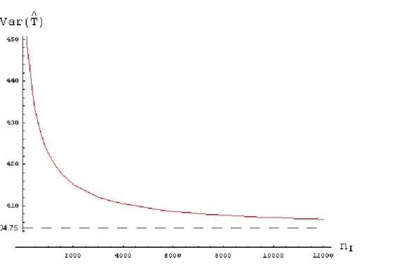
Using model 1 with complete case ( ) of 400 as an example, we plot the relationship between the sample variance and the number of incomplete cases ( ) in Figure 2. When increases from zero to 1000, 2000, and 3000, the variance reduces to 423, 415, and 412, respectively. As the number of continues to expand, the variance gradually approaches 404.75. A convex plot in figure 2 clearly indicates that the marginal error reduction rate is much higher in the early stage and becomes inefficiently lower as expands. Based on the specified parameters in model 1, the best combination of versus is approximately 1: 5, since beyond this point, the contribution of on variance reduction is negligible. The

addition of short surveys therefore should not be unlimited. To determine the appropriate sample size of , researchers should take into consideration of survey cost per , the expected variance level of spending, and the marginal error reduction rate, simultaneously.

C n I n I n I n n I n I n C n _I I n nI

Besides marginal variance reduction rate, the maximum level of error reduction in adding short surveys is another key factor to be considered. In model 1, the spending variance can be reduced by 14% if the segment is deterministic while the variance in model 2 can be reduced up to 20% (Table 2 and 3). To understand the cause of differences, we compare the spending variances when is given at a finite number versus is infinity (Equation 8). When tends to infinity, the segment shares are determined and no variation is introduced, which sets the basis for precision comparison.

I

n n_I

I n

Comparison of estimator variance

= ⎥ ⎥ ⎦ ⎤ ⎢ ⎢ ⎣ ⎡ + ⎥ ⎥ ⎦ ⎤ ⎢ ⎢ ⎣ ⎡ + − +

∑

∑

∑

∑

= = = = I C i m i i i I C m i i i m i i i i m i i i n n P n n p p Pσ γ μ μ σ /γ / ] ) ( ) [( / 1 2 2 1 1 2 1 2 =

∑

∑

∑

= = = + − + _m i i i I C C m i m i i i i i p n n n p p 1 2 1 2 1 2 * ) ( * ] ) ( [ 1 σ μ μ (8)

Plotting in the default parameters from Table 1, this ratio from equation 8 is equal to

( I C C n n n + +0.15695*

1 ). In other words, in model 1, the estimator variance without obtaining

additional information on segment shares ( = 0) is 1.157 times the estimator variance when segment shares are known. If is equal to , the estimator variance is 1.078 times that w segment shares are deterministic. The level of variance reduction is greatly influenced by the

segment share variance,

I n C n I n hen

∑

∑

∑

= = i1p [

arger this component is, the more

worthwhile to make extra effort to obtain additional information through n_I. = − m i i i i i p 1 2 2 ] ) ( σ μ μ . The l i m i pi 2 1 m

Therefore, for model 1, the maximum level of variance reduction from segmentation will depend on the relative segment shares across groups ( ), the average spending by each

group (

i p

i

μ ), number of complete cases ( ) and spending variation within groups ( ). For

model 2, when the response rate is different across groups3, the variance reduction level would then depend on and the probability of giving full spending information,

C n σi2 2 , , , _{i c i} i n p μ σ i γ .

Based on the above discussion, it is recommended to design expenditure surveys by implementing two waves of data gathering, one for collecting the spending and segment information and the other wave for collecting segmentation only. If the expenditure study is aimed for a longer period, the first step is to get a rough idea for the level of segment shares,

average spending, and variance by user groups in the study population through long surveys ( ). Obtaining such information would then help researchers to calibrate the appropriate number of short surveys ( ) by taking into consideration the associated variance reduction level and operating costs per collected survey.

C n

I n

7. CONCLUSION

Adopting the segmentation strategy to estimate total visitor consumption has several advantages in terms of policy management, evaluation, and sampling design. However, this approach requires two sets of information – average spending per segment as well as segment share so that total visitation can be apportioned to each subgroup. Both variables generally rely on visitor surveys for estimation. To gather this information, Stynes (1999) and Stynes and White (2006) recommend conducting a short survey to investigate visitor segments in addition to regular visitor surveys (full survey) on spending. This paper expands their discussion further in two directions. First, a statistical formula is provided to compute the estimator variance by taking into account the stochastic nature of spending and segment shares. This formula provides a convenient step to understand the variance level introduced by segmentation. Using simulation analysis, we demonstrate that acquiring more information on the segment share helps to reduce the variance of the weighted average spending so that better precision is attained. Secondly, the addition of segment information will not reduce the estimator variance in a linear pattern so that there is no need to generate an excessive number of short surveys. The key is to allocate the short surveys to be representative of the time and location of recreational usage across the study region. Optimization analysis can then be performed based on expected level of variance reduction, subject to constraint of time, manpower, and survey materials, to reach a balance between data quality and operating cost between full and short surveys.

Acknowledgements: Constructive comments from Dr. Ariel Rodriguez at Arizona State University and anonymous referees are highly appreciated. Financial support from the Taiwan National Science Council under NSC 98-2410-H-390 -029 -SS2 is acknowledged.

8. REFERENCE

Baird, B. F. (1989). Managerial decisions under uncertainty: An introduction to the analysis of decision making. New York: Wiley-Interscience.

Breen, H., Bull, A., & Walo, M. (2001). A comparison of survey methods to estimate visitor expenditure at a local event. Tourism Management, 22, 473-479.

Diaz-Perez, F. M., Bethencourt-Cejas, M., & Alvarez-Gonzalez, J. A. (2005). The segmentation of canary island tourism markets by expenditure: Implications for tourism policy. Tourism Management, 26(6), 961-964.

Efron, B. (1979). Bootstrap methods: Another look at the Jackknife. Annals of Statistics, 7(1), 1-26.

English, D. B. K. (2000a). Calculating confidence intervals for regional economic impacts of recreation by bootstrapping visitor expenditure. Journal of Regional Science, 40(3), 523-539.

English, D. B. K. (2000b). A simple procedure for generating confidence intervals in tourist spending profiles and resulting economic impacts. The Journal of Regional Analysis & Planning, 30(1), 59-74.

Fleming, W. R., & Toepper, L. (1990). Economic impact studies: Relating the positive and negative impacts to tourism development. Journal of Travel Research, 29(1), 35-42. Frechtling, D. C. (2006). An assessment of visitor expenditure methods and models. Journal

of Travel Research, 45(1), 26-35.

Groves, R. M. (1989). Survey errors and survey costs. New York: John Wiley & Sons, Inc. Hays, W. L. (1994). Statistics (5th ed.). Belmont, CA: Wadsworth/ Thomson Learning. Kish, L. (1995). Survey sampling. New York: John Wiley & Sons, Inc.

Koc, E., & Altinay, G. (2007). An analysis of seasonality in monthly per person tourist spending in Turkish inbound tourism from a market segmentation perspective. Tourism Management, 28(1), 227-237.

Kotler, P. (1980). Principles of marketing (1st ed.). New Jersey: Prentice-Hall.

Laesser, C., & Crouch, G. I. (2006). Segmenting markets by travel expenditure patterns: The case of international visitors to Australia. Journal of Travel Research, 44(4), 397-406. Lai, S. Z., & Wong, K. F. (2008). Computation of joint confidence intervals for the weighted

average. Kaohsiung, Taiwan: National University of Kaohsiung.

Leeworthy, V. R., Wiley, P. C., English, D. B. K., & Kriesel, W. (2001). Correcting response bias in tourist spending surveys. Annals of Tourism Research, 28(1), 83-97.

.htm

Little, R. J. A., & Rubin, D. B. (2002). Statistical analysis with missing data (2nd ed.). New Jersey: Wiley-Interscience.

Lohr, S. L. (1999). Sampling: Design and analysis. Pacific Grove, CA: Brooks/Cole Publishing Company.

Loomis, J. (2007). Correcting for on-site visitor sampling bias when estimating the regional economic effects of tourism. Tourism Economics, 13(1), 41-47.

Mok, C., & Iverson, T. J. (2000). Expenditure-based segmentation: Taiwanese tourists to Guan. Tourism Management, 21(3), 299-305.

Orens, A., & Seidl, A. (2004). Winter tourism and land development in Gunnison, Colorado. Fort Collins, CO: Department of Agricultural and Resource Economics, Colorado State University.

Ormer, C. V., Littlejohn, M., & Gramann, J. H. (2001). Olympic National Park visitor study: University of Idaho.

Pannell, D. J. (1997). Sensitivity analysis of normative economic models: Theoretical framework and practical strategies. Agricultural economics, 16(2), 139-152. Pol, A. P., Pascual, M. B., & Vazquez, P. C. (2006). Robust estimators and bootstrap

confidence intervals applied to tourism spending. Tourism Management, 27(1), 42-50. Research Resolutions & Consulting Ltd. (2005). Guidelines for measuring on-site spending at

gated and ungated events and festivals Appendices I - IV. Retrieved from http://www.rpts.tamu.edu/impacts/page3_Gated

Rylander, R. G., Propst, D. B., & McMurtry, T. R. (1995). Nonresponse and recall biases in a survey of traveler spending. 33(4), 39-45.

Simmons, T., & Gramann, J. H. (2001). Badlands National Park visitor study: University of Idaho.

Smith, S. L. J. (2000). New developments in measuring tourism as an area of economic activity. In W.C.Gartner & D. W. Lime (Eds.), Trends in outdoor recreation, leisure and tourism (pp. 225-234). New York: CAB International.

Stynes, D. J. (1999). Guidelines for measuring visitor spending. Retrieved from https://www.msu.edu/course/prr/840/econimpact/pdf/ecimpvol3.pdf

Stynes, D. J., & Sun, Y.-Y. (2003). Economic impacts of National Park visitor spending on gateway communities, systemwide estimates for 2001. East Lansing, MI: Department of Park, Recreation and Tourism Resources, Michigan State University.

Stynes, D. J., & Sun, Y.-Y. (2004). Economic impacts of national heritage area visitor spending; Summary results from seven national heritage area visitor surveys. East

Lansing, MI: Department of Community, Agriculture, Recreation and Resource Studies, Michigan State University.

Stynes, D. J., & Sun, Y.-Y. (2005a). Economic impacts of visitors to Grand Canyon National Park, 2003. East Lansing, MI: Department of Park, Recreation and Tourism

Resources, Michigan State University.

Stynes, D. J., & Sun, Y.-Y. (2005b). Impacts of visitor spending on the local economy: Arches National Park 2003. East Lansing, MI: Department of Park, Recreation and Tourism Resources, Michigan State University.

Stynes, D. J., & White, E. M. (2006). Reflections on measuring recreation and travel spending. Journal of Travel Research, 45(1), 8-16.

Sun, Y.-Y., & Stynes, D. J. (2005). Survey biases from three National Park Service visitor studies. Paper presented at the Annual Travel & Tourism Research Association Conference, New Orleans, Louisiana, USA.

Tkaczynski, A., Rundle-Thiele, S. R., & Beaumont, N. (2009). Segmentation: A tourism stakeholder view. Tourism Management, 30(2), 169-175.

Weiler, S., Loomis, J., Richardson, R., & Shwiff, S. (2002). Driving regional economic models with a statistical model: Hypothesis testing for economic impact analysis. The Review of Regional Studies, 32(1), 97-111.

Wilton, J. J., & Nickerson, N. P. (2006). Collecting and using visitor spending data. Journal of Travel Research, 45(1), 17-25.

Wood, D., & Hughes, M. (2006). Tourism accommodation and economic contribution on the Ningaloo Coast of Western Australia. Tourism and Hospitality Planning &

Development, 3, 77-88.

World Tourism Organization. (1995). Collection of tourism expenditure statistics. Madrid: World Tourism Organization.

Table 1 Parameters for simulation

Segments

Population

Prob. of obtaining incomplete spending information (φ)

Mean Variance Size Model 1 Model 2

Group 1 67.19 8359 15,000 0.33 0.50 Group 2 134.85 10217 5,000 0.33 0.20 Group 3 446.56 243185 65,000 0.33 0.33 Group 4 160.41 13760 15,000 0.33 0.40 Total 100,000 Weighted average 331.69

Table 2 Summary results of model 1 with 200 and 400 complete data Study design nC,nI Simulation mean Simulation variance Percentage of variance reduction Estimated variance Empirical coverage 1 200,0 332.46 965.37 950.52 0.939 2 200,n* 332.37 919.18 4.8% 907.75 0.938 3 200,800 332.33 858.15 11.1% 846.14 0.940 4 200,infinity 332.32 831.70 13.8% 819.80 0.939 1 400,0 331.81 470.85 471.73 0.948 2 400,n* 331.83 450.39 4.3% 450.64 0.949 3 400,1600 331.77 418.46 11.1% 420.40 0.948 4 400,infinity 331.72 405.56 13.9% 407.40 0.947

Table 3. The summary results of model 2 with 200, 400 complete data Study design nC,nI Simulation mean Simulation variance Percentage of variance reduction Mean of estimated variance of each run Empirical coverage 1 200,0 342.83 967.42 970.31 0.945 2 200,n* 331.94 867.29 10.4% 868.02 0.942 3 200,800 331.98 806.31 16.7% 810.97 0.945 4 200,infinity 331.98 787.15 18.6% 784.88 0.943 1 400,0 342.85 480.99 485.29 0.939 2 400,n* 331.87 426.89 11.2 % 433.81 0.948 3 400,1600 331.86 398.85 17.1 % 405.36 0.948 4 400,infinity 331.87 385.84 19.8 % 392.40 0.948

Figure 2. The relationship between var(Tˆ ) and number of incomplete cases (n_I)

Footnote

1

For detailed sampling methods and sample size, please refer to Ormer, Littlejohn, and Gramann (2001) and Simmons and Gramann (2001).

2

This report (Research Resolutions & Consulting Ltd, 2005) provides a precaution that “excluding cases with no spending information” should be considered only if the target number of completions per cell is achieved. However, increasing sample size without targeting nonresponse does not reduce nonresponse bias (Lohr, 1999).

3

For model 2, it is more difficult to analyze the relationship between estimator variance and number of income cases (n_I), because the assumption of n_C,i ≈n_C*p_idoes not hold due to different response rate of full survey by individual segment (γi). Therefore, it must be analyzed case by case. In the example of model 2 with = 200, due to large sample theorem, C n 32 . 313 6 . 0 * 15 . 0 3 / 2 * 65 . 0 8 . 0 * 05 . 0 5 . 0 * 15 . 0 200 _≈ + + + ≈ n so that nC,i ≈313.32*pi*γi. and 20 . 28 6 . 0 * 15 . 0 * 32 . 313 45 . 136 67 . 0 * 65 . 0 * 32 . 313 53 . 12 8 . 0 * 05 . 0 * 32 . 313 50 . 23 5 . 0 * 15 . 0 * 32 . 313 4 , 3 , 2 , 1 , ≈ ≈ ≈ ≈ ≈ ≈ ≈ ≈ C C C C n n n n

This implies that

) ( ) ( ) ˆ ( 1 2 1 2 1 , 2 2 I C m i m i i i i i m i i C i i n n p p n p T Var + − + ≈

∑

∑

=

∑

= = μ μ σ ) 200 ( 25410 78 . 777 I n + + ≈ . The

estimator variance without obtaining additional information on segment shares ( = 0) is 1.163 times the estimator variance when segment shares are known. If is equal to , the estimator variance is 1.082 times that when segment shares are deterministic.

I n

I

Appendix

Theorem 1 can be discussed in two parts and the proof is provided below.

Theorem 1.1：Suppose (Xj,Wj,Cj), j =1,2,K,nbe independent, identically distributed random vectors with E(X_jW_j =i)=μ_i,Var(X_jW_j =i)=σ_i2 and P(C_j =1W_j =i)=γ_i >0, in which (I(W_j =1),_K,I(W_j =m))~Multinormial(1,p₁,_K,p_m)andC_j =I(X_jis observed . )

Let , ) ( ˆ , ˆ , 1 i C n j j j j i i i N X i W I C n N p

∑

= = = = μ 1 ) ˆ )( ( ˆ , 1 2 2 − − = =

∑

= i C n j j j j i i N X i W I C μ σ and , ˆ ˆ ˆ 1

∑

= = m i i i n p T μ where NC,i =

∑

n_j=1CjI(Wj =i) and =

∑

₌ = n j j i I W i N ₁ ( ).

Assume further thatCj ⊥XjWj , then

) 1 , 0 ( ˆ N T T n n − → σ in distribution, where

∑

= = m i pi i T 1 μ and 2 1 2 1 2 2 1 T p p m i i i m i i i i − + =

∑

₌ σ

∑

₌ μ γ σ .

In addition, σ2 can be consistently estimated by ₁ 2 ₁ 2 2 , 2 _ˆ ˆ ˆ ˆ ˆ m _n i i i m i i i i C i n p p T N N S =

∑

₌ σ +

∑

₌ μ − .

Theorem 1.2 ：Under the assumptions in Theorem 1.1, let W_j, j =n+1,_K,n+n_I be independent, identically distributed random variables which has the same

distribution as W1. Also,Wj, j =n+1,K,n+nI and (Xj,Wj,Cj), j=1, 2, are independent. Let n , K I i I i n i n n N N p I + + = , , ˆ , =

∑

m₌ and i in i n n I p I T 1 , , ˆ ˆ ˆ _μ 2 , 1 2 , 2 , ( ˆ ˆ ˆ 1 I I I nn m i in i I n n p T n n S ₁ , 2+ − , , ˆ ˆ I m i in i i C i I i p N N N + + =

∑

₌ σ

∑

₌ μ , where =

∑

n+₌n₊I = n j j i I I W i N , ₁ ( ).

Then given ε >0 and x∈ , there is an N∈ such that

ε < ≤ − ∪ Ν ∈ | ˆ | sup , , } 0 { x S T T I I I n n n n n

whenevern≥N.

The proof of Theorem 1.1 is similar as the proof of Theorem 1.2. Thus, we give only the proof of Theorem 1.2 here.

Proof：Let 1, 2, be independent, identically distributed 2m-dimensional random vectors each with mean

= j

Yj, K,n Y

μ and covariance matrix ∑ , where

⎟ ⎟ ⎟ ⎟ ⎟ ⎟ ⎟ ⎟ ⎠ ⎞ ⎜ ⎜ ⎜ ⎜ ⎜ ⎜ ⎜ ⎜ ⎝ ⎛ = ⎟ ⎟ ⎟ ⎟ ⎟ ⎟ ⎟ ⎟ ⎠ ⎞ ⎜ ⎜ ⎜ ⎜ ⎜ ⎜ ⎜ ⎜ ⎝ ⎛ = = − = − = = m m Y m j j m j j j j j j j p p m W I W I X m W I C X W I C Y μ μ μ μ μ μ μ M M M M 1 1 1 1 0 0 , ) ( ) 1 ( ) )( ( ) )( 1 ( .

By Central Limit Theorem,

) , 0 ( ] 0 0 ) ˆ ( ) ˆ ( [ 1 1 1 1 , 1 1 1 , ∑ → ⎟ ⎟ ⎟ ⎟ ⎟ ⎟ ⎟ ⎟ ⎠ ⎞ ⎜ ⎜ ⎜ ⎜ ⎜ ⎜ ⎜ ⎜ ⎝ ⎛ − ⎟ ⎟ ⎟ ⎟ ⎟ ⎟ ⎟ ⎟ ⎟ ⎟ ⎟ ⎟ ⎟ ⎠ ⎞ ⎜ ⎜ ⎜ ⎜ ⎜ ⎜ ⎜ ⎜ ⎜ ⎜ ⎜ ⎜ ⎜ ⎝ ⎛ − − N p p n N n N n N n N n m m m m m m m C C μ μ μ μ μ μ μ μ M M M M in distribution. Suppose, L n n n n I n→∞ + _{( )} =

lim . IfL<1, by Central Limit Theorem again, we have

) , 0 ( ] ) ( ) ( [ ) ( * 1 1 , 1 1 , ∑ → ⎟ ⎟ ⎟ ⎠ ⎞ ⎜ ⎜ ⎜ ⎝ ⎛ − ⎟ ⎟ ⎟ ⎟ ⎟ ⎟ ⎠ ⎞ ⎜ ⎜ ⎜ ⎜ ⎜ ⎜ ⎝ ⎛ N p p n n N n n N n n m m m I m I I I I

μ

μ

μ

μ

M

M in distribution, where is the

covariance matrix of * ∑ ). ) ( , , ) 1 ( (I Wj = μ1 K I Wj =m μm

IfL=1, then for every ε >0 , by Chebychev’s inequality,

0

))

(

(

)

1

(

)

(

)

)

)

(

(

)

(

)

(

)

(

(

, _{2 2}

→

+

−

≤

≥

−

+

n

n

n

p

p

n

nn

p

n

n

N

n

n

n

n

n

n

nn

P

I i i I i I i I I I I

ε

ε

_{as n→∞, i=1,K,m.}