熵應用於交通資料融合之研究

全文

(1)國立交通大學運輸科技與管理學系碩士論文 ! !. ⧅ ᐷ σ ٜ ϛ ఞ ྆ ी Ꭻ Ќ ˿ ࠣ ա! The Application of Entropy on Data Fusion of Traffic Information ! ! ! ! ! 研究生：吳欣潔指導教授：王晉元. 中華民國九十三年六月.

(2) 熵應用於交通資料融合之研究 The Application of Entropy on Data Fusion of Traffic Information 研究生：吳欣潔. Student：Hsin-Chieh Wu. 指導教授：王晉元. Advisor：Jin-Yuan Wang 國立交通大學運輸科技與管理學系碩士論文. A Thesis Submitted to Department of Transportation Technology and Management College of Management National Chiao Tung University In Partial Fulfillment of the Requirements for the Degree of Master of Engineering In Transportation Technology and Management June 2004 Hsinchu, Taiwan, Republic of China. 中華民國九十三年六月.

(3) 熵應用於交通資料融合之研究學生 : 吳欣潔. 指導教授 : 王晉元國立交通大學運輸科技管理學系碩士班. 摘. 要. 在許多智慧型運輸系統(ITS)的應用中，即時資訊的需求越來越高，為了能提供正確可靠的資訊，ITS 應用所提供的資訊必須持續更新，意謂著資料收集與處理過程必須持續進行。然而，由於資料來源(如偵測器、探針車等)有偵測範圍的限制且資料量通常不大，易造成資料的可靠度降低。藉著資料融合的過程，可以改善以上問題。資料融合的觀念始於 1980 年左右，而在近年才有許多資料融合方法的發展與應用。回顧在 ITS 領域中相關的資料融合研究，主要可以將這些技術分成三個層級，其中，層級二的資料融合技術能夠提供由原始資料而來的推論以及更完備資訊，因此本研究的目的是在發展層級二的資料融合模式。熵值的應用是由 C. Shannon 在 1948 年所提出，最早被用於“信息理論＂，之後，熵值被廣泛地應用於量測不確定性，本模式中，提出了資料分級的方式使得熵值可以應用在量測各資料來源的不確定性。而由於熵值所代表的含意為不確定性，模式也更進一步推導權重與熵值的關係，給予每個資料來源最佳的權重。為了測試模式的適用性，我們設計了一連串的實際測試。而在資料收集不易以及資料量不大的情況下，我們亦使用模擬的資料來進行測試。測試結果證實本研究所提出的資料融合方法在實務上具有可行性。. 關鍵字：旅行者資訊、資料融合、智慧型運輸系統、先進旅行者資訊系統、熵.

(4) The Application of Entropy on Data Fusion of Traffic Information Student : Hsin-Chieh Wu. Advisor : Jin-Yuan Wang. Department of Transportation Technology and Management National Chiao Tung University. Abstract Real-time travel information is becoming increasingly important in many intelligent transportation system (ITS) applications. In order to provide reliable information to the users, traffic information in all the ITS applications should be comprehensive and continually updated. It means that a continuous real-time data collection and processing effort is essential to provide the required information. However, data sometimes is not reliable since every source has a certain detecting range and the data volume is often small. These problems can be addressed by data fusion process. Data fusion technology started in the late 1980s and many data fusion approaches had been developed and applied in recent years. In reviewing data fusion techniques in ITS field, the techniques can be divided into three levels. In our model, we propose data fusion techniques focus on the level two since level two data fusion provides a higher level of inference and delivers additional interpretive meaning suggested from the raw data. Entropy is a concept proposed by C. Shannon in the 1948 and is used in “ Information Theory” first. Shannon’s entropy function has been used extensively as a measure of uncertainty. We propose a classifying approach so that we can cite the entropy to measure the uncertainty of the collected traffic data. Since entropy represents the uncertainty, we form an optimal weight scheme and use entropy to derive the weight of each sensor. We perform a series of tests for model evaluation purpose. Since collecting real data is hard in practice and the volume of real data is often small, we also use simulated data to test our model. The testing results show that our proposed entropy data fusion technique is suitable in practice.. Keyword: Traveler Information, Data Fusion, ITS, ATIS, Entropy.

(5) 誌. 謝. 本研究得以順利完成，首先要感謝的就是王老師。從研一開始就感受到老師的功力，總覺得老師想都不用想就可以解決我們抓破頭也想不透的問題，真是太厲害了！而老師除了要指導我們的論文內容，還要讓我們殘破不堪的英文能夠總合成一篇文章，我想，老師真的很辛苦，在這裡向老師致上最高的謝意。另外，也謝謝老師貼心的提供 Lab 多次出遊，讓大家的感情更好、生活更充實。感謝成功大學交管系魏健宏教授以及交通部運輸研究所吳玉珍組長在論文口試過程中給予相當多寶貴的意見及指導，使本論文更臻完備。兩年的碩士生涯就要結束了，回顧這兩年來，大部分的時間都是待在 Lab 裡。感謝大師兄時時給我研究上的指導(包括保齡球)；感謝紀舜、東凌學長在計畫案、論文上的幫忙；奈特、阿信、猴子、嘉龍這幾個一起同甘共苦的好兄弟，我想我們都不會忘記每次咪挺前抽牌比大小以及戰戰兢兢地敲老師辦公室的門的情景；感謝小名、家盛、穹林、駿逸，讓我們知道英文要早點開始寫(^^||| 當然還有計畫、課業的討論)；感謝怡君、彥祐，雖然你們不常在 Lab，可是需要幫忙的時候你們都會及時出現，還有齁齁，學到你萬分之一罵髒話的功力，我以後在社會上應該不會罵輸人家；感謝衍儒幫我們處理繁瑣的工作費之外，還要幫忙辦出遊；感謝嘉英、信翔、思文，使我們計畫案的 loading 少了好多。感謝室友 jas、wena、huiyu 多年的幫忙與照顧，除此之外，還有許多大學、研究所的好朋友，、韻璇、起豪、紀百、thomas、則言、梅子、elephant、大中、小宇、耀楨、苑綾、大哥、阿貴、小渣、佳琴…，和你們的相處都充實了我的研究生生活。最後要感謝的是一直在背後默默支持我的家人，謝謝你們提供我一切資源，讓我在求學的過程中一路順利，沒有後顧之憂。也謝謝你們包容與體諒我有時因為課業而缺席家裡的活動。謝謝各位在這段日子裡參與我的生活，在此與大家一同分享論文完成的喜悅，誠心的感謝大家！. 吳欣潔新竹交大 2004/7/5.

(6) Content Content ...................................................................................................................I Figure List ............................................................................................................ II Table List ............................................................................................................. III Chapter 1 Introduction .......................................................................................... 1 1.1 Motivation ................................................................................................ 1 1.2 Objectives ................................................................................................. 2 1.3 Scope ........................................................................................................ 2 1.4 Study Flowchart ....................................................................................... 4 Chapter 2 Literature Review ................................................................................. 6 2.1 Review of Data Fusion Developments..................................................... 6 2.1.1 Introduction to Data Fusion............................................................ 6 2.1.2 Benefits of Data Fusion.................................................................. 8 2.2 Review of Level two Data Fusion Algorithms......................................... 8 2.2.1 The Team Consensus Approach ..................................................... 8 2.2.2 Introduction to Entropy ................................................................ 10 Chapter 3 Model Building................................................................................... 12 3.1 The Concept of Data Classifying ........................................................... 13 3.2 The Concept of Entropy Calculating...................................................... 15 3.3 The optimal weighting scheme .............................................................. 16 Chapter 4 Model Testing ..................................................................................... 20 4.1 Data Collection and Generation ............................................................. 20 4.1.1 Dynamic Bus Information Acquirement and Analysis................. 21 4.1.2 Dynamic Taxi Information Acquirement and Analysis................ 22 4.1.3 Dynamic VD Information Acquirement and Analysis ................. 24 4.1.4 Data Simulation and Analysis ...................................................... 26 4.2 Model Testing Implementations............................................................. 29 4.2.1 Model Testing Using Real Data ................................................... 29 4.2.2 Model Testing Using Simulated Data .......................................... 33 4.3 Conclusions About Fusion Results......................................................... 39 Chapter 5 Conclusions and Suggestions ............................................................. 41 5.1 The Conclusions ..................................................................................... 41 5.2 The Suggestions...................................................................................... 42 Reference............................................................................................................. 44. I.

(7) Figure List Figure 1.4-1 Study Flowchart................................................................................ 4 Figure 2.1 A Variety Of Algorithms Have Been Developed Which Are Readily Applicable to the ITS Data Fusion Field……………………………...7 Figure 3.1 The Flowchart of the Proposed Model .............................................. 12 Figure 3.2 Shifting the Distribution of Data ....................................................... 14 Figure 4.1 The Raw Data of Taichung City Bus Dynamic Information. ............ 22 Figure 4.2 The Raw Data of Dynamic Taxi Information (Provided by Geda Telecommunication Co., Ltd.) ........................................................................... 23 Figure 4.3 The Probe Vehicle Speed Filtering. ................................................... 24 Figure 4.4 The Raw Data of Dynamic VD Information. .................................... 25 Figure 4.5 The VD Speed Filtration.................................................................... 26 Figure 4.6 The Flowchart of Simulate Probe Vehicle Date. ............................... 28 Figure 4.7 The Flowchart of Simulate VD Date. ................................................ 29. II.

(8) Table List Table 2.1-1 Common data fusion techniques........................................................ 7 Table 3.1 Service Level Standards ...................................................................... 14 Table 3.2 New Service Level Standards.............................................................. 15 Table 3.3 The Number of Data Belonged to Each Service Level for Sensor 1 .. 15 Table 3.4 The Weights of Different Weighting Schemes .................................... 19 Table 4.1 Properties of probe vehicles and VD................................................... 20 Table 4.2.1 The Amount of the Prove Vehicle Data............................................ 30 Table 4.2.2 The Amount of the VD Data ............................................................ 30 Table 4.2.3 The Conditional Probabilities of the Prove Vehicle Data ................ 31 Table 4.2.4 The Conditional Probabilities of the VD Data ................................. 31 Table 4.2.5 The Entropy of Each Sensor............................................................. 32 Table 4.2.6 The Optimal Weight of Each Sensor ................................................ 32 Table 4.2.7 Averages and Standard Deviations of Sensors ................................. 34 Table 4.2.8 The Amount of Data ......................................................................... 35 Table 4.2.9 The Conditional Probabilities of Each Sensor ................................. 36 Table 4.2.10 The Entropy of Each Sensor........................................................... 37 Table 4.2.11 The Optimal Weight of Each Sensor .............................................. 38 Table 4.2.12 Fusing Results of Each Test ........................................................... 39. III.

(9) Chapter 1 Introduction 1.1 Motivation Real-time travel information is becoming increasingly important in many intelligent transportation system (ITS) applications such as route guidance, commercial vehicle routing, and pre-trip information. The real-time information helps travelers to determine routes, departure times, transportation mode, and other factors to have better travel experiences. In order to provide reliable information to users, traffic information in all ITS applications should be comprehensive and continually updated. It means that a continuous real-time data collection and processing mechanism are essential to provide such information. There are many available techniques to collect real-time traffic information, such as inductance loop, infrared, video camera, closed-circuit television (CCTV), probe vehicles (with GPS installed), and drivers reports (e.g. cellular phone calls). Each of these sources provides an unique stream of traffic surveillance data, including vehicle volumes, time mean speeds, headways, lane occupancy, azimuth, and vehicle positions, etc. [10] [11] [16] [17] [18] [19]. However, every source may have its limitations. For example, inductive loop detectors provide traffic data only at particular points and cameras may perform poorly in bad weather. Furthermore, the number of detectors tends to be small because the implementation and maintenance of such equipments are usually costly. So the data are often insufficient to derive meaningful information and are bias due to noise, accuracy, … etc. So, directly using these data may cause inaccurate, even wrong information. Therefore, collecting data from a single source is sometimes a challenging problem. The problem becomes even more difficult when the available data is incomplete, inconsistent or imprecise. Data fusion seeks to combine data from a multiple number of sources to perform inferences that may not be possible from a single sensor alone. The data fusion process takes. 1.

(10) the collective data from a series of sensors to collect, organize, analyze and integrate by some rules to create new information. Through data fusion process, Advanced Traveler Information System (ATIS) and Advanced Traffic Management Systems (ATMS) services can provide more valuable and reliable information than traditional methods do [13][14][15]. Since this task may involve the acquisition of sensory data which might be of different nature and possibly in conflict, it is rather a challenge to find ways by which these data can be aggregated and how to be aggregated.. 1.2 Objectives The objective of this research is to propose a data fusion technique to combine traffic data from different sources into an integrated one. This approach is expected to provide a fusion algorithm that takes the original traffic data gathered by each source, such as time mean speed, traffic volume, and position, … etc. as the input. Then, transform these incoming data into reliable information. Since collecting data is time consuming and difficult and it is hard to ensure that the data collected is accurate, consistent, and complete, this research is expected to overcome these difficulties through a data fusion approach. The fused data of the approach can be viewed as a more reliable source for the ATIS and ATMS services.. 1.3 Scope The scope of this research is to fuse the data from multiple traffic data sources, such as loop detectors, probe vehicles, video camera, CCTV, etc. ATMS and ATIS require the availability of accurate and reliable traffic data. And in most urban centers, multiple sources of traffic data exist, offering different spatial and temporal coverage. It is expected that the simultaneous consideration of all available data sources would provide a more accurate description of traffic conditions than the reliance on only a single data source. 2.

(11) We fuse data from multiple sources and do not consider the condition that there is only one source available. That is, we assume that there are at least two sources available in our fusing model. We often collect data during a long time period in order to acquire large amount of data. So, these data we collect may include peak hour data and off-peak data. The data we really need are those similar to the present traffic condition. How to cut out the unneeded data is the data-cutting problem. The data-cutting problem is not considered in our research scope since there are some discussions about this issue in Hui-Wen Chang’s research in 2002 [20]. Her model uses the change point analysis of statistics theory to find a cutting point where the data has significant difference.. 3.

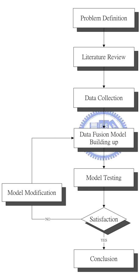
(12) 1.4 Study Flowchart. Problem Definition. Literature Review. Data Collection. Data Fusion Model Building up. Model Testing Model Modification. NO. Satisfaction. YES. Conclusion. Figure 1.4-1 Study Flowchart. 4.

(13) As shown in Figure 1.4-1, we first define the target problem. After realizing the problem, we review relevant literatures of data fusion models especially in transportation and ITS areas to understand the current developments. A data fusion model is then proposed for integrating data from different sources. A series of tests will be performed for model evaluation purpose. The testing data include both real and simulated data. According to the results of the testing experiments, model will be modified until we are satisfied. Finally, we draw some conclusions and provide some suggestions for future research.. 5.

(14) Chapter 2 Literature Review. 2.1 Review of Data Fusion Developments. 2.1.1 Introduction to Data Fusion Multi-sensor data fusion is the integration of data from multiple sensors to perform inferences which are more accurate and specific than that available by processing single-sensor data. In recent years, many data fusion approaches have been developed and applied, individually and in combination, providing users with various levels of information detail including tactical resource management, and strategic warning, as well as non-military applications. In reviewing data fusion techniques in ITS field, the techniques can be divided into three levels as follows [8]: z. First level: information processing according to single sensor or multiple sensors, this level relates to the independent data, such as instantaneous location of vehicles.. z. Second level: level two data fusion provides a higher level of inference and delivers additional interpretive meaning suggested from the raw data. At this level, correlated and integrated data are provided to the user.. z. Third level: level three data fusion is designed to make assessments and provide recommendations to the system users, much as occurs in knowledge-based expert systems (KBES). Data fusion technology started in the late 1980s and has continued to the present. It has. been given much attention in the engineering literature, yet relatively few articles discuss its potential usefulness for transportation management or ITS. In Linn and Hall’s research in 1991 [1], several common data fusion techniques are identified as Table 2.1-1 shows. And the number of available algorithms versus the primary data fusion function is as illustrated in. 6.

(15) Figure 2.1 [12]:. Table 2.1-1 Common data fusion techniques Fusion Level. General Method. Specific Technique Figure of merit (FOM). Data association Level one Positional estimation. Gating techniques Kalman filters Bayesian decision theory. Identity fusion Level two. Dempster-Schafer evidential reasoning (DSER) Adaptive neural networks. Pattern recognition. Cluster methods Expert systems. Artificial intelligence Blackboard architecture Fuzzy logic. Level three. 25. 24 20. 20 15. 15. 16. 10. 9. 5 3 0. Association Estimation number of available algorithms. Pattern Identity Fusion KnowledgeRecognition based systems. Figure 2.1 A Variety Of Algorithms Have Been Developed Which Are Readily Applicable to the ITS Data Fusion Field. 7. Other.

(16) 2.1.2 Benefits of Data Fusion According to Sarma and Raju’s 1991 research of data fusion, the benefits of multiple sensor data fusion are as follows [3]: z. Extended Spatial Coverage: One sensor can look where other sensors cannot.. z. Extended Temporal Coverage: One sensor can detect a target when other sensors cannot.. z. Increased Confidence: More than one sensor confirm to the same target.. z. Reduced Ambiguity: Joint information from multiple measurements reduces the set of hypotheses about the target.. z. Improved Detection: Integration of multiple measurements of the same target improves the assurance of the detection.. z. Robust the Performance: One sensor can contribute information when other sensors are unavailable, jammed, or broken. And the benefits are also the reference goals of data fusion researches. According to the Joint Directorate of Laboratories Data Fusion Subpanel, level two data. fusion represents an advance beyond the creation of raw sensor data, as occurs at the first level, and supports the synthesis of more meaningful information for guiding human decision-making. In this research, we will focus on level two data fusion techniques.. 2.2 Review of Level two Data Fusion Algorithms. 2.2.1 The Team Consensus Approach The team consensus approach is proposed by Albert C.S. Chung, Helen C. Shent, and Otman B. Basir in 1992 [5] [6] to integrate multisensory data. In order to enable the robots to interact with the environment more efficiently, robots are measured the physical properties such as electric, magnetic, and optical by some sensors. Since these sensors have limitations, 8.

(17) for example, bandwidth and accuracy, there exists uncertainty of the data got from them. The team consensus approach can be used to reduce the uncertainty to fuse the data. In the model, each sensor i should be given an initial utility expected function U i0 (γ ) first, where γ is the component of the possible actions set Γ ＝ (γ 1 , γ 2 ,....., γ M ) . Every U i0 (γ ) would be influenced by the others, so there needs revisal to these initial expected utility functions. That is to update the expected utility function by the following formula until every expected utility N. function converge：U ik (γ ) = ∑Wi , j (γ )U kj −1 (γ ) , Wi , j ≥ 0 , where Wi , j (γ ) is a weight assigned j =1. by sensor Si to sensor S j . In other words, the goal is to find a vector κ (γ ) = (κ 1 ,..., κ N ) so that Wi ,kj (γ ) can converge to κ (γ ) . The algorithm of finding κ (γ ) is important in this approach. This approach introduces the concept of entropy, which represents uncertainty. Entropy is a concept proposed by C. Shannon in the 1948 and is used in “ Information Theory ” first. n. The definition of entropy is： H ( p1 ,..., p n ) = −∑ p i log p i and the H ( p1 ,..., pn ) is the i =1. notation of the entropy in the sample space ( X , p1 ,..., pn ) . This approach optimizes the objective function Ri (γ ) =. ∑Wi ,2j (γ ) × h 2j|i (γ ) , subject to. s j ∈S. the optimal weighting scheme： Wi , j (γ ) =. 1 1 h (γ )∑ 2 k∈S hk |i (γ ). N. ∑W. i, j. j =1. (γ ) = 1 , Wi , j (γ ) > 0 yield. , where h 2j|i (γ ) is the. 2 j|i. conditional-entropy between sensor, Si and sensor S j . Thus, the value of the vector κ (γ ) is determined by solving the linear equation. κ (γ )W (γ ) = κ (γ ) , subject to. N. ∑ κ (γ ) = 1. i =1. i. 9.

(18) After reviewing these literatures above and [2][7], we find that entropy can be used to measure the uncertainties of sensors and the calculations of entropies are simple. We refer to the concept of entropy to form our model. 2.2.2 Introduction to Entropy. The word entropy was coined by Rudolf Clausius and was first used on thermodynamics around 1865 in Germany [9]. It was used as a measure of the amount of energy in a thermodynamics system. The word entropy was introduced to the domain of physics in 1948 when Claude Shannon was developing his theory of communication at Bell Laboratories. Let P ≡ ( p1 , p 2 ,..., p n ) T be a probability distribution associated with n possible outcomes,. denoted by X ≡ ( x1 , x 2 ,..., x n ) T . Denote its entropy by H ( p1 , p 2 ,..., p n ) . In order to reflect the uncertainty of an experiment, H ( p1 , p 2 ,..., p n ) should satisfy the axioms as follows: 1.. H ( p1 , p 2 ,..., p n ) should be a continuous function.. 2.. H ( p1 , p 2 ,..., p n ) should be a monotonically increasing function of n.. 3.. If an experiment is divided into several sub-experiments, H ( p1 , p 2 ,..., p n ) is calculated as the weighted sum of each sub-experiment.. It turns out that the unique function that satisfies these axioms has the form of n. H ( p1 , p 2 ,..., p n ) = −k ∑ p j ln p j , where k is a positive constant. Shannon chose j =1. n. − ∑ p j ln p j to represent his concept of entropy. j =1. There are some properties of entropy stated as follows: 1.. Shannon’s measure is nonnegative and concave in p1 , p 2 ,..., p n .. 2.. The inclusion of a zero-probability outcome does not change the measure.. 3.. The entropy of a probability distribution representing a completely certain outcome. 10.

(19) is 0, and that of any probability distribution representing uncertain outcomes is positive. 4.. Given any fixed number of outcomes, the maximum possible entropy is that of the uniform distribution.. 5.. The entropy of the joint distribution of two independent distributions is the sum of the individual entropies.. 6.. The entropy of the joint distribution of two dependent distributions is no greater than the sum of the two individual entropies.. 11.

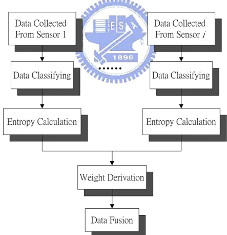
(20) Chapter 3 Model Building This section explains the principle of the proposed data fusion model. We divide the model into two parts, entropy calculation and weight derivation. The entropy measures the uncertainty and the randomness of the collected data. Classifying these data should be accomplished before calculating the entropy. The concept of data classifying is described in section 3.1. Then the concept of entropy calculating is explained in section 3.2. We use entropy to derive the weight of each sensor. Given the entropy matrix, we can determine appropriate weights for each sensor through the optimal weighting scheme. The optimal weighting scheme and the fusion result are explained in section 3.3. The flowchart of the proposed model is shown in figure 3.1.. Data Collected From Sensor 1. Data Classifying. Data Collected From Sensor i. ……. Entropy Calculation. Data Classifying. Entropy Calculation. Weight Derivation. Data Fusion. Figure 3.1 The Flowchart of the Proposed Model. 12.

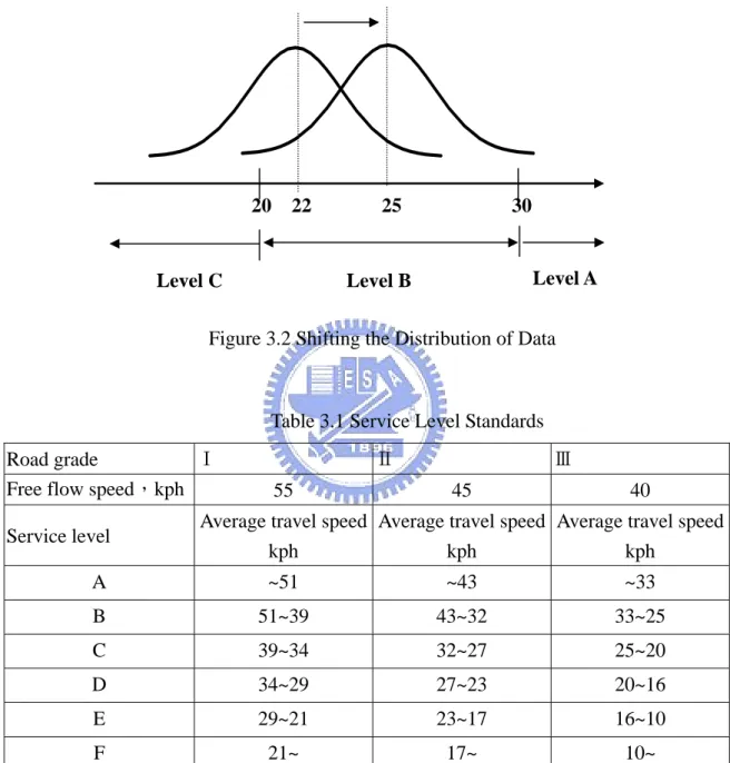
(21) 3.1 The Concept of Data Classifying We use the standards of service levels [4] to classify the collected data. The data collected from multi sensors are time mean speed, traffic volume, and position, … etc. In our model, we only consider the time mean speed. According to the range of average travel speed shown in table 3.1, we can divide the collected data into six service levels. However, six service levels are not practical to our model since the calculated entropy will be insignificant. We merge two continuous levels into one level because the difference between them is not sensitive to drivers. Also decreasing the number of service levels can reduce the complexity of the model. Adjusting the upper bounds and the lower bounds of each level slightly to make calculation easier and clearer. The new service level standards as shown in table 3.2. Sometimes the data of a sensor are classified to several service levels because its mean falls near the boundary of the service level even its standard deviation is small. In order to reduce the impacts of boundaries, we shift these data with the following steps before classifying the data: 1.. Calculate the average of the data for each sensor i, denoted by Vi;. 2.. Find the service level in the table 3.2 that Vi is belonged to;. 3.. Shift the distribution of data of each sensor i to the middle of the service level. In other words, all the data of each sensor Si are added by the difference of the mean of that service level minus Vi. If the averages of sensors fall in the different ranges of service levels, we shift all the distributions to the middle of the same range- service level B.. The classifying process can be explained in figure 3.2. According to the range of average travel speed shown in table 3.2, we categorize the shifted data into three service levels. 13.

(22) After classifying these data, we record the number of data in each level for every sensor. For example, in table 3.3, the number 24 means that there are 24 data located in service level A.. 20. 22. Level C. 25. 30. Level A. Level B. Figure 3.2 Shifting the Distribution of Data. Table 3.1 Service Level Standards Ⅰ Road grade Free flow speed，kph. Service level. Ⅱ. 55. Ⅲ. 45. 40. Average travel speed Average travel speed Average travel speed kph kph kph. A. ~51. ~43. ~33. B. 51~39. 43~32. 33~25. C. 39~34. 32~27. 25~20. D. 34~29. 27~23. 20~16. E. 29~21. 23~17. 16~10. F. 21~. 17~. 10~. 14.

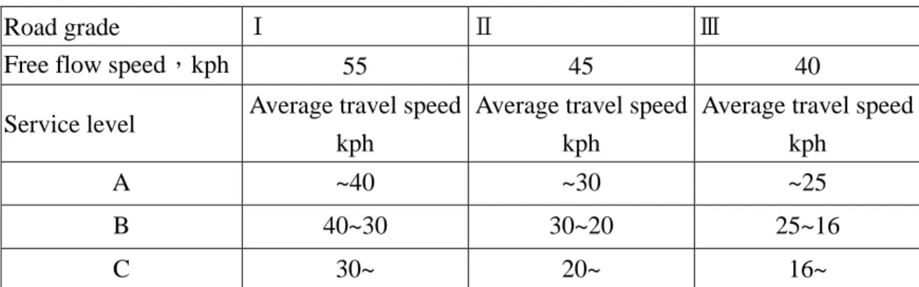
(23) Table 3.2 New Service Level Standards Ⅰ Road grade Free flow speed，kph. Service level. Ⅱ. Ⅲ. 55. 45. 40. Average travel speed Average travel speed Average travel speed kph kph kph. A. ~40. ~30. ~25. B. 40~30. 30~20. 25~16. C. 30~. 20~. 16~. Table 3.3 The Number of Data Belonged to Each Service Level for Sensor 1 Number. A. 24. B. 65. C. 48. Sum. 137. 3.2 The Concept of Entropy Calculating Entropy is a concept proposed by C. Shannon in the 1948 and is used in “ Information Theory” first. Shannon’s entropy function has been used extensively as a measure of uncertainty. We use entropy to measure the uncertainty and the randomness of the collected data. The definition of entropy is n. H ( p1 ,..., p n ) = −∑ p i log p i. (3.1). i =1. where H ( p1 ,..., pn ) is the notation of the entropy and pi is the probability of each possible outcome i. In our model, we introduce the concept of entropy with the conditional probability [5]. And we assume that any two sensors are independent. The entropy of sensor, Si, denoted by 15.

(24) hi (γ ) is given by hi (γ ) = − ∑ P(θ j | γ ) log P(θ j | γ ) θ j ∈θ. (3.2). where P (θ j | γ ) is the probability of occurrence of the state θ j given the observed state γ . In the model, γ represents the service level of the actual average speed and θ j represents the service levels of the classified data for each sensor. For example, we assume that the data in table 3.3 are collected during the time period T. If the actual service level is B, let γ equals to B. The probability of the data in service level A is 0.175 since there are 24 out of 137 data are located in service level A. Similarly, the probabilities of the data in service level B and C are 0.475 and 0.35, respectively. Notice that these probabilities are the conditional probabilities given the actual service level is B. Equation (2) can be used to calculate the entropy of sensor 1.. 3.3 The optimal weighting scheme We use entropy to derive the weight of each sensor. Given the entropy matrix, we can determine appropriate weights for each sensor through the optimal weighting scheme. For each sensor, we minimize its entropy. This implies that sensors with lower entropies will be assigned higher weights and vice versa. Since any two sensors are independent, we ignore the conditional-entropy. The conditional-entropy is a measure of the state of uncertainty of a sensor given the information of another sensor [5]. Hence, the minimization problem [5] can be adjusted as follows:. 16.

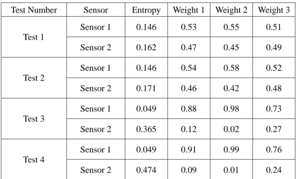
(25) Minimize. ∑ [W i∈S. 2. i. (γ )hi2 (γ )]. Subject to N. ∑ W (γ ) = 1 , i =1. i. Wi (γ ) > 0 where Wi (γ ) is the weight assigned to sensor i given the actual service level γ . Optimizing the above objective function will yield the following optimal weighting scheme:. Wi (γ ) =. 1 1 h (γ )∑ 2 j∈S h j (γ ). (3.3). 2 i. In Equation (3.3), the value of the summation term in the denominator is the same for all Wi (γ ) . Hence, the weight for each sensor is inversely proportional to the square of its entropy. The larger the entropy is, the smaller the weight assigned. However, we find that the weights are square inverse proportion to entropy and it is too exceeding. In table 3.4, weight 1 are the weights that are inverse proportion to entropy, weight 2 are the weights that are square inverse proportion to entropy, and weight 3 are the weights that are radical inverse proportion to entropy. In test 1 and test 2, the difference between the entropies of sensor 1 and sensor 2 are small, so the difference between the weights of sensor 1 and sensor 2 are also small. In test 3 and test 4, since the entropies of sensor 2 are 9~10 times larger than that of sensor 1, the differences between the weights are larger than those in test 1 and test 2. However, in the column weight 2, the difference of sensor 1 and sensor 2 is equal to 0.98-0.02=0.96, it is too exceeding. This condition is reduced in the column weight 1. The difference in the column weight 1 is equal to 0.88-0.12=0.76. Similarly, the difference is equal to 0.73-0.27=0.46 in the column weight 3. The differences are reduced from 0.96 to 0.76 and 0.46. The difference of 0.2 (0.96-0.76) is the reasonable one because the difference of 0.5 17.

(26) (0.96-0.46) is too much and may conceal the effect of entropy. So we modify it to inverse proportion to entropy. The minimization problem and equation 3.3 can be modified as follow: Minimize. ∑ [W i∈S. 2. i. (γ )hi (γ )]. Subject to N. ∑ W (γ ) = 1 , i =1. i. Wi (γ ) > 0. The optimal weighting scheme:. Wi (γ ) =. 1 1 hi (γ )∑ j∈S h j (γ ). (3.4). After calculating the weight of each sensor, we can fuse these collected data. The fusion result can be obtained by summing up the products of the average of collected data and the weight of the sensor. That is, the fusion result, denoted by V can be calculated by the following equation: N. V = ∑ WiVi. (3.5). i =1. where Vi is the average of the data for each sensor i calculated in section 3.1. Notice that Vi is the average of the data for each sensor i before we shift the data. It is different form the average of updated data.. 18.

(27) Table 3.4 The Weights of Different Weighting Schemes Test Number. Sensor. Entropy. Weight 1. Weight 2. Weight 3. Sensor 1. 0.146. 0.53. 0.55. 0.51. Sensor 2. 0.162. 0.47. 0.45. 0.49. Sensor 1. 0.146. 0.54. 0.58. 0.52. Sensor 2. 0.171. 0.46. 0.42. 0.48. Sensor 1. 0.049. 0.88. 0.98. 0.73. Sensor 2. 0.365. 0.12. 0.02. 0.27. Sensor 1. 0.049. 0.91. 0.99. 0.76. Sensor 2. 0.474. 0.09. 0.01. 0.24. Test 1. Test 2. Test 3. Test 4. 19.

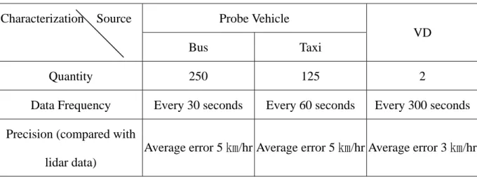
(28) Chapter 4 Model Testing In this section, we perform a series of tests for model evaluation purpose. The sources of urban traffic information are loops, probe vehicles, VD, …,etc. and we only consider probe vehicles and VD in the testing. We collect lidar data and data from other sources simultaneously. The lidar data is considered as the correct data and is compared with the fusing result of our model. However, collecting real data is hard in practice and the volume of real data is often small. Thus, we also use simulated data to test our model. The data collection, generation, and analysis are explained in section 4.1. We use these data as the input of our data fusion model. The steps of calculating the entropies and deriving the weights are explained in section 4.2.Finally, we explain the fusion results and compare them with the lidar data in section 4.2.. 4.1 Data Collection and Generation Probe vehicles and VD are the sources of urban traffic information used in our testing. The characterizations of these sources are as follows:. Table 4.1 Properties of probe vehicles and VD. Characterization Source. Probe Vehicle VD Bus. Taxi. Quantity. 250. 125. 2. Data Frequency. Every 30 seconds. Every 60 seconds. Every 300 seconds. Precision (compared with Average error 5 ㎞/hr Average error 5 ㎞/hr Average error 3 ㎞/hr lidar data). 20.

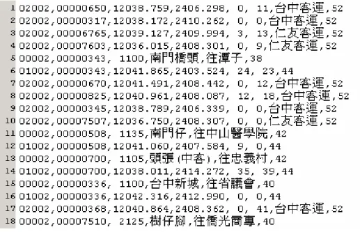
(29) 4.1.1 Dynamic Bus Information Acquirement and Analysis. The dynamic bus information is provided by Taichung City Government. The information includes ID of on board units, name of the public transit company, route ID, name of the terminal stations, and speeds. The data updates every 30 seconds. The data processing can be divided into two parts, data reading and data filtration. The steps of the data processing are explained as follows: 1. Data reading: The information of the Taichung city bus is given in string format as shown in figure 4.1. Each item is separated by a comma. The first item is “ ID of the on board unit”, “ name of the public transit company and the route of the bus”, “ name of the next approaching station”, “ name of the terminal station”, “longitude”, “latitude”, and “ azimuth of the bus”. 2. Data filtration: The speeds decrease while buses stop to pick up and drop passengers. Hence, some of these speeds are too low to reflect the real travel speed. There are many relevant paper discuss methods to filter low speed data. Almost every method requires large amount of data. However, the data we collected are too low in volume to use these methods. So we simply delete the speed which is lower than 5 ㎞/hr.. 21.

(30) Figure 4.1 The Raw Data of Taichung City Bus Dynamic Information.. 4.1.2 Dynamic Taxi Information Acquirement and Analysis. The dynamic taxi information is provided by Geda Telecommunication Co., Ltd. The information includes time, longitude and latitude coordinates, speeds, ID of on board units, and azimuth. The data updates every 60 seconds. The data processing of dynamic taxi information is similar to that of dynamic bus information. The data reading and data filtration process are explained as follows: 1. Data reading: The raw data of the taxi information is given in string format as shown in figure 4.2. Each item is separated by comma. The first item is “time”, the second item is “longitude”, and the following items are “latitude”, ”speed”, ”ID of the on board unit”, ”azimuth”, and “ID of a specific road”. 2. Data filtration: Taxi also has to stop to pick up and drop passengers and these stops cause low-speed. 22.

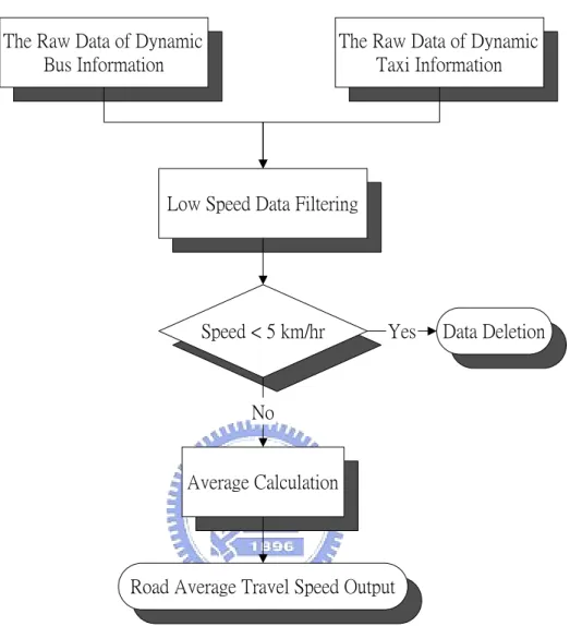
(31) data. As the same reason of processing bus data, the amount of data is not large enough to use filter methods found in literatures. So we still use the simple rule by deleting data whose speed is lower than 5 ㎞/hr.. We regard the bus data and the taxi data as the same probe source. So we merge the filtered bus data and taxi data into one. We calculate the average of the merged data and it is the representation speed of the road provided by probe vehicles. The process of probe vehicle speed filtering is as shown in figure 4.3.. Figure 4.2 The Raw Data of Dynamic Taxi Information (Provided by Geda Telecommunication Co., Ltd.). 23.

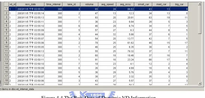
(32) The Raw Data of Dynamic Bus Information. The Raw Data of Dynamic Taxi Information. Low Speed Data Filtering. Speed < 5 km/hr. Yes. Data Deletion. No. Average Calculation. Road Average Travel Speed Output. Figure 4.3 The Probe Vehicle Speed Filtering.. 4.1.3 Dynamic VD Information Acquirement and Analysis. We use VD as the source of detectors. The raw data of VD is shown in figure 4.4. The first column is the ID of the VD, and the following columns are time of the latest received data, data sending cycle, ID of the lane, traffic volume, average travel speed, average occupancy, volume of small cars, volume of middle cars, and volume of large cars. The VD is installed near an intersection. When the vehicle is stopped by the traffic light, the data obtained from VD is not usable. So we delete the data whose speed are lower than 5 ㎞/hr. 24.

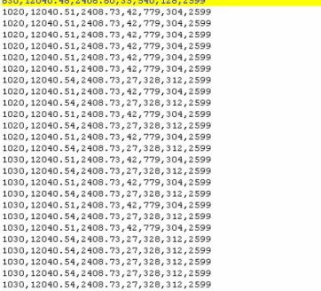
(33) Based on our experiences, we sometimes find extraordinary and isolated data which is much higher than the average speed. We suspect these abnormal data is due to the mechanical failure or some other reason. So we also delete the speeds which are higher than 80 km/hr. We calculate the average of the remaining VD data and it is the representation speed of the road provided by detectors. The process of VD data filtering is as shown in figure 4.5.. Figure 4.4 The Raw Data of Dynamic VD Information.. 25.

(34) The Raw Data of Dynamic VD Information. Data Filtering. Speed < 5 km/hr or Speed > 80 km/hr. Yes. Data Deletion. No Average Calculation. Road Average Travel Speed Output. Figure 4.5 The VD Speed Filtration.. 4.1.4 Data Simulation and Analysis. Since collecting real data is hard in practice and the volume of real data is often small, we also use simulated data to test our model. The simulated data is expected to follow the same distribution as that of the data we collected from real sensors. So we perform the goodness-of-fit test to find the distribution of real data. We find that the real data is following normal distribution. We assume the length of the target road is 360 meters and the buses’ arrival follow Poison distribution. The arrival rate of buses is 0.5 per minute and the frequency of data 26.

(35) sending is 4 times per minute. The speed follows normal distribution and the average speed and standard deviation are adjustable. The simulation time lasts for 2 hours. We use the similar way to simulate data obtained from VD. The additional assumption is that the arrival rate of vehicle is 10 per minute. We adjust the average and standard deviation to generate data representing different service levels. The different service level scenario can represent different situations in the real world in order to have more comprehensive test. The simulation process of the probe vehicle data is explained in figure 4.6. In this flowchart, tj is the time when the probe vehicle sending its GPS data to the center. Total distance is the length of the target road and its initial value is 360 meters. T is the simulation time, which is set to be 10800 seconds. Vj is the average speed during the time period tj - tj-1. The simulation process of the VD data is explained in figure 4.7. In the flowchart, ti and Vj are the time and speed, respectively when a vehicle passes by VD; T is the simulation time and it is set to be10800 seconds.. 27.

(36) Generate time t 0 of a bus with the arrival rate 0.5 per minute which follows Poison distribution. Total distance=Total distance - (t 0 x average speed) ; j=1. tj=tj-1 +15. tj > T. Yes. Stop simulating. No. Total distance >0. No. Stop simulating this bus. Yes. Generate speed V j. Total distance=Total distance - (15 x Vj ) ; j++. Figure 4.6 The Flowchart of Simulate Probe Vehicle Date.. 28.

(37) Generate time t i of a vehicle with the arrival rate 10 per minute which follows Poison distribution. t = t + ti. t>T. Yes. Stop simulating. No Generate speed V i. Figure 4.7 The Flowchart of Simulate VD Date.. 4.2 Model Testing Implementations In this section, we use both real data and simulated data to test our model. Section 4.2.1 explains the fusing steps using real data and section 4.2.2 explains those using simulated data. 4.2.1 Model Testing Using Real Data. Some descriptions of real data are as follows: 1.. Collection time: November 14, 2003. P.M. 16:00 ~ P.M.19:00.. 2.. Collection site: Taichung Chung Cheng Road (near the intersection of Taichung Harbor Road).. 3.. Collected Data: The real data collected include probe vehicle data and VD data. The probe vehicle data are composed of bus speeds and taxi speeds.. The steps of calculating the entropies and deriving the weights are explained as follows: Step 1:. 29.

(38) We use the definitions of service levels in table 3.2 to classify the collected data. The result of classification is shown in table 4.2.1 and table 4.2.2. The average speeds of probe vehicle data and VD data are 21.88 km/hr and 23.91 km /hr, respectively.. Table 4.2.1 The Amount of the Prove Vehicle Data Service Level. Amount. A. 24. B. 65. C. 48. Total. 137. Table 4.2.2 The Amount of the VD Data Service Level. Amount. A. 7. B. 19. C. 7. Total. 33. Step 2: There are 1636 lidar data and the average of these data is 27.39 km /hr. That means the (real) service level of our test site is B. Hence, the γ in equation 3.2 can be represented by Bˆ . Then we calculate the probability of occurrence of the state θ j given the observed state Bˆ for each sensor. The probability is given by. P(θ j | Bˆ ) ,. θ j =A,B,C,…. 30.

(39) Let’s take probe vehicle data as an example to illustrate how to calculate these probabilities. P ( A | Bˆ ) represents the probability that the service level of the probe vehicle data is A when the actual service level is B, which is equals to. 24 = 0.175. The 24 + 65 + 48. other calculation results of probabilities are shown in table 4.2.3 and table 4.2.4.. Table 4.2.3 The Conditional Probabilities of the Prove Vehicle Data Service Level. Probability. P ( A | Bˆ ). 0.175. P ( B | Bˆ ). 0.475. P (C | Bˆ ). 0.350. Total. 1. Table 4.2.4 The Conditional Probabilities of the VD Data Service Level. Probability. P ( A | Bˆ ). 0.212. P ( B | Bˆ ). 0.576. P (C | Bˆ ). 0.212. Total. 1. Then we use equation 3.2 to calculate the entropy of each sensor. h1 ( B) represents the entropy of probe vehicle when the real service level is B, which is equals to −. ∑ P (θ. θ j ∈θ. j. | B ) log P (θ j | B ) = −(0.175 log 0.175 + 0.475 log 0.475 + 0.35 log 0.35) = 0.446 .. The results of entropy calculating are shown in table 4.2.5. 31.

(40) Table 4.2.5 The Entropy of Each Sensor Sensor. Entropy. Probe Vehicle. 0.446. VD. 0.424. Step 3: Given the entropies, we can determine appropriate weights for each sensor through equation 3.4. W1 ( B) represents the weight of probe vehicle when the real service level is B, which is equals to. 1 ⎛ 1 1 ⎞ ⎟⎟ h1 ( B)⎜⎜ + ⎝ h1 ( B) h2 ( B) ⎠. =. 1 1 ⎞ ⎛ 1 + 0.446⎜ ⎟ ⎝ 0.446 0.424 ⎠. = 0.487 . The calculation. results are shown in table 4.2.6.. Table 4.2.6 The Optimal Weight of Each Sensor Sensor. Weight. Probe Vehicle. 0.487. VD. 0.513. Step 4: After calculating the weight of each sensor, we can fuse these collected data. The fusion result can be obtained by summing up the products of the average of collected data and the weight of the associated sensor. So the fusing result is:. 21.88 × 0.487 + 23.91× 0.513 = 22.92. km /hr. The difference between the fusing result and the real speed collected from lidar is equals to 27.39－22.92＝4.47 km/hr. Since the standard deviation of the lidar data is 7.125 km/hr and the difference 4.47 km/hr which falls within the range of the standard deviation. Generally speaking, we consider it is an acceptable difference. 32.

(41) 4.2.2 Model Testing Using Simulated Data. We use different scenarios to represent different service levels in the real world. These scenarios have different averages or standard deviations. Since the calculation procedures are the same, we only show the results of each step in this section. There are seven testing scenarios as follows: 1.. Two sensors with same average and standard deviation.. 2.. Two sensors with same standard deviation and small difference of averages. We use the same simulated data of sensor 1 and replace the data of sensor 2 by the data with different average.. 3.. Two sensors with same standard deviation and large difference of averages. Similar to test 2, we replace the data of sensor 2 by the data with different averages.. 4.. Two sensors with same average and small difference of standard deviations. We simulate two new sets of data which have same average with different standard deviations.. 5.. Two sensors with same average and large difference of standard deviations. Similar to test 4, we replace the data of sensor 2 by the data with large difference of standard deviation.. 6.. Two sensors with different averages and standard deviations. We test our model with two data sets which have different averages and standard deviations. 7.. Three sensors with same average and different standard deviations. We use three data sets to test our model. These data have same average with different standard deviations.. 33.

(42) The average speeds and standard deviations of sensor 1(simulate probe vehicle data), sensor 2(simulate VD data), and sensor 3(simulate VD data) for each test are shown in table 4.2.7.. Table 4.2.7 Averages and Standard Deviations of Sensors Test Number. Sensor. Average Speed. Standard Deviation. Sensor 1. 25.07. 2.91. Sensor 2. 25.06. 2.96. Sensor 1. 25.07. 2.91. Sensor 2. 21.97. 3.02. Sensor 1. 25.07. 2.91. Sensor 2. 14.95. 2.98. Sensor 1. 25.15. 1.98. Sensor 2. 24.92. 5.02. Sensor 1. 25.15. 1.98. Sensor 2. 24.72. 10.04. Sensor 1. 25.07. 2.91. Sensor 2. 22.05. 5.05. Sensor 1. 24.91. 1.05. Sensor 2. 25.07. 2.96. Sensor 3. 24.92. 5.02. Test 1. Test 2. Test 3. Test 4. Test 5. Test 6. Test 7. 34.

(43) The results of shifting the averages to the middle of the service level and classifying are shown in table 4.2.8.. Table 4.2.8 The Amount of Data Test Number. Sensor. Service Level A. Service Level B. Service Level C. Total. Sensor 1. 9. 239. 12. 260. Sensor 2. 123. 2173. 100. 2396. Sensor 1. 9. 239. 12. 260. Sensor 2. 113. 2152. 126. 2391. Sensor 1. 9. 239. 12. 260. Sensor 2. 102. 2126. 109. 2373. Sensor 1. 2. 144. 1. 147. Sensor 2. 381. 1640. 374. 2395. Sensor 1. 2. 144. 1. 147. Sensor 2. 720. 906. 696. 2322. Sensor 1. 9. 239. 12. 260. Sensor 2. 396. 1636. 395. 2427. Sensor 1. 267. 0. 0. 267. Sensor 2. 123. 2173. 100. 2396. Sensor 3. 381. 1640. 374. 2395. Test 1. Test 2. Test 3. Test 4. Test 5. Test 6. Test 7. 35.

(44) We assume the real travel speed is in service level B. The conditional probabilities can be calculated as shown in table 4.2.9.. Table 4.2.9 The Conditional Probabilities of Each Sensor. Test Number. Sensor. P ( A | Bˆ ). P ( B | Bˆ ). P (C | Bˆ ). Total. Sensor 1. 0.0346. 0.9192. 0.0462. 1. Sensor 2. 0.0513. 0.9070. 0.0417. 1. Sensor 1. 0.0346. 0.9192. 0.0462. 1. Sensor 2. 0.047. 0.9. 0.053. 1. Sensor 1. 0.0346. 0.9192. 0.0462. 1. Sensor 2. 0.043. 0.911. 0.046. 1. Sensor 1. 0.0136. 0.9796. 0.0068. 1. Sensor 2. 0.159. 0.685. 0.156. 1. Sensor 1. 0.0136. 0.9796. 0.0068. 1. Sensor 2. 0.310. 0.390. 0.30. 1. Sensor 1. 0.0346. 0.9192. 0.0462. 1. Sensor 2. 0.163. 0.674. 0.163. 1. Sensor 1. 1. 0. 0. 1. Sensor 2. 0.0513. 0.9070. 0.0417. 1. Sensor 3. 0.159. 0.685. 0.156. 1. Test 1. Test 2. Test 3. Test 4. Test 5. Test 6. Test 7. 36.

(45) Then we use equation 3.2 to calculate the entropy of each sensor and the results are shown in table 4.2.10.. Table 4.2.10 The Entropy of Each Sensor Test Number. Sensor. Entropy. Sensor 1. 0.146. Sensor 2. 0.162. Sensor 1. 0.146. Sensor 2. 0.171. Sensor 1. 0.146. Sensor 2. 0.157. Sensor 1. 0.049. Sensor 2. 0.365. Sensor 1. 0.049. Sensor 2. 0.474. Sensor 1. 0.146. Sensor 2. 0.372. Sensor 1. 0.0001. Sensor 2. 0.1622. Sensor 3. 0.365. Test 1. Test 2. Test 3. Test 4. Test 5. Test 6. Test 7. 37.

(46) We can determine weights for each sensor through equation 3.4. The calculation results are shown in table 4.2.11.. Table 4.2.11 The Optimal Weight of Each Sensor Test Number. Sensor. Weight. Sensor 1. 0.527. Test 1. 1 Sensor 2. 0.473. Sensor 1. 0.54. Sensor 2. 0.46. Sensor 1. 0.519. Sensor 2. 0.481. Sensor 1. 0.882. Test 2. 1. Test 3. 1. Test 4. 1 Sensor 2. 0.118. Sensor 1. 0.907. Test 5. 1 Sensor 2. 0.093. Sensor 1. 0.719. Sensor 2. 0.281. Sensor 1. 0.9991. Sensor 2. 0.0006. Sensor 3. 0.0003. Test 6. Test 7. Total. 1. 38. 1.

(47) The fusing results of each test are shown in table 4.2.12:. Table 4.2.12 Fusing Results of Each Test Test Number. Fusing Result. Test 1. 25.07 × 0.527 + 25.06 × 0.473 = 25.07. Test 2. 25.07 × 0.54 + 21.97 × 0.46 = 23.64. Test 3. 25.07 × 0.519 + 14.95 × 0.481 = 20.20. km /hr. Test 4. 25.15 × 0.882 + 24.92 × 0.118 = 25.12. km /hr. Test 5. 25.15 × 0.907 + 24.72 × 0.093 = 25.11. km /hr. Test 6. 25.07 × 0.719 + 22.05 × 0.281 = 24.22. km /hr. Test 7. 24.91× 0.9991 + 25.07 × 0.0006 + 24.92 × 0.0003 = 24.91. km /hr km /hr. km /hr. We can find that entropy can reflect the uncertainty of a sensor. That is, when the standard deviation is large, the entropy tends be large. Then we will assign lower weight to the sensor.. 4.3 Conclusions About Fusion Results According to the results of the tests in section 4.2 and 4.2, we draw some conclusions as follows: 1. The probe vehicle data is small in volume and sometimes the historical database is needed. 2. The entropy of VD data is smaller than that of the probe vehicle data, so the VD is considered a more reliable source than probe vehicles. 3. The average speeds of lidar data are sometimes high since we do not detect motionless. 39.

(48) vehicles. So the fusion result is lower than the average of lidar data. 4. The entropy is sensitive to the dispersion of data. That is, when the standard deviation of data of a sensor is slightly larger than that of another sensor, the entropy of the former is much larger than that of the latter. 5. The high entropies are sometimes due to the classification standards. Even the standard deviations of the two sensors are same, the entropies of them may be significant different. These cases can be reduced through shifting the distribution of data of each sensor to the middle of the service level. 6. When the averages of sensors are significant different, we can’t know which of the sensor is accurate. So the sensors should be checked their accuracy before fusion.. 40.

(49) Chapter 5 Conclusions and Suggestions In this section, we offer some conclusions and some suggestions regarding this research. Section 5.1 and 5.2 discuss conclusions and suggestions, respectively.. 5.1 The Conclusions We draw some conclusions about our model as follows: 1.. According to the testing results, our model is suitable in general. Entropies represent the uncertainties of sensors. There is no requirement that these sensors must have the same amount of data.. 2.. Our model can be used to reflect sudden changes of speeds. The changes of traffic conditions are considered continuance. However, a sudden change in speed during a short period of time sometimes occurs. We use scenarios of different standard deviations to simulate the changes of speeds. We find that the entropy is high when standard deviation is large and vice versa. Hence, the sudden changes of speeds can be reflected by entropy.. 3.. This approach is used to reflect the irregular degree of data and can’t represent the accuracy of data. That is, when the whole data of a sensor are lower or higher than the normal speed, entropy cannot reveal this fact.. 4.. Sometimes the value of entropy is influenced by the classification standards. In our model, these cases can be reduced through shifting the distribution of data of each sensor to the middle of the service level.. 5.. This approach can be extended to multi-source data fusion. The entropy is calculated through the probabilities of classified data of the target sensor and has no relationship with the probabilities of other sensors. Hence, there is no limitation in the number of sensors in this fusion model.. 41.

(50) 6.. The fusion result is close to the average of the data of sensors when the averages of each sensor are in small difference.. 7.. The effect of entropy is obvious when the variations of data are large. The entropy is large when the variation of data is large and vice versa. When the entropy of a sensor is much larger than others, its weight is obviously smaller than others.. 5.2 The Suggestions In this section, we offer some suggestions about data fusion for the future researches stated as follows: 1.. To address weakness of entropy failing to reflect whether the row data is correct or not, we can consider another variable while calculating the weights. For example, use the historical database to acquire the average speed during a specific time period. We can compare the average of historical data and the average of the fused data. If the difference between these two averages is large, we can adjust the entropy value. Then the weights can reflect the accuracy of sensors.. 2.. We use the average of lidar data as the accurate value to compare with our fusing results. However, the lidar data is another source of traffic information and there are also errors when we acquire them. If the research time and funds are enough, the video camera may be a more accurate source for comparison purpose.. 3.. The classifying method can be modified. Shifting the distribution of data of each sensor to the middle of the service level can solve a portion of the problem due to the classification standards. However, there still room for modifying the classification standards to reduce its impacts.. 4.. The filtering method is too simple. Since the emphasis on our model is the fusion method, we do not spend sufficient time on surveying the filtering method of the raw data. So we simply filter out the exceeding values. The fusion model will be a 42.

(51) more complete one if there is a better filtering algorithm. 5.. The optimal weight scheme can be modified. According to some results of experiments, we conclude that the weight of a sensor is inverse proportion to its entropy. However, there may be other factors that we do not discover which influence the relationship between entropy and weight. Future researches can modify the optimal weight scheme to reflect these factors.. 43.

(52) Reference [1] Linn, R.J. and D.L. Hall. “A Survey of Multi-sensor Data Fusion Systems.” Proceedings ofthe SPIE - The International Society for Optical Engineering. 1-2 April 1991: Orlando, FL.SPIE, 1991. Vol. 1470: (13-29). [2] B. Fassinut-Mombot, J.B. Choquel, ” An Entropy Method For Multisource Data Fusion”, ISIF,2000. [3] Sarma, V.S. and S. Raju. “Multisensor Data Fusion and Decision Support for Airborne Target Identification.” IEEE Transactions on Systems, Man and Cybernetics. Sept.-Oct. 1991: (1224-30). [4] Ministry of Transportation and Communications in Taiwan, Highway Capacity Manual, 1991. [5] Albert C.S. Chung, Helen C. Shen, Otman B. Basir, ”A Decentralized Approach to Sensory Data Integration” ,IEEE,1997. [6] Otman B. Basir, Helen C. Shen, “Sensory Data Integration: A Team Consensus Approach”, IEEE, 1992. [7] Yifeng Zhou, Henry Leung, ”Minimum Entropy Approach for Multisensor Data Fusion”, IEEE,1997. [8] Daniel J. Dailey, Patricia Harn, and Po-Jung Lin, “The Final Research Report of ITS Data Fusion”, Washington State Transportation Center and Washington State Department of Transportation, April 1996. [9] Shu-Cherng Fang, J.R. Rajasekera, H.S.J. Tsao, “Entropy Optimization and Mathematical Programming”, International Series in Operations Research & Management Science, 1997. [10] Ruey Long Cheu, Der-Horng Lee, and Chi Xie, “An Arterial Speed Estimation Model Fusing Data from Stationary and Mobile Sensors”, IEEE,2001. [11] John N. Ivan, ”Data Fusion of Fixed Detector and Probe Vehicle Data for Incident Detection”, Computer-Aided Civil and Infrastructure Engineering,1998. 44.

(53) [12] David Keever, James Pol, ”Data Fusion To Support Information Needs for Surface Transportation Operations”, The 9th World Congress on Intelligent Transport Systems, 2002. [13] Zhaosheng Yang, Feng Jian, Lixia Bao, ”Study on the data fusion technology in advanced public transportation system”, China’s 10th Five-Year National Key Technologies R&D Program, 2002. [14] Daniel J. Dailey, “Sensor Data Fusion within a Regional Architecture for ITS Applications”, Proceedings of the Intelligent Vehicles '95 Symposium, 1995. [15] Simon Nash, Ray Morris, Tom Cherrett, “Management of Journey Time Data in an Integrated Traffic Control System”, The 6th ITS World Congress, 1999. [16] Bruce Hellinga, Rajesh Gudapati, “Estimating Link Travel Times from Different Data Sources for Use in ATMS and ATIS ”, Proceedings of the Canadian Society of Civil Engineers 3rd Transportation Specialty Conference held in London, Ontario, 2000. [17] Shawn M. Turner, Douglas J. Holdener, “Probe Vehicle Sample Sizes for Real-Time Information: The Houston Experience”, IEEE, 1995. [18] Bruce R. Hellinga, Liping Fu, “Reducing bias in probe-based arterial link travel time estimates”, Transportation Research Part C, 2002. [19] Ashish Sen, Piyushimita (Vonu) Thakuriah, Xia-Quon Zhu, Alan Karr, “Variances of Link Travel Time Estimates: Implications for Optimal Routes”, Internal Transportations in Operational Research, 1999. [20] Hui-Wen Chang, “The Study of Using GPS Data of Buses to Estimate the Average Speed in a Link”, Thesis of Master of NCTU, 2002.. 45.

(54)