一個使用多層串流技術之轉碼器架構設計於精細可調層次式到MPEG-1/2/4單一層次式的位元流轉碼應用

全文

(1)國立交通大學電子工程學系電子研究所碩士班碩士論文. 一個使用多層串流技術之轉碼器架構設計於精細可調層次式到MPEG-1/2/4單一層次式的位元流轉碼應用 A FGS-to-MPEG-1/2/4 Single-Layer Transcoder with Multi-Layer Streaming Techniques. 研究生：陳韋霖指導教授：蔣迪豪博士. 中華民國九十五年七月 i.

(2) 一個使用多層串流技術之轉碼器架構設計於精細可調層次式到MPEG-1/2/4單一層次式的位元流轉碼應用 A FGS-to-MPEG-1/2/4 Single-Layer Transcoder with Multi-Layer Streaming Techniques 研究生：陳韋霖. Student: Wei-Lin Chen. 指導教授：蔣迪豪博士. Advisor: Dr. Tihao Chiang. 國立交通大學電子工程學系電子研究所碩士班碩士論文. A Thesis Submitted to Department of Electrical Engineering & Institute of Electronics College of Electrical Engineering and Computer Science National Chiao-Tung University in Partial Fulfillment of the Requirements for the Degree of Master in Electronics Engineering June 2006 Hsinchu, Taiwan, Republic of China. 中華民國九十五年七月 ii.

(3) 一個使用多層串流技術之轉碼器架構設計於精細可調層次式到MPEG-1/2/4單一層次式的位元流轉碼應用研究生：陳韋霖. 指導教授：蔣迪豪博士. 國立交通大學電子工程學系電子研究所碩士班. 摘. 要. 本篇論文提出一個精細可調層次式到MPEG-1/2/4單一層次式的位元流轉碼器架構，並應用兩個新發展的轉碼技術以改善現有異質環境轉碼的。多層轉碼技術藉由傳送額外的加強層來補償異質性轉碼中的所造成的嚴重錯誤傳遞問題。位元率-失真最佳化模型則在有限的通道頻寬下，提供一個在編碼效能以及傳輸位元率之間最佳平衡點的編碼決策。實驗結果顯示所提出的使用多層轉碼技術的轉碼架構與一般的架構相比較能夠提供非常良好的轉碼效能。整合所提出的冪次位元率-失真模型以及多層轉碼技術，我們所提出的轉碼器架構，與被視為擁有最低轉碼複雜度之一的簡化餘弦轉換域轉碼架構相比較，可達到最多5.8dB的影像訊號雜訊比改善，且幾乎不增加其轉碼複雜度。與另一種擁有最佳轉碼品質的串接餘弦轉換域轉碼架構相比，我們所提出的多層轉碼技術的轉碼架構在低位元率時有相近的視訊品質，在高位元率時有0.2–1.4dB的影像訊號雜訊比損失，但轉碼複雜度上只需其34.17%的計算複雜度。. iii.

(4) A FGS-to-MPEG-1/2/4 Single-Layer Transcoder with Multi-Layer Streaming Techniques Student: Wei-Lin Chen. Advisor: Dr. Tihao Chiang. Department of Electronic Engineering & Institute of Electronics National Chiao-Tung University. Abstract In this thesis, we proposed a Fine Granularity Scalable (FGS) multi-layer to MPEG-1/2/4 single-layer transcoding framework and used two new techniques, multi-layers transcoding and R-D optimization modeling, to improve the poor performance in heterogeneous transcoding. The multi-layer transcoding technique provided heterogeneous drift error compensation via transmitting an additional enhancement layer. The rate-distortion optimization modeling is used to achieve a better tradeoff point between coding efficiency and transmission bit rate under limited channel bandwidth. The experimental results showed the proposed Multi-layer Simplified DCT-Domain Transcoder (MSDDT) architecture can provide a very good transcoding performance compared to the conventional architectures. With the proposed power-law R-D modeling in the proposed multi-layer transcoding techniques, the proposed framework shows up to 5.8 dB PSNR gains over the SDDT architecture under the similar transcoding complexity. Compared to the Cascaded DCT-Domain Transcoder (CDDT) architecture, the MSDDT architecture has similar PSNR quality at low bit rate and about 0.2–1.4 dB loss in PSNR at high bit rate, but with only keeping 34.17% complexity compared with cascaded decoder-encoder (DEC-ENC) architecture.. iv.

(5) 誌謝研究所的兩年間，論文的完成，實在是仰賴很多人的協助與指導，在此獻上誠摯的感謝。首先要感謝我的指導教授蔣迪豪老師，在研究的領域給了我很多建議與幫助。感謝實驗室的俊能學長，文孝學長，士豪學長，項群學長和志鴻學長，對於我的論文研究提出寶貴的意見與建議。雖然我的研究主題歷經很長一段混沌未明的階段，士豪學長還是在百忙之中抽空，指導了我很多，關於研究的方向以及研究的態度。雖然我常常達不到學長要求的標準，他還是不厭其煩的給我意見與指導，在這裡我要說聲感謝。另外，感謝實驗室的所有同學，讓我度過了很愉快的兩年研究所生活。感謝支持我的家人，雖然我很少抽的出時間回家，但家人的鼓勵與關懷是支撐我最大的動力。感謝所有幫助過我的朋友，因為有你們，讓我在艱難與考驗中成長。最後，僅以這篇論文，獻給所有陪我走過這一段日子的人，謝謝。. v.

(6) Contents 中文摘要 ......................................................................................................................... iii Abstract.............................................................................................................................iv 誌謝 ................................................................................................................................v Contents............................................................................................................................vi List of Tables................................................................................................................. viii List of Figures...................................................................................................................ix List of Notations ............................................................................................................. xii Chapter 1 Introduction.......................................................................................................1 1.1. Overview of MPEG-21 Transcoding Systems .................................................... 1 1.2. Scope of This Thesis ........................................................................................... 2 Chapter 2 State of the Art..................................................................................................4 2.1. Transcoding Architectures................................................................................... 4 2.1.1. Spatial-Domain Video Transcoding ............................................................4 2.1.2. Frequency-Domain Video Transcoding ......................................................7 2.2. Video Transcoding Techniques......................................................................... 13 2.2.1. Intra-Refresh Technique............................................................................13 2.2.2. Rate Control Issues....................................................................................15 2.3. Evaluation of Transcoding Architectures.......................................................... 15 2.3.1. Complexity Analysis .................................................................................16 2.3.2. Drift Error Analysis...................................................................................16 2.3.3. Evaluation and Discussion ........................................................................19 Chapter 3 FGS to Single-Layer Transcoder ....................................................................21 3.1. Multi-Layer to Single-Layer Transcoding Framework ..................................... 21 3.2. Design Issues of Heterogeneous Transcoding................................................... 25 vi.

(7) Chapter 4 Multi-Layer Transcoding Approach ...............................................................29 4.1. Drift Compensation with Additional Enhancement Layer................................ 29 4.2. Multi-Layer Transcoding with R-D Optimization ............................................ 32 Chapter 5 Experimental Results ......................................................................................41 5.1. Test Conditions.................................................................................................. 41 5.2. Rate-Distortion Performance............................................................................. 42 5.2.1. MPEG-4 FGS to MPEG-1.........................................................................42 5.2.2. MPEG-4 FGS to MPEG-2.........................................................................47 5.2.3. MPEG-4 FGS to MPEG-4 SP ...................................................................56 5.3. Complexity Analysis ......................................................................................... 65 5.3.1. Module-wise Comparison .........................................................................65 5.3.2. Arithmetic Operations Comparison...........................................................66 Chapter 6 Conclusion ......................................................................................................71 Reference .........................................................................................................................73. vii.

(8) List of Tables Table 1. Matrices Hi and Gi .................................................................................................8 Table 2. Complexity analysis of four transcoding architectures .......................................16 Table 3. Different types of drift error................................................................................18 Table 4. Drift error analysis of four transcoding architectures .........................................19 Table 5. A summary of the toolsets in MPEG-1, MPEG-2, and MPEG-4........................26 Table 6. RMSE of the estimation of the (R, αopt) relationship using different models .....35 Table 7. Rate-distortion comparison for FGS-to-MPEG-1 transcoding ...........................47 Table 8. Rate-distortion comparison for FGS-to-MPEG-2@MP transcoding ..................48 Table 9. Rate-distortion comparison for FGS-to-MPEG-4@SP transcoding ...................64 Table 10. Module-wise complexity comparison of six transcoding architectures ............65 Table 11. Instructions required per block for each module...............................................66 Table 12. Arithmetic complexity ratio for the six transcoding architectures compared to the DEC-ENC architecture. ...................................................................................68. viii.

(9) List of Figures Fig. 1. Video transcoding operations...................................................................................2 Fig. 2. Cascaded decoder and encoder transcoder...............................................................2 Fig. 3. Cascaded Pixel-Domain Transcoder (CPDT) ..........................................................5 Fig. 4. Motion vector composition ......................................................................................6 Fig. 5. Source block extraction problem .............................................................................7 Fig. 6. Cascaded DCT-Domain Transcoder (CDDT)........................................................10 Fig. 7. Simplified DCT-Domain Transcoder (SDDT).......................................................13 Fig. 8. Open-loop transcoder .............................................................................................13 Fig. 9. Intra refresh in open-loop architecture...................................................................14 Fig. 10. FGS to single-layer CDDT...................................................................................22 Fig. 11. FGS to single-layer transcoder.............................................................................24 Fig. 12. Corresponding FGS encoder framework for MSDDT.........................................30 Fig. 13. Multi-layer Simplified DCT-Domain Transcoder (MSDDT)..............................32 Fig. 14. General curve behaviors for different models......................................................35 Fig. 15. MSE vs. bit rate when running MSDDT with various α, and R combinations for Akiyo (upper left), Foreman (upper right), Mobile (lower left), and Stefan (lower right) at 256-Kbps BL bit rate ...............................................................................36 Fig. 16. MSE vs. bit rate when running MSDDT with various α, and R combinations for Akiyo (upper left), Foreman (upper right), Mobile (lower left), and Stefan (lower right) at 512-Kbps BL bit rate ...............................................................................36 Fig. 17. MSE vs. bit rate when running MSDDT with various α, and R combinations for Akiyo (upper left), Foreman (upper right), Mobile (lower left), and Stefan (lower right) at 1024-Kbps BL bit rate .............................................................................37. ix.

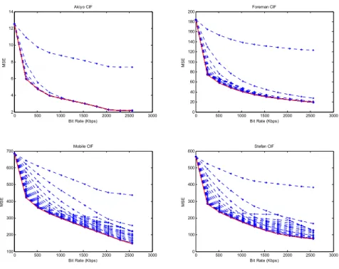
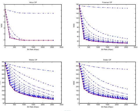
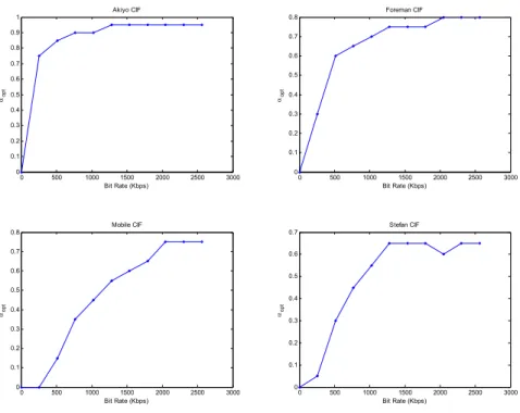
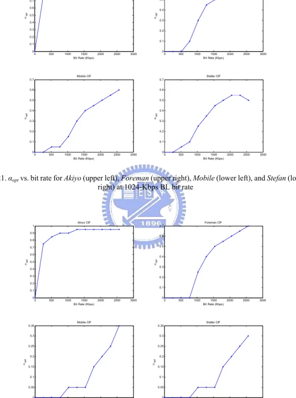
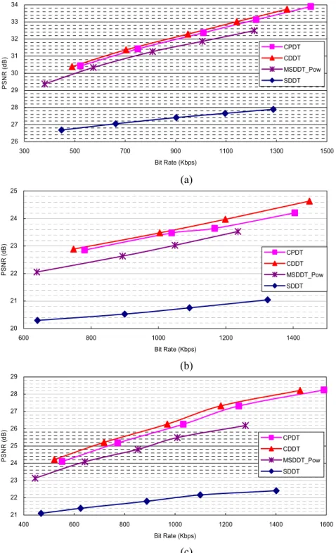
(10) Fig. 18. MSE vs. bit rate when running MSDDT with various α, and R combinations for Akiyo (upper left), Foreman (upper right), Mobile (lower left), and Stefan (lower right) at 2048-Kbps BL bit rate .............................................................................37 Fig. 19. αopt vs. bit rate for Akiyo (upper left), Foreman (upper right), Mobile (lower left), and Stefan (lower right) at 256-Kbps BL bit rate ..................................................38 Fig. 20. αopt vs. bit rate for Akiyo (upper left), Foreman (upper right), Mobile (lower left), and Stefan (lower right) at 512-Kbps BL bit rate ..................................................38 Fig. 21. αopt vs. bit rate for Akiyo (upper left), Foreman (upper right), Mobile (lower left), and Stefan (lower right) at 1024-Kbps BL bit rate ................................................39 Fig. 22. αopt vs. bit rate for Akiyo (upper left), Foreman (upper right), Mobile (lower left), and Stefan (lower right) at 2048-Kbps BL bit rate ................................................39 Fig. 23. The fitting curve for (R, αopt) using the power-law model ...................................40 Fig. 24. FGS-to-MPEG-1 transcoding performance comparison under FGS base-layer bit rate of 256 Kbps. (a) Foreman (b) Mobile (c) Stefan............................................43 Fig. 25. FGS-to-MPEG-1 transcoding performance comparison under FGS base-layer bit rate of 512 Kbps. (a) Foreman (b) Mobile (c) Stefan............................................44 Fig. 26. FGS-to-MPEG-1 transcoding performance comparison under FGS base-layer bit rate of 1024 Kbps. (a) Foreman (b) Mobile (c) Stefan..........................................45 Fig. 27. FGS-to-MPEG-1 transcoding performance comparison under FGS base-layer bit rate of 2048 Kbps. (a) Foreman (b) Mobile (c) Stefan..........................................46 Fig. 28. FGS-to-MPEG-2@MP transcoding performance comparison under FGS base-layer bit rate of 256 Kbps (a) Akiyo (b) Foreman (c) Mobile (d) Stefan ......50 Fig. 29. FGS-to-MPEG-2@MP transcoding performance comparison under FGS base-layer bit rate of 512 Kbps (a) Akiyo (b) Foreman (c) Mobile (d) Stefan ......52 Fig. 30. FGS-to-MPEG-2@MP transcoding performance comparison under FGS base-layer bit rate of 1024 Kbps (a) Akiyo (b) Foreman (c) Mobile (d) Stefan ....54 Fig. 31. FGS-to-MPEG-2@MP transcoding performance comparison under FGS base-layer bit rate of 2048 Kbps (a) Akiyo (b) Foreman (c) Mobile (d) Stefan ....56 Fig. 32. FGS-to-MPEG-4@SP transcoding performance comparison under FGS base-layer bit rate of 256 Kbps (a) Akiyo (b) Foreman (c) Mobile (d) Stefan ......58 x.

(11) Fig. 33. FGS-to-MPEG-4@SP transcoding performance comparison under FGS base-layer bit rate of 512 Kbps (a) Akiyo (b) Foreman (c) Mobile (d) Stefan ......60 Fig. 34. FGS-to-MPEG-4@SP transcoding performance comparison under FGS base-layer bit rate of 1024 Kbps (a) Akiyo (b) Foreman (c) Mobile (d) Stefan ....62 Fig. 35. FGS-to-MPEG-4@SP transcoding performance comparison under FGS base-layer bit rate of 2048 Kbps (a) Akiyo (b) Foreman (c) Mobile (d) Stefan ....64 Fig. 36. Estimated operational complexity comparison of the six transcoding architectures for Foreman .....................................................................................70. xi.

(12) List of Notations Â. DCT-domain representation of signal A. P. Motion compensated 8×8 block. Q. Reference 8×8 block. H, G. Translation matrix. MC(i)(.). Motion compensation at decoder/encoder loops. IQ(.), Q(.) Inverse quantization and quantization Xn. The decoded frame at decoder-loop at time instance n. X*n. The reconstructed frame at encoder-loop at time instance n. Yn. The reconstructed frame at decoder-loop at time instance n. ∆Xn. The residue at the encoder-loop at time instance n. Bn. The base-layer residue coefficient at time instance n. En. The enhancement-layer coefficient at time instance n. mv(i). Motion vector at decoder/encoder loops. S(.). Saturation. D. Drift error. dp. Incoherent error. dq. Arithmetic error. RE. The original enhancement-layer bit rate. Rε. The error-layer bit rate. α. The ratio of the original enhancement layer in the enhancement layers. αopt. The rate-distortion optimized α. D(.). Distortion function. R. Bit rate for both enhancement layers. IC. Total instruction counts. B. xii.

(13) Φ. Workload percentage of modules in transcoder. xiii.

(14) Chapter 1 Introduction In this chapter, we will briefly introduce the role that video transcoding plays in the framework of MPEG-21 Universal Multimedia Access. The scope of this thesis is also presented as a concluding remark.. 1.1. Overview of MPEG-21 Transcoding Systems In recent years, the popularity of internet has boosted the need for efficient transmission of digital content. MPEG-21 provides a unified solution, Universal Multimedia Access (UMA) [1], to construct a multimedia content delivery and rights management framework. The primary concept of UMA is that any media resources should be available to any users at anytime and anywhere. However, the diversity of channel conditions and end-user capacities makes it a challenging task. It is inevitable that many types of conversions should be performed as an intermediate interface between server and terminal to accommodate different network constraints. Video transcoding is a technique of transforming a pre-compressed video bitstream from one format into another according to various network conditions and client devices. As shown in Fig. 1, the context format is referred to as coding parameters such as the bit rate, frame rate, spatial resolution, and coding syntax. One of the scenarios is a video conferencing system on the internet where the participants may use different terminals. Under this circumstance, a video transcoder (located at the transmitter, receiver, or somewhere in the network) is needed for both dynamically adjusting the bit rate in adaptation to each user’s available bandwidth and providing conversion across different 1.

(15) standards to enable content exchange. Hence, as media resources and communication networks expand in heterogeneity, video transcoding is one of the essential components for current and future multimedia systems to achieve inter-compatibility between different platforms.. Fig. 1. Video transcoding operations. 1.2. Scope of This Thesis Various transcoding algorithms provide trade-off between the computational complexity and reconstructed video quality [3]-[11]. In all, the most straightforward approach of realizing transcoding functionality is to cascade a decoder and an encoder, as shown in Fig. 2. The decoder decodes the original input video, and the encoder re-encodes the decoded data subject to any new constraints. Such a cascaded transcoding architecture which fully decodes the bitstream and re-encodes the video is treated as one of the most complicated methods and is very much computationally intensive. In this thesis, we aim to introduce more efficient techniques to balance the perceptual quality and the computational complexity.. Fig. 2. Cascaded decoder and encoder transcoder. Based on the concepts of UMA, we build a simplified UMA model on the internet. In this framework, the source video material is encoded and archived as MPEG-4 Fine 2.

(16) Granularity Scalable (FGS) bitstreams. In order to provide access to FGS coded bitstreams with both FGS enabled devices and devices that only support single-layer coding standards, a novel transcoder is proposed and implemented to convert the bitstream from FGS format to other single-layer video formats including MPEG-4 Simple Profile (SP), MPEG-2, and MPEG-1. Depending on the terminal capability, the universal transcoder is capable of supporting video contents of different formats. The remainder of this thesis is organized as follows. Chapter 2 classifies various transcoding architectures and discusses the fundamental problems. In Chapter 3, a framework for FGS to single-layer transcoding is introduced. Chapter 4 proposes the drift compensation architecture. Experimental results and analysis are presented in Chapter 5. Finally, Chapter 6 gives the concluding remarks.. 3.

(17) Chapter 2 State of the Art In this chapter, we will explore the prior arts on homogeneous (with similar standard) and heterogeneous (between different standards) video transcoding. An overview of transcoding architectures and techniques is provided along with an evaluation and discussion.. 2.1. Transcoding Architectures Efficient and effective transcoding architectures are needed to expand the applications of multimedia information exchange. As mentioned in the previous chapter, it is always possible to use a cascaded approach to perform transcoding. However the cost is too high to be feasible. The following subsections introduce several transcoding architectures that aim to reduce the computational complexity of the straightforward decoder-encoder implementation. The rationale behind these transcoding architectures is to reuse existed coding parameters or statistics from the input video bitstream. They may be applied not only to simplify the computation, but also to maintain or even improve the visual quality.. 2.1.1. Spatial-Domain Video Transcoding Fig. 3 illustrates the Cascaded Pixel-Domain Transcoder (CPDT) [3], which is very similar to the brute-force method. It is a concatenation of a standard decoder and a simplified encoder. The encoder does not perform full-scale motion estimation (ME). 4.

(18) Instead, it reuses the motion vectors as well as other information extracted from the input video bitstream. It is shown in [12] that the macroblock mode decision and ME module occupy about 70% of the overall encoder processing power. Hence, by avoiding these computationally intensive operations, it can speed up the transcoding process by roughly three times. Input Bitstream. Q1-1. VLD. IDCT. MV. MC. Frame Buffer. MV Mapping. Output Bitstream. VLC. Q2. +. DCT. − Q2-1. IDCT. Frame Buffer. MC. Fig. 3. Cascaded Pixel-Domain Transcoder (CPDT). The prior works based on CPDT architecture focus on the improvement of new motion vector (MV) information in the encoder-loop. Generally, a homogeneous transcoder which is designed for bit rate adaptation requires no MV mapping operation. The functional unit of MV Mapping presented in CPDT is used particularly for transcoding which involves spatial resolution adjustment or heterogeneous format change. However, since reduced resolution transcoding is beyond the scope of this thesis, we will focus our attention to the problem of changes in the directionality of MVs in heterogeneous transcoding. For instance, in the MPEG-4 standard [2], an inter-coded macroblock comprises either one MV for the complete macroblock or four MVs, one for 5.

(19) each non-transparent 8×8 pel blocks forming the 16×16 pel macroblock, whereas MPEG-1/2 support only 16×16 prediction in progressive frames. For transcoding bitstreams from MPEG-4 format into MPEG-1/2 format, problems arise when passing MVs directly from the decoder to the encoder. Fig. 4 shows the way of multiple MVs being merged to a single MV when the coding mode is different. Hence, a motion vector mapping operation is required. A variety of methods have been discussed for deriving a new MV from the four MVs available in the input bitstream information. Although these methods are originally developed for reduced resolution transcoding, they are also applicable in our scenario. One strategy is to select one of the incoming MVs in random [14]. Weighted average taking into account the prediction error is presented in [13]. Some other methods, such as median, majority, and average, are presented and compared in [12]. To further improve the accuracy for prediction, MV refinement is performed in a small search window around the composite MV [15]. Other issues related to heterogeneous transcoding, such as picture type conversion [12] or frame rate reduction [15]-[17], will not be mentioned later due to out of thesis scope.. Fig. 4. Motion vector composition. CPDT is usually considered to be free of drift error, and used as the benchmark for evaluating the performance. Although the reconstructed frames in the decoder-loop and the encoder-loop don’t match due to heterogeneous quantization table and other parameters, this CPDT will not introduce drifting error theoretically. The reason is that the encoder-loop will reconstruct the new coding residues to avoid the improper MV causing unexpected reconstruction mismatch. In addition, this CPDT is also flexible in 6.

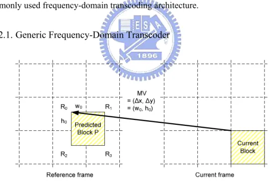
(20) coding-parameter changes. Because the decoder-loop and the encoder-loop separate from each other, more flexibilities are allowed to operate the transcoded video at different bit rates, frame rates, picture resolutions, coding modes, and even different standards.. 2.1.2. Frequency-Domain Video Transcoding The frequency-domain based video transcoding operates the video decoding and re-encoding in the transform domain. In contrast to the spatial-domain transcoding which operates the video transcoding in the spatial domain, the frequency-domain (or called transform-domain) transcoding architecture avoids three unnecessary transformations (one backward transform in the decoder-loop and one forward/backward transform in the encoder-loop) to achieve equal coding efficiency with lower complexity. This subsection introduces the core techniques in frequency-domain transcoding and reviews two types of commonly used frequency-domain transcoding architecture.. 2.1.2.1. Generic Frequency-Domain Transcoder. Fig. 5. Source block extraction problem. Motion compensation in the DCT-domain (MC-DCT) is the core technique in frequency-domain transcoding architecture. It operates the motion compensation (MC) in DCT domain to reconstruct the video without converting to pixel domain. The related researches in MC-DCT can be found in prior works [9], [18]-[20]. The design idea of 7.

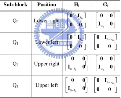
(21) MC-DCT is to build the relationship between the motion compensated 8×8 block (P) and the related reference blocks (Q). Since the MV (∆x, ∆y) usually is not 8×8 block aligned (see Fig. 5), the motion compensated block would cover at most four neighboring 8×8 blocks from the predicted MV center. The relationship in pixel domain is represented as eqn. (1). 3. P = ∑ H i Qi G i. (1). i= 0. where Hi and Gi are listed in Table 1. Ik represents an identity matrix of size k×k. The values of h0 and w0 are to be determined by the value of (∆x, ∆y) in MV (∆x, ∆y). Table 1. Matrices Hi and Gi. Sub-block. Position. Hi. Gi. Q0. Lower right. ⎡ 0 I h0 ⎤ ⎢ ⎥ ⎣0 0 ⎦. ⎡0 ⎢I ⎣ w0. Q1. Lower left. ⎡ 0 I h0 ⎤ ⎢ ⎥ ⎣0 0 ⎦. ⎡0 I 8− w0 ⎤ ⎢ ⎥ 0 ⎦ ⎣0. Q2. Upper right. ⎡ 0 ⎢I ⎣ 8− h0. 0⎤ 0 ⎥⎦. ⎡0 ⎢I ⎣ w0. Q3. Upper left. ⎡ 0 ⎢I ⎣ 8− h0. 0⎤ 0 ⎥⎦. ⎡ 0 I 8− w0 ⎤ ⎢ ⎥ 0 ⎦ ⎣0. 0⎤ 0 ⎥⎦. 0⎤ 0 ⎥⎦. From eqn. (1), the motion compensated block P consists of the lower-right part of sub-block Q0, the lower-left part of Q1, the upper-right part of Q2, and the upper-left part of Q3. Each component is computed by the pre-multiplication of Hi, which shifts the sub-block of interest vertically, and the post-multiplication of Gi, which shifts the sub-block horizontally. Since the DCT is a unitary orthonormal transform, it is distributive to matrix multiplication. Hence, we can express the DCT representation of eqn. (1) as 8.

(22) 3. ˆ ˆ ˆ Q Pˆ = ∑ H i iG i. (2). i= 0. where the 2D-DCT of an 8×8 block A is represented as Â = DCT(A). The horizontal and vertical displacement matrices can be pre-computed and stored in memory. In eqn. (2), the extraction of a single 8×8 block requires up to 4 × 8 × 64 × 2 = 4096 floating-point multiplications, which are huge computations. To speed-up the MC-DCT in [18], several faster implementations are proposed to improve the computation of eqn. (2). In [19], MC-DCT is simplified through factorizing the displacement matrices into relatively sparse matrices such that the number of computations required is reduced. The work in [9] approximates the elements of Ĥi and Ĝi to binary numbers and replaces the multiplication with shifters and adders. Another efficient computation method on macroblock basis is derived in [20]. It utilizes shared information within a macroblock, such as MV and common blocks, to yield substantial speedup in computation. The generic frequency-domain transcoder is constructed with the MC-DCT technique to allow entire transcoding operations in the frequency domain. Since MC can be performed in the frequency domain, the operations of DCT and IDCT in Fig. 3 can be saved to allow a structurally more efficient transcoding. Fig. 6 shows the design flow of the Cascaded DCT-Domain Transcoder (CDDT) proposed in work [6], which operates the transcoding without any DCT transformations in the frequency domain. There are two design issues in the generic frequency-domain transcoding architecture. The first is that MC-DCT may introduce reconstruction mismatches to cause transcoding drift error. Ideally, CDDT is a functionally equivalent representation of CPDT which is drift-free. However, the matrix multiplications in MC-DCT may introduce operational precision mismatches, and frame reconstruction in the frequency domain may introduce rounding errors. Although theses mismatches may cause drift, this type of transcoding error only leads to slight quality degradation and is almost ignorable. The second design issue is the operational complexity of the MC-DCT. The complexity of CDDT highly depends on the MC-DCT implementation method, and the complexity of MC-DCT depends on the complexity of matrix multiplication. Thus, applying an efficient. 9.

(23) matrix multiplication in MC-DCT can highly improve the frequency-domain transcoding efficiency.. Fig. 6. Cascaded DCT-Domain Transcoder (CDDT). 2.1.2.2. Simplified Frequency-Domain Transcoder More complexity reduction can be achieved by analyzing and improving the redundancy in CDDT. For real-time applications, the complexity in CDDT is still too high to be used. To analyze the CDDT as shown in Fig. 6, we find the behavior of the frame reconstruction in the decoder-loop and the encoder-loop is almost identical under the assumption of the same MC behavior and the same quantization step size. The MC behavior depends on video encoding standards and will not be an issue if both the decoder-loop and encoder-loop specify the same MC structure. The quantization step size is controlled by many encoding parameters such as the rate control. Therefore, to simplify the CDDT architecture, the two frame reconstruction operations should be merged by using a shared MC to compensate for the quantization mismatches between the decoder-loop and the encoder-loop. Such an idea can be easily realized in homogeneous 10.

(24) transcoding which uses the same MC structure. Some prior works in [7]-[9] design their simplified transcoders based on such a design idea to save one more MC operation. To identify the design idea, a brief derivation is provided as follows. From Fig. 6, the residual in the encoder-loop is given by. + X n = X n − MC (. 2). (X. * n −1. , mv(. 2). ). (3). where MC(.) is the motion compensation process, the subscript on the variable indicates time, and the superscript of “1” and “2” represents the decoder-loop and the encoder-loop, respectively. Here, we denote a signal with quantization effect as X * = IQ ( Q ( X ) ). (4). where Q(.) and IQ(.) stand for quantization and inverse quantization, respectively. The reconstructed signal in the decoder-loop is given by. (. X n = Bn + MC (1) Yn −1 , mv(1). ). (5). Substituting eqn. (5) into eqn. (3), we can yield. (. ). + X n = Bn + MC ( ) Yn −1 , mv( ) − MC ( 1. 1. 2). (X. * n −1. , mv(. 2). ). (6). Assuming mv(1) = mv(2) (i.e., MVs are not recalculated) and the sub-pixel MCs in the decoder-loop and encoder-loop perform the same interpolation filtering, it can be stated that. (. ). (. MC (1) X n , mv(1) = MC ( 2) X n , mv ( 2). ). (7). Based on the assumption that the MC is a linear operation, i.e., MC(X + Y, mv) = MC(X, mv) + MC(Y, mv), we may rewrite eqn. (6) as. (. + X n = Bn + MC Yn −1 − X n*−1 , mv( ) 1. ). (8). From eqn. (8), the prediction residual in the encode-loop in the transcoder can be obtained by adding the motion compensated frame differences to the incoming prediction residual. 11.

(25) Since Yn = Xn, we have. (. + X n = Bn + MC X n −1 − X n*−1 , mv( ) 1. ). (9). Furthermore, we may get the corresponding equivalent equation for Xn-1 – X*n-1 by applying eqn. (3).. (. ). X n −1 − X n*−1 =+ X n −1 + MC X n*− 2 , mv (1) − X n*−1. ( −(X. ( − MC ( X. )) , mv ( ) ) ). =+ X n −1 − X n*−1 − MC X n*− 2 , mv (1) =+ X n −1. n −1. * n−2. 1. *. (10). =+ X n −1 −+ X n*−1 Finally, eqn. (9) is reduced to. (. + X n = Bn + MC + X n −1 −+ X n*−1 , mv( ) 1. ). (11). Based on eqn. (11), the architecture in Fig. 6 is transformed into the architecture in Fig. 7. This is referred to as the Simplified DCT-Domain Transcoder (SDDT). Significant complexity reduction is attained in SDDT. Compared to CPDT in Fig. 3, SDDT not only eliminates the DCT/IDCT, but also reduces the size requirement of frame buffers by half. Only one MC loop is required to store the difference values between the reconstructed pictures in the decoder-loop and the encoder-loop in this architecture. This complexity reduction is achieved in sacrifice of the flexibility of cascaded architectures. In the above derivation, SDDT assumes the MVs after the transcoding to be the same as those before the transcoding in order to merge the two MCs. This architecture is based on the assumption of using the same MC structure, so SDDT has limited applications such as bit rate transcoding.. 12.

(26) Fig. 7. Simplified DCT-Domain Transcoder (SDDT). Fig. 8. Open-loop transcoder. 2.2. Video Transcoding Techniques The video transcoding techniques are built upon the transcoding architectures presented in Section 2.1, and used to improve the transcoding performance by adjusting the encoding parameters. Two common transcoding techniques including intra refreshment and rate control are reviewed.. 2.2.1. Intra-Refresh Technique To stop the drift propagation of errors introduced in reduced resolution transcoding, an intra-refresh transcoding technique is proposed in [10]. The intra-refresh technique adaptively forces the inter-coded blocks to be intra-coded based on drift estimation in the compressed bitstream. Since intra-coded blocks will not use the other frames for image reconstruction, this type of conversion stops the drift propagation.. 13.

(27) Fig. 9. Intra refresh in open-loop architecture. Fig. 9 shows an open-loop transcoder in which the intra-refresh technique is applied. The module Inter-to-Intra Conversion in Fig. 9 either bypasses the inverse quantized DCT coefficients or uses the reconstructed coefficients from the frame memory instead according to the intra-refresh rate, which is the percentage of intra-coded macroblocks in one frame. The intra-refresh rate is adaptively adjusted according to the estimated value of drift. It should be noted that more bits are usually required for coding intrablocks. Therefore, the intra-refresh operation and the rate control must be considered jointly. Although the intra-refresh technique demonstrates the ability to correct drift errors, its effectiveness is achieved using additional MC and frame memory to reconstruct the reference frame for the inter-to-intra conversions of the DCT coefficients. The architecture in Fig. 9 may seem to require less memory and computation than CPDT and CDDT. The reason is that the open-loop transcoder upon which the intra-refresh technique is implemented needs no MC prediction loop at all. If the intrablock refresh method is realized in close-loop architectures [11], the question whether complexity reduction is possible remains debatable.. 14.

(28) 2.2.2. Rate Control Issues The purpose of rate control is to provide better and consistent video quality under the bandwidth constraint. It involves two basic steps, picture-layer bit allocation and macroblock-layer rate control. The picture-layer bit allocation determines the target bit budget for each frame. The macroblock-layer rate control adjusts the quantization parameters for coding the macroblocks. Generally speaking, all rate-control algorithms designed for video coding are applicable to transcoding. Rate control in transcoding either targets at providing accurate bit rate adaptation or improving the coding efficiency by exploiting the coding statistics collected from the input compressed bitstream. The design issue for bit rate transcoding is actually the same as that for conventional video coding. It is to allocate proper bits to a picture proportional to its complexity such that the output rate would comply with the bit rate constraint. The only difference lies in the availability of content characteristics for transcoding. A straightforward implementation for bit rate transcoding might scale the input bits of each frame, which can be easily obtained from the pre-encoded video streams, according to the rate conversion ratio. Better bit allocation is possible by further exploiting the correlations between the input and the output picture complexities [21]. In [22], a ρ-domain rate-distortion model is adopted to obtain the optimal number of bits for each frame. This frame-level rate-distortion information is pre-generated in the front-encoder and transmitted to the transcoder as side information. The work in [9] derives the optimal set of quantizer scales based on Lagrangian optimization.. 2.3. Evaluation of Transcoding Architectures In the previous sections, we have discussed the transcoding architectures and transcoding techniques. Each architecture raises different design trade-off issue in computational complexity and visual quality. This section analyzes these transcoding architectures in terms of complexity and drift error.. 15.

(29) 2.3.1. Complexity Analysis Table 2 shows the complexity analysis for four types of transcoding architecture. The first type referred to as DEC-ENC implements a straightforward method to fully decode the input bitstream and fully encode the reconstructed video from the decoder side. Such a method doesn’t save any computations and is the most computationally intensive. It needs 1 ME, 3 DCT/IDCT, and 2 MC operations. Type II implements CPDT architecture which reconstructs the video in pixel domain. Such a method saves 1 ME compared to Type I. Type III implements CDDT architecture which is a generic DCT-domain transcoder. This type of architecture saves 3 more DCT/IDCT operations compared to Type II. Type IV shows the most competitive ability in computational complexity compared to the first three types. It implements the simplified CDDT (also referred to as SDDT) which saves 1 more MC operation and 1 more frame buffer compared to Type III. From the viewpoint of computational complexity, Type I suffers most efforts in transcoding and Type IV is the most computationally efficient architecture which has more than 50% of computation reduction. Table 2. Complexity analysis of four transcoding architectures. Type. Transcoding. ME Frame DCT/. Architecture. Buffer IDCT. MC Spatial. Transform. I. DEC-ENC. 1. 2. 3. 2. 0. II. CPDT. 0. 2. 3. 2. 0. III. CDDT. 0. 2. 0. 0. 2. IV. SDDT. 0. 1. 0. 0. 1. 2.3.2. Drift Error Analysis Drift errors come from imperfect frame reconstruction during transcoding procedure, and the imperfect frame reconstruction causes the mismatches to propagate between frames. Analyzing the four architectures in Table 2, the mismatches come from two major sources. The first type of mismatch comes from arithmetic operations 16.

(30) including rounding errors or precision conversion errors, and is also referred to as arithmetic error in this thesis. We have identified three possible sources for the arithmetic error. The first source of error relates to the floating-point operation in transcoding. For example, different from pixel-domain MC, DCT-domain MC reconstructs the video in the DCT domain through floating-point matrix multiplication. But no processor can provide infinite precision to accurately manipulate these numeric data. Mismatch is then introduced. The second and third sources of error are due to the failed linearity assumption on which the derivation of SDDT is based, and hence are unique to SDDT. In the derivation of SDDT, in order to merge the MC operations in the decoder-loop and encoder-loop, we have assumed that MC is a linear operation which is not strictly true in practical situations. The second source of error comes from the saturation after the MC operation. In most standard video encoders, a clipping function is required in front of the frame memory. It saturates the reconstructed pixel values to lie in the range [0:255]. Taking into account the saturation, we can not reduce eqn. (6) into eqn. (8).. ( ) , mv ). + X n = Bn + MC ( S (Yn −1 ) , mv ) − MC S ( X n*−1 ) , mv. (. ≠ Bn + MC S (Yn −1 − X n*−1. ). (12). where S(.) denotes the saturation. In eqn. (12), the inequality is due to the nonlinear property of the clipping operation. Thus, combining the two frame memories in the derivation is inaccurate and the resultant architecture can produce errors. The third source of error comes from the rounding operations in MC. When the MV is in half-pixel precision, the MC calculates the half-samples by simple linear interpolation from the neighboring actual samples. The interpolation performs a rounding operation to obtain the closest integer. In CPDT and CDDT, the rounding function is applied to the reconstructed coefficients in the decoder-loop and encoder-loop, respectively. However, in SDDT, it is carried out with the differences. It can be shown that this mismatch might introduce error.. 17.

(31) Let a, b be the values after half-pixel MC in the decoder-loop and the encoder-loop in CDDT, respectively. For simplicity, consider only horizontal component of the MV consists of half-pixel precision, then ⎛ Y ( i, j ) + Yn −1 ( i + 1, j ) ⎞ a = round ⎜ n −1 ⎟ 2 ⎠ ⎝ ⎛ X * ( i, j ) + X n*−1 ( i + 1, j ) ⎞ b = round ⎜ n −1 ⎟ 2 ⎝ ⎠. (13). where i, j denote the horizontal and vertical coordinates, respectively. The difference signal should be ⎛ X n*−1 ( i, j ) + X n*−1 ( i + 1, j ) ⎞ ⎛ Y ( i, j ) + Yn −1 ( i + 1, j ) ⎞ − a − b = round ⎜ n −1 round ⎜ ⎟ ⎟ 2 2 ⎝ ⎠ ⎝ ⎠. (14). However, the value after the same half-pixel MC in SDDT would be ⎛ (Yn −1 ( i, j ) − X n*−1 ( i, j ) ) + (Yn −1 ( i + 1, j ) − X n*−1 ( i + 1, j ) ) ⎞ ⎟ c = round ⎜ ⎜ ⎟ 2 ⎝ ⎠. (15). In general, a – b ≠ c. Therefore, the rounding function in sub-pixel MC causes error. Table 3. Different types of drift error. Drift Error Type. Arithmetic error. Incoherent error. Sources. Architectures Affected. Floating-point arithmetic. CDDT, SDDT. Saturation in MC. SDDT. Rounding in MC. SDDT. Incoherent MC structure. SDDT. The second type of mismatch comes from incoherent frame reconstruction. Since the decoder-loop and encoder-loop of the transcoder may come from two different compression standards, the MC structure may use different reconstruction procedure which causes the reconstruction mismatch. One example is the MPEG-4 to MPEG-2 transcoding in which MPEG-4 supports four MVs but MPEG-2 doesn’t. Such a mismatch. 18.

(32) is referred to as incoherent error in this thesis. The above discussion is summarized in Table 3. Table 4 shows the drift error analysis of the four transcoding architectures. Type I and Type II reconstructs the video in pixel domain which is a standard compliant flow, so no drift error is involved. Type III which operates the MC in the DCT domain suffers from the first type of mismatch in rounding errors and precision conversion errors. Type IV which saves one more MC compared to Type III suffers from the same mismatch as Type III, but it introduces another mismatch in incoherent errors. The preserved single MC only implements the quantization error compensation. If heterogeneous transcoding which involves incoherent MC structures is implemented, such a type of transcoding architecture has no ability to compensate for these incoherent errors. Compared to the arithmetic error, the incoherent error leads to more serious quality degradation in transcoding. Table 4. Drift error analysis of four transcoding architectures. Type. Transcoding. Types of Drift. Error Effects. Architecture. I. DEC-ENC. N/A. N/A. II. CPDT. N/A. N/A. III. CDDT. Arithmetic errors. Minor. IV. SDDT. Arithmetic errors. Minor for coherent MC structure. +. Medium to serious for incoherent MC. Incoherent errors. structure. 2.3.3. Evaluation and Discussion A new design challenge is raised in striking the balance between computational complexity and drift error reduction. From Table 2 and Table 4, Type I and II have the highest computational complexity, but introduce no drift errors. Type III has the medium complexity, but suffers from minor drift errors. Type IV has the lowest complexity, but 19.

(33) introduces minor drift errors in coherent MC structure and medium to high drift errors in incoherent MC structure. For real-time applications, we need the Type III’s drift error performance and Type IV’s computational complexity. In this thesis, we will explore another possibility to construct a multi-layer to single-layer transcoding architecture based on Type IV, but compensate for the drift errors by introducing the multi-layer transcoding technique.. 20.

(34) Chapter 3 FGS to Single-Layer Transcoder In this thesis, we focus on building a transcoding framework for FGS to single-layer transcoding. The multi-layer to single-layer transcoding framework is constructed on the basis of simplified frequency-domain transcoding architecture (SDDT) which is a single-layer to single-layer transcoding architecture. We extend this SDDT architecture to be used in multi-layer to single-layer transcoding such as FGS-to-MPEG-1/2/4. The design issues raised in homogeneous and heterogeneous transcoding are also discussed.. 3.1. Multi-Layer to Single-Layer Transcoding Framework The proposed transcoding framework targets on using a unified structure for converting MPEG-4 FGS multi-layer bitstream to MPEG-1/2/4 single-layer bitstream. For real-time application which needs least computation, the SDDT with least transcoding computation compared to the other spatial or frequency domain transcoding architectures is adopted in this thesis. Since the SDDT is a single-layer to single-layer transcoding architecture, it can not be applied directly to our target application of FGS-to-MPEG-1/2/4 transcoding which is a multi-layer to single-layer transcoding. Some modifications are needed to allow the SDDT architecture to be applied to our FGS-to-MPEG-1/2/4 transcoding framework.. 21.

(35) Fig. 10. FGS to single-layer CDDT. The proposed multi-layer to single-layer transcoding framework is to integrate the SDDT. with. a. FGS-to-single-layer. transcoder.. In. previous. days,. many. FGS-to-single-layer transcoding works have been proposed. The authors in [24] proposed a single MC architecture in the spatial domain for FGS-to-MPEG-4@SP transcoding. Following a likewise work, we are able to integrate the SDDT with work [24] to extend the SDDT functionality to be compatible with FGS scalability. To provide a clear description about our multi-layer to single-layer transcoding framework, Fig. 10 first shows the design flow chart for FGS-to-single-layer CDDT and then follows the step-by-step derivation to FGS-to-single-layer SDDT as shown in Fig. 11. In the beginning, the decoder-loop in the transcoder receives two FGS coded bitstreams including a base layer (BL) and an enhancement layer (EL). The reconstructed picture in the decoder-loop is given by. (. Yn = Bn + MC ( ) Yn −1 , mv( ) 1. 22. 1. ). (16).

(36) It should be noted that the EL is independent of the MC in the BL, and directly added to the reconstructed coefficients after being bit-plane decoded.. X n = Yn + En. (17). Substituting eqns. (16) and (17) into eqn. (3), we may obtain + X n = X n − MC (. 2). (X. * n −1. = (Yn + En ) − MC (. (. , mv (. 2). (X. (. ). 2). * n −1. , mv(. ). 2). ). ). (18). = Bn + MC ( ) Yn −1 , mv ( ) + En − MC ( 1. 1. 2). (X. * n −1. , mv (. 2). ). Assuming mv(1) = mv(2), MC(1)(X, mv) = MC(2)(X, mv), and MC is a linear assumption, we can derive eqn. (19) from eqn. (18).. (. ). + X n = Bn + MC Yn −1 − X n*−1 , mv(1) + En. (19). Applying eqn. (17) into eqn. (19), we can yield. ( + MC ( ( X. ). + X n = Bn + MC Yn −1 − X n*−1 , mv ( ) + En = Bn. 1. ). () * + En n −1 − En −1 ) − X n −1 , mv 1. (20). Replacing the frame differences with the residual differences as in eqn. (10), eqn. (20) is reduced to. (( X = B + MC ( ( + X. + X n = Bn + MC n. ). − X n*−1 ) − En −1 , mv ( ) + En 1. n −1. ). () * + En n −1 −+ X n −1 ) − En −1 , mv 1. (21). This derivation for prediction residual as shown in eqn. (21) is very similar to eqn. (11) which we have in SDDT, except for those enhancement-layer related terms. The influence of the EL is in two ways. Firstly, the reconstructed frame as shown in eqn. (17) contains the EL coefficients (En) for refinement. Secondly, the reconstructed frame with EL refinement is used to reconstruct the next reference frame for the encoder-loop which originally should use BL only to reconstruct pictures. The second influence will introduce mismatches for those using the decoded set of MVs and residues without proper 23.

(37) correction. Different reconstructed frames are generated between the transcoder and end-users, and such a mismatch will propagate frame by frame with obvious quality degradation. To avoid the mismatches, the effects of EL in reconstructed frames must be removed. One possible solution is to implement a full-scale ME for the correct MVs to be used for the reconstruction from BL added with EL. But such a solution costs too much computation. Another way is to remove the effects of EL from the reconstructed frames in the encoder-loop. Therefore, the term of En-1 in eqn. (21) is added to avoid the reconstruction mismatches between the transcoder and end-users. The proposed multi-layer to single-layer transcoding framework is shown in Fig. 11. Based on this framework, we are able to transcode the FGS bitstream to either format of MPEG-1/2/4 video bitstream by merely replacing the standard compliant entropy coder (VLC), quantization table (Q2), etc.. Fig. 11. FGS to single-layer transcoder. The multi-layer to single-layer transcoding framework preserves the same transcoding efficiency as the SDDT in computation. Compared to the CDDT shown in Fig. 10, the proposed framework saves 1 MC operation and 1 frame memory, and 4 more DCT/IDCT as compared to the CPDT. Although the proposed multi-layer to single-layer transcoding framework is a computationally efficient architecture, it suffers from the same problems as the SDDT including arithmetic error and incoherent error which are mentioned in Chapter 2. To dig 24.

(38) deeper to see the problems, we have identified three possible sources to cause drift errors in the proposed framework. 1.. Rounding mismatches and precision conversion mismatches from MC-DCT.. 2.. Rounding mismatches and saturation mismatches from single MC implementation in frequency domain.. 3.. Incoherent errors from heterogeneous transcoding.. The effects for the first and second types are minor and usually negligible. The third type which is dedicated to the heterogeneous transcoding has dominant influences on drift errors if the drift errors are not well-handled. In the next section, we will dedicate the discussion to the design issues of heterogeneous transcoding.. 3.2. Design Issues of Heterogeneous Transcoding This section discusses the design issues to explore the exact drift error sources in heterogeneous transcoding. As what we have discussed, the proposed framework has three possible drift error sources. The first type including rounding mismatch and precision conversion mismatch is dedicated to the MC-DCT problems. The matrix operations in MC-DCT determine how serious this problem will be. For example, the matrix operational results using integer precision representation is different from using double precision representation. But, usually such a mismatch contributes minor drift errors and is ignorable. The second type including rounding mismatch and saturation mismatch is introduced by using single MC in the frequency domain. In eqn. (19), we have assumed. MC(Yn-1 – X*n-1, mv) =. MC(Yn-1, mv) – MC(X*n-1, mv) under the. assumption that MC(.) has the linear characteristic. But the sub-pixel interpolation operations in MC(.) contain rounding and saturation operations which are non-linear. Such a type of mismatch is similar to the first type which is one kind of arithmetic errors and will only introduce minor drift errors in general. The third type is the incoherent error from heterogeneous transcoding. This type of mismatch comes from the incompatible coding toolsets in various compression standards. To analyze this type of mismatch, we need to survey the supported toolsets in these standards we want to support. 25.

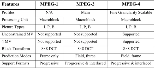
(39) Table 5. A summary of the toolsets in MPEG-1, MPEG-2, and MPEG-4. Features. MPEG-1. MPEG-2. MPEG-4. N/A. Main. Fine Granularity Scalable. Macroblock. Macroblock. Macroblock. I, P, B. I, P, B. I, P, B. Unconstrained MV. Not supported. Not supported. Supported. 4 MV. Not supported. Not supported. Supported. Block Transform. 8×8 DCT. 8×8 DCT. 8×8 DCT. Prediction Modes. Frame only. Field, frame. Field, frame. Support Formats. Progressive. Progressive & interlaced. Progressive & interlaced. Profiles Processing Unit Picture Types. Table 5 summaries the supported coding toolsets in MPEG-1, MPEG-2 and MPEG-4. From this table, we can observe that the coding toolsets supported by MPEG-1 and MPEG-2 are quite similar, except for the interlaced mode support, entropy coding tables and quantization tables, etc. MPEG-4 has more distinct differences in supported coding toolsets compared to MPEG-1/2. According to eqn. (19), what we really need to care is 4-MV and Unconstrained MV (UMV) which may fail our assumption of mv(1) = mv(2). Four MV is to support the MC on 8×8 block basis. Since MPEG-1/2 does not support MV for 8×8 block, we need to re-map these four 8×8 MVs into a new 16×16 MV for coding. The UMV is to allow MPEG-4 MV to point out of the picture boundary, while MPEG-1/2 doesn’t. To simplify the computation, only a simple clipping operation is used to limit the UMV to lie inside the picture boundary. Although the input MV can be modified to comply with the syntax in the end-decoder, it is not the correct MV for the corresponding prediction error. In two MC architectures such as CPDT and CDDT, the MC loop in the encoder-loop re-computes the prediction residual according to the re-mapped MV. However, the same design flow is not suitable for our multi-layer to single-layer transcoding framework, since in our multi-layer to single-layer framework, it doesn’t allow the residue re-compilation. So, the coding residues will not be able to match the motion compensated data for perfect reconstruction. And then, obvious quality degradation occurs. To solve this problem, we 26.

(40) derive a new equation for the prediction residual in the encoder-loop in the transcoder by taking into account these heterogeneous transcoding effects. From eqn. (18), we modify the eqn. (18) into eqn. (22) by removing the assumption of mv(1) = mv(2). ) ) ) ( X , mv( ) )) () , mv ( ) ) + E ) − MC ( ) ( X , mv ( ) ) ) + ( MC ( ) (Y , mv( ) ) − MC ( ) (Y , mv( ) )) = ( ( B + E ) + ( MC ( ) (Y , mv ( ) ) − MC ( ) ( X , mv ( ) ) ) ) + ( MC ( ) (Y , mv( ) ) − MC ( ) (Y , mv( ) )) = ( ( B + E ) + MC ( ) (Y − X , mv ( ) ) ) + ( MC ( ) (Y , mv ( ) ) − MC ( ) (Y. (( B + MC (Y = ( ( B + MC (Y. +Xn =. (1). n. , mv ( ) + En − MC ( 1. n −1. 1. 1. n −1. n. 2. 2. 2. 2. 2. * n −1. 2. 2. n −1. 2. 2. 2. 1. 1. 2. (22). 2. * n −1. n −1. n. 2. n −1. n −1. 2. n. * n −1. n. n −1. n. 2. 2. * n −1. n −1. n. 1. 1. 2. n −1. n −1. , mv (. 2). )). Note that the difference between eqns. (19) and (22) is in the second term which is the difference of using different MVs for MC. To integrate eqn. (10) into eqn. (22), we get a new form as eqn. (23).. (+ X −+ X MC ( ) (Y , mv ( ) ) − MC ( ) (Y. + X n = Bn + En + MC ( 1. 2). * n −1. n −1. 1. − En −1 , mv (. ( n −1 , mv. 2. n −1. ). 2). 2). )+. (23). In eqn. (23), the prediction error in the encoder-loop in a heterogeneous transcoder comprises the original decoded prediction error from the input bitstreams (including BL and EL) and an additional drift error term. The drift error (d) can be expressed as d = MC (. 2). (+ X. n −1. −+ X n*−1 − En −1 , mv(. 2). ) + MC ( ) (Y 1. n −1. ). , mv ( ) − MC ( 1. = dq + d p. 2). (Y. n −1. , mv (. 2). ). (24). where. d q = MC (. 2). (+ X. n −1. −+ X n*−1 − En −1 , mv(. and. 27. 2). ). (25).

(41) (. ). d p = MC ( ) Yn −1 , mv( ) − MC ( 1. 1. 2). (Y. n −1. , mv(. 2). ). (26). In eqn. (24), the drift error has been decomposed into two components. The first component dq represents the arithmetic error which we may neglect as mentioned in Section 3.1. This is a common drift error that has been observed in many other transcoding works. In Fig. 11, the motion-compensated loop is used to compensate for this type of error. The second component dp is from the heterogeneity of MC implementation between the decoder-loop and encoder-loop. Since MPEG-1/2 supports neither four MV MC nor unrestricted MC, the prediction residual of an inter-coded macroblock should be compensated with the differences between the predictions formed in the decoder-loop and encoder-loop. This type of error is also referred to as the incoherent error in Section 2.3.2. This incoherent error may cause more than 2 dB quality loss in PSNR depending on different GOP sizes or sequences. Targeting on drift-free transcoding, the two types of drift errors dq and dp where dp dominates how serious the drift errors in the proposed multi-layer to single-layer transcoding framework will be should be eliminated. The component dp is composed of the difference between the two MCs in the decoder-loop and the encoder-loop. For homogeneous transcoding, dp can be easily eliminated since MC(1)(.) = MC(2)(.) under the assumption of mv(1) = mv(2). But in heterogeneous transcoding with single MC architecture, the unknown property of mv(1) = mv(2) and MC(1)(.) = MC(2)(.) makes the dp unpredictable. First, mv(2) may come from various combinations in the cases of four MV or UMV. Secondly, since only one MC is used, we can’t predict both MC(1)(.) and MC(2)(.). Such two reasons make dp unable to be reconstructed perfectly theoretically. The prior arts adopt various transcoding techniques such as intra refreshment to stop the error propagation, but these methods only focus on eliminating the drift errors, but not stopping the error generation. To perfectly stop the error generation, we need side information to compensate for the dp. Therefore, in addition to the BL and EL, a third auxiliary layer is introduced in the transcoding design to compensate for the incoherent errors. Such a technique is called multi-layer transcoding technique in this thesis.. 28.

(42) Chapter 4 Multi-Layer Transcoding Approach In this chapter, a novel multi-layer transcoding approach is proposed to compensate for the drifting error from the incoherent MC structure. This multi-layer transcoding approach introduces an additional enhancement-layer (EL) bitstream containing the pre-calculated incoherent errors. This pre-calculated error layer is used to compensate for the errors in heterogeneous transcoding for the drift-free target. Under channel bandwidth limitation, a rate-distortion model is presented to optimize the streaming in original enhancement layer and this additional enhancement layer.. 4.1. Drift Compensation with Additional Enhancement Layer Severe drift error may be introduced in our multi-layer to single-layer transcoding framework when transcoding operates across different video compression standards. According to the analysis in Section 3.2, the reason is that the proposed SDDT architecture only compensated for the arithmetic errors which primarily come from the re-quantization process, but neglected the component of the incoherent errors, which comes from the incoherent MC structures between different standards. However, as what we demonstrated in Section 3.2, using single MC structure is unable to obtain enough information for drift-free heterogeneous transcoding. As shown in eqn. (26), the required information for compensating for the incoherent errors comes from the decoder-loop in the transcoder (Yn-1), which is not available in the multi-layer to single-layer transcoding framework with single MC. There were other drift-elimination schemes such as the intra refresh technique, but they all suffer from the weakness of inexact compensation. Such 29.

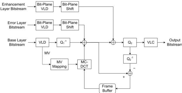
(43) kinds of transcoding techniques only stop the error propagation by periodically update an error-free block or an error-free frame passively. To aggressively solve this error drifting problem, the error information should be available for compensation. Therefore, to perform drift-free transcoding using the proposed multi-layer to single-layer framework which is unable to generate such an error term on its own, we need these error information to be transmitted from the front-encoder.. +. Bit-Plane Shift. DCT. −. Bit-Plane VLC. Error Layer Bitstream. MC + −. MV Mapping. Original Video. +. DCT. DCT. −. Bit-Plane Shift. Q1. Bit-Plane VLC. VLC. Enhanecment Layer Bitstream. Base Layer Bitstream. Q1-1. IDCT. Frame Buffer. MC. ME. Fig. 12. Corresponding FGS encoder framework for MSDDT. The multi-layer streaming technique is to pre-generate the incoherent errors dp in the font-encoder due to that this encoder is able to generate the same information as the decoder-loop in the transcoder. From eqn. (26), We can find that generating the mismatch due to different MC structures requires only the reference pictures in the decoder-loop in the transcoder, under the assumption of MC(1)(X, mv) = MC(2)(X, mv). Thus, we may 30.

(44) pre-generate the incoherent errors in the front-encoder as eqn. (27) and transmit the errors as side information to the transcoder.. (. ). (. d p = MC ( ) Yn −1 , mv( ) − MC ( ) Yn −1 , mv( 1. 1. 1. 2). ). (27). Here, we also assumed that the MV mapping method is known in the front-encoder, which is true since this FGS encoder is designed especially for our application. Fig. 12 shows the modified FGS front-encoder, in which an additional EL is introduced by bit-plane coding the differences between the motion compensated predictions from different MC structures of the decoder-loop and encoder-loop. In the following, we will denote this additional EL as the error layer or EL2. Transferring of the component dp in eqn. (27) to the front-encoder does not bear any burden, since the video content for transcoding is mostly encoded in advance such that no real-time constraint is imposed. With introducing this auxiliary layer as side information, we can simply compensate for the drift error dp by bit-plane decoding the error layer bitstream. Fig. 13 shows the multi-layer to single-layer transcoding framework with the multi-layer transcoding technique. This architecture is referred to as the Multi-layer Simplified DCT-Domain Transcoder (MSDDT) in this thesis. In this architecture, the transcoding efficiency of SDDT which requires only one frame store and one MC is preserved. But since a third layer is introduced, we will need the corresponding VLD module for decoding this auxiliary bitstream, in which the overhead produced on computation is negligible. Hence, the structural simplicity of the original transcoding design is preserved while both sources of drift error are perfectly compensated if the error layer is completely received. The sole trade-off is that the transmission of the error layer bitstream requires additional bandwidth.. 31.

(45) Enhancement Layer Bitstream. Bit-Plane VLD. Bit-Plane Shift. Error Layer Bitstream. Bit-Plane VLD. Bit-Plane Shift. Base Layer Bitstream. VLD. Q1-1. Q2. VLC. Output Bitstream. MV MV Mapping. Q2-1. MCDCT. − + Frame Buffer. Fig. 13. Multi-layer Simplified DCT-Domain Transcoder (MSDDT). In summary, we implemented the multi-layer transcoding approach based on the proposed multi-layer to single-layer transcoding framework to resolve the drift propagation problem in heterogeneous transcoding. In an ideal case with infinite bandwidth, this proposed architecture shown in Fig. 13 should be able to obtain the same rate-distortion performance as CDDT. This is because both types of drift error (dq and dp) can be perfectly compensated. But the available bandwidth is usually constrained in most practical applications, and hence raises the issue of how to allocate the limited bandwidth resources to both layers (EL and error layer) for efficient transmission. In the next section, an optimized model is constructed for the selection of the enhancement layer and the error layer.. 4.2. Multi-Layer Transcoding with R-D Optimization An R-D model is constructed to solve the multi-layer transcoding problems under the limited channel bandwidth. To perform drift-free transcoding, an additional error layer containing the coefficients of the incoherent errors is used as side information to be transmitted to the transcoder. But since channel bandwidth is limited, the resource. 32.

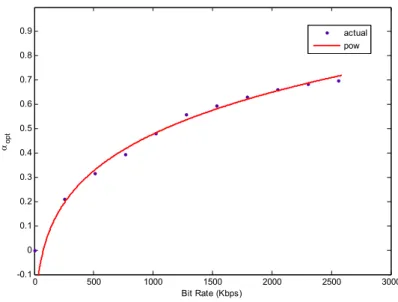
(46) allocation for achieving the best transcoding performance and decoded video quality becomes very important. To model the resource allocation problem under the limited channel bandwidth, eqn. (28) shows the relationship between the original enhancement layer (EL1) and the error layer (EL2). Suppose the given bit rate for the two enhancement-layer bitstreams is R. The solution is to find the best inter-layer ratio α to provide the best transcoding R-D performance. The definition is given in eqn. (28) in which RE is the bit rate of EL1 and Rε is the bit rate of EL2. α=. RE R = E s.t. RE = α R and Rε = (1 − α ) R RE + Rε R. (28). Since FGS enables progressive transmission, both the EL and error layer are capable of being arbitrarily truncated to any desired bit rate according to the inter-layer ratio (α) and the given bit rate (R). Now, the problem is how to find the best α under given bit rate (R) as shown in eqn. (29).. α opt = arg min D (α ) given R ( = RE + Rε ) α ∈[0,1]. (29). where D(.) is the distortion function. To provide the optimized solution to eqn. (29), one solution is to exhaustively search through all possible values of α in the range of [0, 1] for the one with the minimum distortion. But such a method takes too much computation powers, and is not preferred. One efficient but effective way to do is to build an R-D model to provide the best transcoded R-D performance. To construct the relationship between R and αopt, a statistical method to observe various sequences and bit rates is used. We simulated the MSDDT with various combinations of R and α, where R ranges from 0 to 2560 Kbps with an interval of 256 Kbps and α from 0 to 1 with a step size of 0.05. To bind the influence from the encoder-loop in the transcoder, constant quantization is used for re-encoding. The bit rate of the BL is adjusted to 256, 512, 1024, and 2048 Kbps with TM5 rate control. Four sequences including Akiyo, Foreman, Mobile, and Stefan in CIF format are used for testing with GOP structure N = 15, M = 1 (i.e., IPPP…). Fig. 15 to Fig. 18 show the 33.

(47) resultant rate-distortion curves for various α, where the horizontal axis is the available bit rate for all ELs (R) and the vertical axis is the distortion measure in mean square error (MSE) of the transcoded video (D(.)). The dotted lines represent the interpolated rate-distortion data for different values of α, and the bold lines indicate the rate-distortion optimized inter-layer ratio αopt, where the distortion is minimized subject to the given bit rate. Based on the results in Fig. 15 to Fig. 18, we may obtain the relationships between R and αopt for different sequences and BL bit rates, as shown from Fig. 19 to Fig. 22. From Fig. 19 to Fig. 22, these relationships exhibit similar properties such as being monotonically increasing or being saturated with high input bit rate. This observation makes it easier to construct a single model to predict all the others. Based on this idea, we present a new model to describe the relationship between R and αopt. Four common models are experimented for assessment, including linear, power-law, quadratic, and exponential. Among them, the power-law and quadratic polynomial act as the most promising candidates for modeling the actual relationships since they both demonstrate resembling functional property as the results in Fig. 19 to Fig. 22, as shown in Fig. 14. Table 6 shows the approximation of the curve using four different models and we can find that the power-law model provides the best approximation results. So, the new model is formulated in the equation as eqn. (30).. α opt = aR b + c where (a, b, c) is the set of model parameters.. 34. (30).

(48) 1 0.9 0.8 0.7 0.6 0.5. Linear Exponential Power-law Quadratic. 0.4 0.3 0.2 0.1 0. 0. 0.1. 0.2. 0.3. 0.4. 0.5. 0.6. 0.7. 0.8. 0.9. 1. Fig. 14. General curve behaviors for different models. Table 6. RMSE of the estimation of the (R, αopt) relationship using different models. RMSE. Linear. Power-Law. Quadratic. Exponential. Akiyo. 0.0411. 0.01178. 0.01929. 0.0423. Foreman 0.09279. 0.01757. 0.06005. 0.1001. Fig. 23 shows the fitting curve of the actual (R, αopt) data which is an averaged form of all the experimented models. Note that this model provides statistical information. The actual relationship between R and αopt may vary with the video content and the BL bit rate. For example, for sequences with slow motion such as Akiyo, the amount of the incoherent error in the video streams is minor such that αopt tends to saturate faster, or for high BL bit rate such as Mobile@2048 Kbps, the contribution of the EL is insignificant since the BL is already with very high video quality, thus αopt shows bias toward the error layer when the bandwidth resource is limited. Through experimental results in later chapter, it can be shown that the proposed power-law model with single parameter set is capable of accommodating the variation in video characteristics and provides satisfying transcoding performances compared to the optimized approach.. 35.

(49) Akiyo CIF. Foreman CIF. 14. 200 180. 12. 160 140. 10. MSE. MSE. 120 8. 100 80. 6. 60 40. 4. 20 2. 0. 500. 1000. 1500 Bit Rate (Kbps). 2000. 2500. 0. 3000. 0. 500. 1000. 600. 600. 500. 500. 400. 400. 200. 200. 100. 0. 500. 1000. 1500 Bit Rate (Kbps). 2500. 3000. 2000. 2500. 3000. 300. 300. 100. 2000. Stefan CIF. 700. MSE. MSE. Mobile CIF. 1500 Bit Rate (Kbps). 2000. 2500. 0. 3000. 0. 500. 1000. 1500 Bit Rate (Kbps). Fig. 15. MSE vs. bit rate when running MSDDT with various α, and R combinations for Akiyo (upper left), Foreman (upper right), Mobile (lower left), and Stefan (lower right) at 256-Kbps BL bit rate. Akiyo CIF. Foreman CIF. 9. 180 160. 8. 140 7 120. MSE. MSE. 6 5. 100 80 60. 4 40 3. 20. 2 0. 500. 1000. 1500 Bit Rate (Kbps). 2000. 2500. 0. 3000. 0. 500. 1000. Mobile CIF. 1500 Bit Rate (Kbps). 2000. 2500. 3000. 2000. 2500. 3000. Stefan CIF. 700. 550 500. 600. 450 400. 500. MSE. MSE. 350 400. 300 250. 300. 200 150. 200. 100 100. 0. 500. 1000. 1500 Bit Rate (Kbps). 2000. 2500. 50. 3000. 0. 500. 1000. 1500 Bit Rate (Kbps). Fig. 16. MSE vs. bit rate when running MSDDT with various α, and R combinations for Akiyo (upper left), Foreman (upper right), Mobile (lower left), and Stefan (lower right) at 512-Kbps BL bit rate. 36.

(50) Akiyo CIF. Foreman CIF. 8. 180 160. 7. 140 6 120. MSE. MSE. 5 4. 100 80 60. 3 40 2. 20. 1 0. 500. 1000. 1500 Bit Rate (Kbps). 2000. 2500. 0. 3000. 0. 500. 1000. 500. 500. 450. 450. 400. 400. 350. 350. 300. 300. 2500. 3000. 2000. 2500. 3000. 250. 250. 200. 200. 150. 150. 100. 100 50. 2000. Stefan CIF. 550. MSE. MSE. Mobile CIF. 1500 Bit Rate (Kbps). 50 0. 500. 1000. 1500 Bit Rate (Kbps). 2000. 2500. 0. 3000. 0. 500. 1000. 1500 Bit Rate (Kbps). Fig. 17. MSE vs. bit rate when running MSDDT with various α, and R combinations for Akiyo (upper left), Foreman (upper right), Mobile (lower left), and Stefan (lower right) at 1024-Kbps BL bit rate. Akiyo CIF. Foreman CIF. 7. 180 160. 6 140 120. MSE. MSE. 5. 4. 3. 100 80 60 40. 2 20 1. 0. 500. 1000. 1500 Bit Rate (Kbps). 2000. 2500. 0. 3000. 0. 500. 1000. Mobile CIF 500. 450. 450. 2500. 3000. 2000. 2500. 3000. 400. 400. 350. 350. 300. 300. MSE. MSE. 2000. Stefan CIF. 500. 250. 250 200. 200. 150. 150. 100. 100 50. 1500 Bit Rate (Kbps). 50 0. 500. 1000. 1500 Bit Rate (Kbps). 2000. 2500. 0. 3000. 0. 500. 1000. 1500 Bit Rate (Kbps). Fig. 18. MSE vs. bit rate when running MSDDT with various α, and R combinations for Akiyo (upper left), Foreman (upper right), Mobile (lower left), and Stefan (lower right) at 2048-Kbps BL bit rate. 37.