利用社群特性於於社區網路影響力最大化之研究

利用社群特性於社區網路影響力最大化之研究

Efficient Influence Maximization in Social Network

Via Community Characteristics

研  究  生：張書華      Student：Su-Hua Chang 

指導教授：李素瑛      Advisor：Suh-Ying Lee 

國  立  交  通  大  學 

資  訊  科  學  與  工  程  研  究  所 

碩  士  論  文 

Submitted to Institute of Computer Science and Engineering College of Computer Science

National Chiao Tung University in partial Fulfillment of the Requirements

for the Degree of Master

in

Computer Science Aug 2011

Hsinchu, Taiwan, Republic of China

i 

利用社群特性於

社群網路影響力最大化之研究

研究生: 張書華

指導教授:李素瑛

國立交通大學

資訊科學與工程研究所

碩士論文

摘要

Efficient Influence Maximization in

Social Network via Community Characteristics

Student:

Su-Hua

Chang

Advisor:

Suh-Yin

Lee

Institute of Computer Science and Engineering

College of Computer Science

National Chiao-Tung University

Abstract

  In recent years, considerable concern has arisen over the influence maximization in social network, due to the surge of social network web sites. Influence maximization is the problem of finding a small subset of nodes in a social network that could maximize the spread of influence. Although many recent studies are focused on influence maximization, these works in general are not realistic nor efficient. Nevertheless, with the increasing number of large-scale social networks, efficiency and practicability requirement for influence maximization have become more critical. In this thesis, we propose two novel algorithms, CDH-Kcut and CDH-Shrink, to solve the influence maximization problem in the realistic model, i.e., heat diffusion model. Our algorithms use the community structure, which could significantly decrease the number of candidates of influential nodes, to avoid information overlapping and to find the influential nodes according to the community structure. The experimental results on synthetic and real datasets show our algorithm significantly outperforms in efficiency.

iii 

Acknowledge

  I greatly appreciate the kind guidance of my advisor, Prof. Suh-Yin Lee. Without her graceful encouragement, I cannot complete my thesis.

Besides, thanks are extended to all my friends and all the members in the information system laboratory for suggestion and instruction, especially Mr. Yi –Cheng Chen.

Finally, I would like to express my appreciation to my parents for their supports and consideration. This thesis is dedicated to them. 

Table of Contents

Abstract (Chinese) ... i

Abstract (English) ... ii

Acknowledge ... iii

Table of Contents ... iv

List of Figures ... vii

List of Tables ... viii

Chapter 1 Introduction ... 1

Chapter 2 Background ... 4

2.1 Diffusion of Innovation ... 4

2.2 Diffusion Model ... 4

2.2.1 Linear Threshold Model (LTM) ... 4

2.2.2 Independent Cascading Model (ICM) ... 5

2.2.3 Heat Diffusion Models (HDMs) ... 5

2.3 Influence maximization problem ... 8

2.4 Community Detection Algorithm ... 9

2.4.1 Kcut Algorithm ... 9

2.4.2 SHRINK Algorithm ... 12

2.5 Seeds Selection Algorithm ... 15

Chapter 3 Community Degree Heuristic (CDH) ... 18

3.1 Overview of System Architecture ... 18

3.2 CDH-Kcut ... 25

3.3 CDH-Shrink ... 29

v 

Chapter 4 Experiments ... 36

4.1 Synthetic Networks ... 37

4.2 Zachary’s Karate Network ... 44

4.3 A Collaboration Network ... 46

4.4 Facebook Network ... 52

Chapter 5 Conclusions ... 58

List of Figures

Fig. 1.1: An example of a social network diagram.. ... 1

Fig. 2.1: An undirected network ... 7

Fig. 2.2: The curve with heat diffusion model ... 8

Fig. 2.3: An example network for Kcut ... 11

Fig. 2.4: Eigenvectors of Laplacian matrix of Fig 2.3 ... 12

Fig. 2.5: Example of Kcut ... 12

Fig. 2.6: An example network for SHRINK algorithm ... 13

Fig. 2.6: Illustration of the procedure of SHRINK ... 14

Fig. 3.1: Framework of CDH ... 19

Fig. 3.2: The distribution of heat.. ... 20

Fig. 3.3: The distribution of heat. ... 20

Fig. 3.4: Comparison with three seeds in different community size ... 21

Fig. 3.4: An example of Fundamental node ... 22

Fig. 3.5: An example of fundamental node……….. 22

Fig. 3.6: An example of the concept of CDH ... 23

Fig. 3.7: An example of finding fundamental nodes in CDH-Kcut ... 26

Fig. 3.8: Flowchart of selection phase ... 26

Fig. 3.9: Illustration of community size reduction. ... 26

Fig. 3.10: An example of “cover”... 26

Fig. 3.11: An example of how to computing purity. ... 26

Fig. 4.1: 5 Seeds selected by CDH-Kcut with low activationthreshold in 1000Smp. ... 39

Fig. 4.2: Seeds selected by CDH-Kcut with high activation threshold in 1000Smp. ... 39

Fig. 4.3: Zachary’s karate network.. ... 45

Fig. 4.4: Influence spread of different algorithms on NETHep. ... 46

vii 

Fig. 4.6: Influence spread with different activation threshold on NETHep. 30 seeds ... 48

Fig. 4.7: Influence spread with different flow duration on NETHep.10 seeds ... 48

Fig. 4.8: Influence spread with different time on NETHep. 30 seeds ... 49

Fig. 4.9: Influence spread with different thermal conductivity on NETHep. 10 seeds ... 49

Fig. 4.10: Influence spread with different thermal conductivity on NETHep. 30 seeds ... 50

Fig. 4.11 Running time of different algorithms on the NetHep ... 51

Fig. 4.12 Influence spread of different algorithms on FB. ... 52

Fig. 4.13 influence spread with different activation threshold on FB. 10 seeds ... 53

Fig. 4.14 influence spread with different activation threshold on FB. 30 seeds ... 53

Fig. 4.15 influence spread with different time on FB. 10 seeds ... 54

Fig 4.16 influence spread with different flow duration on FB. 30 seeds ... 55

Fig. 4.17 influence spread with different thermal conductivity on FB. 10 seeds ... 56

Fig. 4.18 influence spread with different thermal conductivity on FB. 30 seeds ... 56

List of Tables

Table 4.1: The parameters of the omputer-generated datasets for performance evaluation ... 37

Table 4.2: Influence spread with 4 different algorithms in 1000Smp. ... 38

Table 4.3: Influence spread with 4 different algorithms in 1000Lmaxd. ... 40

Table 4.4: Influence spread with 4 different algorithms in 1000Lmaxd. ... 41

Table 4.5: Influence spread with 4 different algorithms in 1000LM. ... 42

Table 4.6: Influence spread with 4 different algorithms in 5000Smp. ... 42

1 

Chapter 1

Introduction

In the last decade, many studies have been made in the area of social networks, in which users are linked to each other by a binary relationship such as friendship, co-working relation, business contact, to name a few. Fig 1.1 is an example of social network in which nodes tend to cluster together. Due to millions of users in social networks such as blogs, there are a lot of applications on social networks, such as viral marketing, community detection, etc.

Nowadays, many large-scale web sites, such as Facebook and Twitter, become very popular since users can easily share everything with their friends and also bring small and disconnected social networks together. In 2011, Facebook already has more than 600 million active users and Twitter has about 90 million active users. Due to the flourishing of social network websites, marketing on online social networks shows great potential to be much more successful than traditional marketing techniques. According to eMarketer, advertisement spending on worldwide social networking sites in 2008 reached $23.4 billion and will expect to achieve about $23.6 billion in 2010 and $25.5 billion in 2011.

Consider the following motivating example. A company develops a software “cooler” and wants to market it to a social network. The company has limited budget so that it can only

Fig.1.1. An example of a social network diagram. A common

give the free “cooler” to a small number of initial users. The company wishes the initial users could influence their friends to use the product, and their friends could influence their friends’ friends. Through the word-of-mouth effect, the company makes a large number of users adopt the “cooler”. Influence maximization problem is how to select initial users (refered to as seeds) so that the number of users that adopt the product or innovation is maximized. That is, the problem is how to find the influential individuals in a social network.

In reality, more social networks become large-scale, so the issue of efficiency becomes more and more crucial. Kempe et al. [6] also proved the influence maximization problem is NP-hard, and [6] proposed a climbing-up greedy algorithm. However, the climbing-up greedy algorithm is too time-consuming. If it takes long time for companies to decide which set of individuals should be given free samples to promote their products, they may lose the advantage due to non-timeliness. Moreover, the selected set of individuals will not be useful since the input network may change a lot during this week. Thus, some efficient approximate algorithms were proposed [2, 15]. Although those algorithms are efficient, they are only appropriate for diffusion models, which are not realistic enough.

Realistic modeling is also a very important issue for influence maximization problem. For an example, different social networks have different kinds of information flows. Hot social networks may transfer information faster than other social networks. The effect of time also has to be considered. Sometimes we want to know which set of individuals could trigger more adoptions of products after 3 days, 7 days, a week, etc. Therefore, realistic diffusion models are necessary for making actual predictions of the future behavior of the network. In this thesis, we tackle the issues of time efficiency and realistic modeling of the influence maximization problem. We propose the novel community and degree heuristic (CDH) under heat diffusion model. Our CDH strategy is the unique combination of utilizing the community characteristics and modified degree centrality. Firstly, as shown in Fig 1.1, we can see that node clustering is an important characteristic of social networks. Therefore, we

3 

utilize the community detection algorithm to avoid overlapping of influence spread. Secondly, we use the modified degree centrality to select influential individuals taking into account the information of community. We develop two approximate algorithms, CDH-Kcut and CDH-Shrink. Compared with the approximate algorithm in [5], CDH-Kcut and CDH-Shirnk are more efficient. Besides, both their influence spread are significantly better than classic degree centrality [22].

  The rest of this thesis is organized as follows. In chapter 2, we introduce background knowledge required for influence maximization problem. We survey previous works on selection of seeds under different diffusion models in chapter 3. In chapter 4, we will present the details of CDH framework and two algorithms, CDH-Kcut and CDH-Shrink. We analyze the time complexity of each algorithm in chapter 5. In chapter 6, the experimental results will be presented. Finally, we conclude the thesis and describe the future works in chapter 7.

Chapter 2

Background

2.1 Diffusion of Innovation

Rogers [1] theorizes that diffusion is the process by which an innovation is communicated through certain channels over time among the members of a social system. Diffusion is a type of communication concerned with the spread of messages that are perceived as new ideas. Besides, innovations spread through society as the early adopters select the technology first, followed by the majority, until a technology or innovation is common. We use diffusion models, in generally, to simulate the diffusion of innovation.

2.2 Diffusion Model

In this section, we will introduce two basic and one realistic diffusion models. We model a

social network as an undirected graph G(V,E), where V is the vertex set and V={v1,v2,...vn}.E={(vi,vj)| there is an edge from vi to vj} is the set of edges. Each node

represents an individual and an edge between two nodes represents some kind of relationship (friends, co-authorships etc.). Each node is marked active (an adoption of an idea or innovation) or inactive. V and E also mean vertex set and the set of edges in rest of this thesis.

2.2.1 Linear Threshold Model (LTM)

For an undirected graph G(V,E), we define N(v) = {u|(u,v) ∈ E} as the neighbor set of node v and buv as influence of active node u on its inactive neighbor v. We define A(v) as the

set of active nodes in N(v)(A(v)⊆ ) .Besides, the activation threshold θ is defined. For a given node, if ∑ _∈ , node v becomes active. Intuitive meaning is that for an

5 

inactive node v, if total influence exerted on u by all its active neighbors exceeds a pre-defined activation threshold θ, node v becomes active. In turn, it will exert influence on its inactive neighbors and bring some inactive neighbors become active. This process will continue on until no node can be activated.

2.2.2 Independent Cascading Model (ICM)

Another fundamental diffusion model is independent cascading model [24]. If a node v is activated at step t and it then tries to activate all its inactive neighbors with success probability p for each inactive neighbor u. If it is successful, then u will be active in step t+1, else v failed and will no longer have chance to activate u. In addition, each active node has only one chance to activate its neighbor u. While some other models [2, 3, 4] are proposed, they all are variations of the two core models, LTM and ICM, we have introduced.

2.2.3 Heat Diffusion Models (HDMs)

Heat diffusion is a physical phenomenon. Heat always flows from a position with high temperature to a position with low temperature. The phenomenon is actually similar to the process of people influencing others. The innovators and early adopters of a product or innovation act as heat sources, and have a very high amount of heat. These people start to influence others, and diffuse their influence to the early majority, then the late majority. Finally, at a certain time, the heat is diffused to the margin of this social network. In reality, different social networks have different information flows. Information on popular websites transfer information faster than other types of social networks. The time aspect needs to be considered when modeling social network marketing since different marketing strategies are required for different duration of information. It is not reasonable that only activated nodes could spread information to. ICM and LTM are built at a very coarse level, typically with only

a few global parameters, and are not useful for marketing actual predictions of the future behavior of the network [23]. Consequently, Ma proposed the realistic model, i.e., heat diffusion model [5]. It provides more parameters to simulate the conditions of real world, such as time and thermal conductivity. Therefore, heat diffusion model can easily simulate time effect in information and different types of information flow. Non-activated nodes can also spread information. HDMs originally has three different models, (1) diffusion on undirected social network, (2) diffusion on directed social network and (3) diffusion on directed social networks with prior knowledge of diffusion probability. In practice, most popular websites, such as Facebook, twitter and plurk are all undirected social networks, so he undirected social network are our focus.

The value fi(t) describes the heat at node vi at time t, beginning from an initial

distribution of heat given by fi(0) at time zero. f(t) denotes the vector consisting of fi(t).

Suppose at time t, each node vi receives an amount M(i, j, t, ∆ ) of heat from its neighbor vj

during a period ∆ . The heat M(i, j, t, ∆ ) should be proportional to the time period ∆ and the heat difference fj(t) – fi(t). Moreover, the heat flows from node vj to node vi through the

edge that connects nodes vi and vj. Based on this consideration [5], M(i, j, t, ∆ ) =

)∆ , where is the thermal conductivity, i.e., the heat diffusion coefficient. As a result, the heat difference at node vi between time time t and t + ∆ will be equal to the sum of the

heat that it receives from all its neighbors. This is formulated as Eq (2.1):

∆

∆ = ∑ : , ∈ (2.1) The closed form solution of Eq (1) is :

∆ ∆ = f (2.2) where = 1, v _, v ∈ v , , 0 otherwise.

7  and d(v) denotes the degree of the node v, As the limit ∆ → 0, Eq 2.2 becomes

f = f (2.3)

Solving this differential equation in Eq(2.3), we have:

f(t)=e f 0 , (2.4) e could be extended as:

e H _! H _! H ⋯.

The matrix e is called the diffusion kernel in the sense that heat diffusion process continues infinitely many time from the initial heat diffusion. When the graph of a social network is very large, a direct computation of e is very time-consuming. [5] adopts its discrete approximation to compute the heat diffusion equation:

f I H f 0 (2.5) Consider the example network in Fig 2.1 .

Fig. 2.1 An undirected network

The vector f(0) equals 7 0 0 0 0 0 0 and matrix H is

H = 3 ₁ 1 1 0 0 0 1 2 0 0 1 0 0 1 0 1 0 0 0 0 1 0 0 1 0 0 0 0 1 0 0 2 1 0 0 0 0 0 1 2 1 0 0 0 0 0 1 1

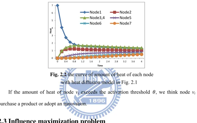
Fig 2.2 illustrates the curves of the variation of amount of heat of each node with heat diffusion model in Fig 2.1 (X-axis indicates time and Y-axis indicates amount of heat). We could see that only node 1 has heat at time 0. With time elapsing, the amounts of heat of other nodes are increasing and more close. Besides, assume node 2 is non-activated, but it can still spread information to node 5.

Fig. 2.2 the curve of amount of heat of each node

with heat diffusion model in Fig. 2.1

If the amount of heat of node vi exceeds the activation threshold , we think node vi

purchase a product or adopt an innovation.

2.3 Influence maximization problem

The problem of influence maximization [21] posed by Domingos and Richardson is stated below: if we can try to convince a subset of individuals to adopt a new product and the goal is to trigger a large cascade of further adoptions, which set of individuals should we target in order to achieve a maximized influence? In reality, a person’s decision to buy the product is often strongly influenced by his friends and acquaintances. That is to say, the influence maximization problem is how we select the most influential early adopters. Better early adopters cause the more people to adopt the product. Online social networks provide good opportunities to address this problem, since we can easily share information with our friends. Influence maximization problems under the LTM, ICM and HDM are all

0 1 2 3 4 5 6 7 0 0.4 0.8 1.2 1.6 2 2.4 2.8 3.2 3.6 4 Heat Time Node1 Node2 Node3,4 Node5 Node6 Node7

9  NP-problems, as already proved in [5, 6].

2.4 Community Detection Algorithm

A community is characterized as a subset of individuals who interact with each other more frequently than other individuals outside the community [22]. Community discovery is similar but not equivalent to the conventional graph partitioning problem. Both community discovery and conventional graph partitioning problem aim to cluster vertices into groups. A key challenge for the former, however, is that the algorithm has to decide what is the “the best“, or in other words, the “most natural“ partition of a network. In this thesis, we need the “most natural” partitioning without providing any information such as the number of partitions. Furthermore, if there is no good community structure, the network needs not be partitioned. That is why we use the community detection algorithm rather than conventional graph partitioning algorithm.

A quantitative measure, called modularity (Q), was proposed [7] to assess the quality of community structures, and community discovery was formulated as an optimization problem. Because Optimizing Q is an NP-problem, several heuristic methods have been proposed, as surveyed in [8]. Assume M is the number of edges and N is the number of nodes. The time complexity of most community detection algorithms are between O(NlogN) and O(N3). In this thesis, the efficiency of algorithms are most concerned, so we select KCUT [9] and SHRINK [10], which have low time complexity O(MlogN), as our community detection algorithms. Besides, the two algorithms are not only efficient but also have good modularity. We will briefly introduce the Kcut and SHRINK algorithms in the section 2.4.1 and 2.4.2.

2.4.1 Kcut Algorithm

Kcut algorithm [9] is spectral graph partitioning. There is a family of methods on spectral graph partitioning. These methods depend on the eigenvectors of the Laplacian

matrix of a graph. Depending on the way a graph is partitioned, spectral methods can be classified into two classes. The first class uses the leading eigenvector of a graph Laplacian to bi-partition the graph. The second class of approaches computes a k-way partitioning of graph using multiple eigenvectors. We briefly review some representative algorithms of these two classes below.

SM algorithm [11], the representative of first class, works as follows. SM computes , the second smallest generalized eigenvector of Laplacian matrix. Then a linear search is conducted on to find a partition of the graph to minimize a normalized cut criterion [11]. To find more than two clusters, the SM algorithm can be applied recursively

The representative of second class is NJW algorithm. NJW algorithm [12] finds a k-way partition of a network directly, where k is given by the user. NJW computes the k smallest generalized eigenvectors of Laplacian matrix and stack them in columns to form a matrix Y = [ , , ..., ]. Each row of Y is normalized to have unit length. NJW treats each row as a

point in , and then applies standard k-means algorithm to group these points into clusters. Kcut is a unique combination of recursive partitioning and direct k-way method. Kcut will achieve the efficiency of a recursive approach, while also having the same accuracy as a direct k-way method. It has been empirically observed that if there are multiple communities, using multiple eigenvectors to directly compute a k-way partition is better than recursive bi-partitioning method [12]. To optimize the performance measure of modularity Q, Kcut algorithm uses a greedy strategy to recursively partition a network. Unlike the most algorithms that always seek a bi-partition, it adopts a direct k-way partitioning. In summary, we compute the best k-way partition with k = 2,3,…, using the NJW algorithm, and select the k that gives the highest Q value. Then for each subnetwork, the algorithm is recursively applied.

Given a network G and a small integer l that is the maximum number of partitions to be considered for each subnetwork and Q is the value of modularity , Kcut executes the steps as

11  shown in Algorithm 1:

Algorithm 1: Kcut

Input : Graph of social network G; l : the maximum number of partitions to be considered

for each subnetwork

Output: Г : set of clusters

1. Initialize Г to be a single cluster with all vertices, and set Q=0. 2. For each cluster P in Г,

3. Let g be a subnetwork of G containing the vertices in P; 4. For each integer k from 2 to l

5. Apply NJW to find a k-way partitioning of g, denoted by Г ; 6. Compute new Q value of network as =Q(Г ∪ Г \ p ); 7. Find the k that gives the best Q value, i.e., k* = argmaxk ;

8. If ∗ > Q

9. accept the partition by replacing P with Г ∗, i.e., Г = Г ∪ Г ∗ \ P,

10. and set Q = ∗ ;

11. Advance to the next cluster in Г, if there is any;

Fig 2.3 is an example network for Kcut. Assume l is 3. Fig 2.4 is the eigenvectors of Laplacian matrix of Fig 2.3 and stack them in columns to form a matrix [ , , ]. Apply

NJW to find a k-way partitioning of Fig 2.3. We find k = 2 that gives the best Q value. Fig 2.5 is the partitioning of Fig. 2.3. Then no more partitioning could gain the modularity.

2.4.2 SHRINK Algorithm

SHRINK [10] is a parameter-free hierarchical network clustering algorithm by combining the advantages of density-based clustering and modularity optimization methods. It uses density-based method to quickly know which set of nodes may be the same cluster. Then it uses modularity optimization to decide whether results of clustering are good or not. It not only detects hierarchical communities, but also identifies hubs and outliers. Therefore, local connectivity structure of the network is used in SHRINK. We briefly review the details

Fig. 2.5 Two communities detected by Kcut

Fig. 2.4 Eigenvectors of Laplacian matrix of Fig 2.3 and

stack them in columns to form a matrix [ , , ]      Node 1  Node 2  ...               

13  of SHRINK as follows.

Given a weighted undirected network G = (V, E, w.). w(e) is the weight of edge e. We formalize some notions and properties of the hierarchical structure-connected clusters. Firstly, we define the structure similarity. The structural similarity effectively denotes the local connectivity density of any two adjacent nodes in a weighted network. For a node u ∈ V, we define w({ u, u }) = 1. The structure neighborhood of a node u is the set Г(u) containing u and its adjacent nodes : Г(u) = ∈ | , ∈ ∪ . The structural similarity between two adjacent nodes u and v is then

σ u,v = ∑ ∈Г ∩Г , ∙ ,

∑ ∈Г , ∙ ∑ ∈Г ,

. (2.6) Therefore, if node u and node v have more mutual and familiar friends, structure similarity of {u, v} will be higher. The above structural similarity is extended from a cosine similarity used in [13]. It can be replaced by other similarity definitions such as Jaccard similarity. However, [10] shows that the cosine similarity is better. We define the dense pair. σ u, v is the structure similarity of nodes u and v. If σ u, v is the largest similarity between nodes u, v and their adjacent neighbor nodes: σ u, v = max{ σ , y | (x = u, y ∈ Г ⋁ , y ∈ Г }, then {u, v} is called a dense pair in G.

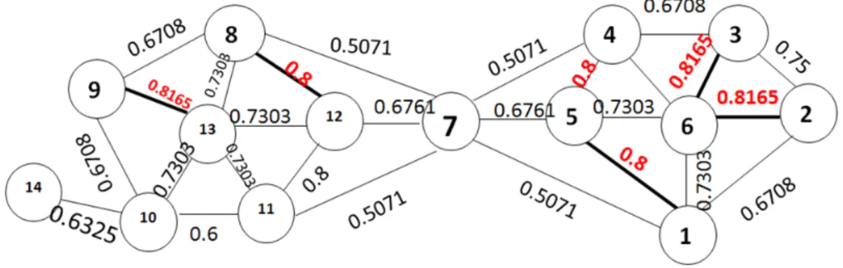
That is to say, a dense pair {u, v} is the largest similarity edge from all edges of u and v. As shown in Fig 2.6, {9,13} is a dense pair with structure similarity 0.8165 in the example network since {9, 13} is the largest similarity edges from all edge of node 9 and 13.

Fig.2.6 Illustration of the procedure and

result of the hierarchical network clustering algorithm SHRINK.

The main process can be divided into two phases that are repeated iteratively. Given a network with N nodes, first we initialize each node with a different community label. In this initial partition, the number of communities is the same as the number of nodes. Then, for each node u we combine the corresponding nodes in the dense pairs of u to form a super-node. This process is applied sequentially for all nodes. We record all different communities which represent a partition of the network. The second phase of the algorithm is to build a super-network. We evaluate the modularity gain of Qs for the shrinkage of the communities

found during the first phase. If the modularity gain is positive, the corresponding local (b)  1st iteration 2nd iteration Stop when △Qs < 0  (c)  (a) 

15 

community is replaced by a super-node. The above two phase are executed in turns until there is no community with positive modularity gain. For an example in Fig 2.7(a), at 1st iteration, we separately combine node set {9, 13}, {8, 11, 12}, {1, 4, 5} and {2, 3, 6} as four super nodes with structure similarity 0.8165, 0.8, 0.8, and 0.8165. Then since the modularity gains after shrinkage of communities are positive, the above four node sets are replaced by four super nodes. At 2nd iteration, node set {{8, 11, 12}, {9, 13}, 10} and {{1, 4, 5}, {2, 3, 6}} are separately combined as two super-nodes with 0.7303 and 0.7303. The modularity gains after shrinkage of communities in 2nd are positive, so we replace two node set {{8, 11, 12}, {9, 13}, 10} and {{1, 4, 5}, {2, 3, 6}} by their super-nodes. Since no more shrinkage of communities could gain the modularity gain of Qs, SHRINK stops. Then the hierarchy of

communities naturally occurs, as shown in Fig 2.7(b). Fig 2.7(c) represents final two-layers overlapping communities. Since node 7 connects two communities, it is a hub. In addition, node 14 is identified as an outlier which is loosely connected with the community {8, 9, 10, 11, 12, 13}.

SHRINK is not only efficient but also accurate. Besides, it can detect hubs which are very useful information in maximal influence problem. We could see that in the same graph in Fig 2.6 and Fig 2.3, Kcut only detect two communities, but SHRINK detect not only two communities but also a hub, node 7. Hub is very useful for influence maximization problem.

2.5 Seeds Selection Algorithm

We discuss previous works for seeds selection in this section. Influence maximization problem is an NP-problem. Hence, many works have been proposed to achieve approximate solutions. In social network, we often consider the person who has the most friends as the most influential person, since he can possibly influence most people. Therefore, the intuitive strategy, in general, is selecting seeds based on their degree, called degree centrality. Nevertheless, the members of large communities often have larger degree than other members

of smaller communities. Consequently, degree centrality easily selects seeds in the same large community. Influence spreads of each seed in the same community tend to be overlapped. As a result, degree centrality does not have good performance on influence spread. Distance centrality is another common used method for influence maximization problem. It selects seeds in the order of increasing average distance to other nodes. However, nodes in the larger communities usually have smaller average distance. As a result, most seeds may also be clustered. Simply stated, degree centrality and distance centrality result in the phenomenon of clustering of seeds, which deteriorates sharply in influence spread.

Pable A. Estevez et al. proposed set cover greedy algorithm [2] under independent cascading model (ICM). It kept selecting node with highest “uncover degrees”. Once a node is selected, all its neighbors as well as itself are labeled as “covered”. This procedure continues until k seeds are selected. This algorithm is computationally fast under simpler models, i.e., ICM. However, it has good influence spread only in high successful probability. The Climbing-up greedy algorithm [6] under ICM and LTM was proposed by David kempe et al.. They also provided the first provable 1 approximation guarantees for influence spread. The number e is Euler’s number. Recently, since social network websites are getting more popular, we have to pay more attention to efficiency of algorithms. In reality, at the beginning of the innovation diffusion process, several seeds in the network spread the information at the same time, not just one single seed. The information from his (her) social network may come from several seeds. At each iteration of climbing-up greedy algorithm, we select most “influential” node on the condition of considering all seeds selected before. This procedure continues until k seeds are selected. If a node could make more nodes to be activated, it seems to be more “influential”. For selecting the most influential node, we have to compute each node’s influence. Due to the heavy computing load of climbing-up greedy algorithm, it is not appropriate for large social networks. Besides, [5] proposed enhance greedy algorithm under heat diffusion model, i.e. the climbing-up greedy algorithm specially

17 

under heat diffusion model. Nevertheless, enhance greedy algorithm is also a climbing–up greedy algorithms. Consequently, we cannot solve influence maximization problem under heat diffusion model in acceptable time.

Yitong Wang et al [14] proposed a potential-based node selection. It selects some inactive

nodes that might not be optimal at starting phase but could trigger more nodes in later stage of diffusion. It can save half time of totally using Climbing-up greedy algorithm and cause more adoptions than that in [6]. However, in practice it is still not efficient enough. Therefore, the extremely efficient algorithm, degree discount heuristic, was presented by Wei Chen et al. [15]. It obtains the approximate solutions in large datasets for only a few seconds. Besides, its performance is close to [6]. However, both of [14, 15] are only under LTM or ICM, which are not very realistic diffusion models. In addition, degree discount heuristic is only for very low successful probability, i.e., people are extremely hard to be influenced in very low successful probability.

Chapter 3

Community Degree Heuristic (CDH)

In this chapter, we will describe our community degree heuristic (CDH) that quickly detect seeds under the heat diffusion model. In section 4.1, we present the overview of the system architecture and explain principles of CDH. In section 3.2 and 3.3, we will go into details about our CDH-Kcut and CDH-Shrink.

3.1 Overview of System Architecture

CDH is the unique combination of the community detection algorithm and modified degree centrality. Suppose we have data on a social network which has N individuals. The problem we need to solve is: given the quota number k, how to select the initial k “influential” individuals who will be delivered a free sample product, in order to maximize the number of cascade adoptions by which these individuals will influence their friends or individuals on their direct contact list.

In this thesis, we model social network marketing process by heat diffusion process. Initially, we select k individuals as seeds for heat diffusion, denoted by the set Sand the k seeds are given a certain amount of heat h0. At time zero of the heat diffusion process, we set

fi (0) = h0 , where i ∈ . As time elapses, the heat will diffuse through the whole social

network. If the amount of heat of individual i at time t is greater than or equal to an activation threshold , this individual i will be considered as having been successfully influenced on activated by others, and will adopt the product. We define the influence set of the set of k individuals S, denoted as (t), to be the expected number of individuals who will adopt the product at time t. Now the above problem could be interpreted as: finding the most influential k-size set S to maximize the size of set (t) at time t, where (t) ={ | , } .

19 

This problem is NP-hard, as already proven in [5]. We select the heat diffusion model to be our diffusion model since it can realistically simulate the real world.

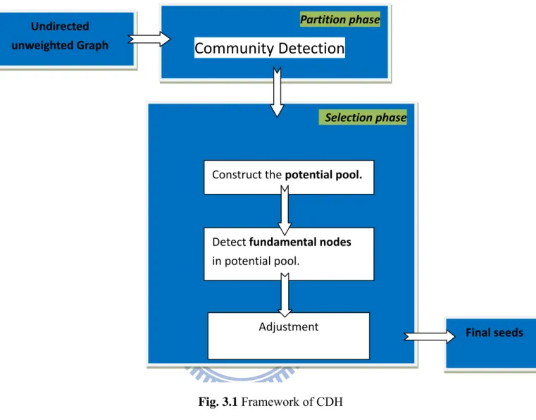
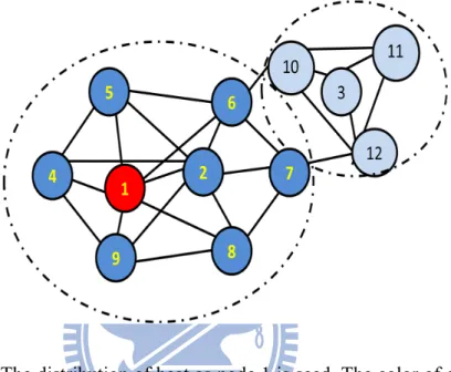
The proposed CDH is composed by two phases, partition phase and selection phase. Fig. 3.1 illustrates the framework of CDH. The first phase, partition phase, detects the communities of the network. Community is a subset of individuals who interact with each other more frequently than other individuals outside the community. In real life, one’s information often spread in his or her circle of friends. That is, most of someone’s influence clearly spread in his or her community. We find the same phenomenon in heat diffusion model. In Fig. 3.2, node 1 is a seed. The color of each node means its amount of heat. More dark blue means larger amount of heat. Nodes circled by dotted circle are in the same community. We

Fig. 3.1 Framework of CDH   Selection phase   

Community Detection 

can see that most gains of heat are in the community of node 1. In Fig 3.3, node1 and node 2 are seeds. Most gains of heat are also in the community of node 1. Nodes in the other community gains very little amount of heat. We can conclude that if we choose nodes in the same community as seeds, most gains of heat are in their own community. Other communities gain little amount of heat. Therefore, information of community is a very useful tool to avoid influence overlapping in heat diffusion model.

/

Fig. 3.2. The distribution of heat as node 1 is seed. The color of each

node means its amount of heat. More dark blue means larger amount of heat. Nodes circled by dotted line are in the same community.

Fig. 3.3. The distribution of heat as node 1 and node 2 are seeds. The

color of each node means its amount of heat. More dark blue means larger amount of heat. Nodes circled by dotted line are in the same community.

21 

The reason for using community detection algorithms rather than conventional graph partitioning algorithm is that we want to detect “the best”, or in other words, the “most natural“ partitioning of a network without providing any information such as the number of partitions. For example, if the network is natural to be partitioned to 3 communities, we should not force the network to be partitioned to 4 communities.

The second phase, selection phase, finds the most influential nodes based on the result

of partition phase and parameters of heat diffusion model, such as flow duration, thermal conductivity and activation threshold. In Fig. 3.4, community 1 is a larger community than community 2. It shows that select nodes from community 1 as seeds instead of nodes from community 2 could trigger more individual to be activated. The degrees of each node in social network also fit with power-law distribution [17, 18], i.e., a very large number of nodes have very small numbers of neighbors. Hence, most large-degree nodes are in large communities. Due to the above reasons, we only consider nodes in the large communities as seed candidates.

Fig. 3.4 Comparison with three seeds in different community size.

Community 1 is a larger community than community 2. Select the same number of seeds from community 1 could trigger more individuals to be activated than from community 2.

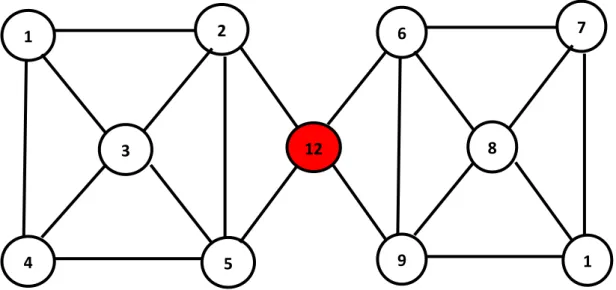
The candidates are put in the potential pool. Therefore, we intend to select seeds from potential pool. Next, we detect the “fundamental node” from the potential pool. Fundamental nodes have more potential to be seeds since it has larger degree than that of other nodes in the same community, or it is located on the important position in the network. The important position means connecting many communities. Fig. 3.4 and 3.5 show two kinds of fundamental node. In Fig.3.4, node 3 is the fundamental node. It has the largest degree among all nodes. In Fig. 3.5 node 12 is the fundamental node. It has better position which can easily influence two node sets {1,2 , 3, 4, 5 } and {6, 7, 8, 9, 11}

1

2

4

5

3

Fig 3.4. An example of Fundamental node. Node 3 is the

fundamental node. It is has the largest degree among all nodes.  

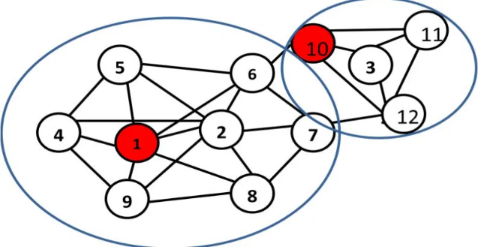
Fig. 3.5. An example of fundamental node. Node 12 is the fundamental node. It has better

position which can easily influence two node sets {1, 2, 3, 4, 5} and {6, 7, 8, 9, 11}.

1  2  4  5  3  6  7  9  1 8  12

23 

How to detect the fundamental nodes is one of differences between CDH-Kcut and CDH-Shrink algorithms. Although these nodes have good chance to become the final seeds, they are not the best seeds in different situations (parameters) of heat diffusion model. For example, seeds which perform well in short flow duration may not be good in long flow duration. Therefore, adjusting the fundamental nodes to become more ideal seeds is essential.

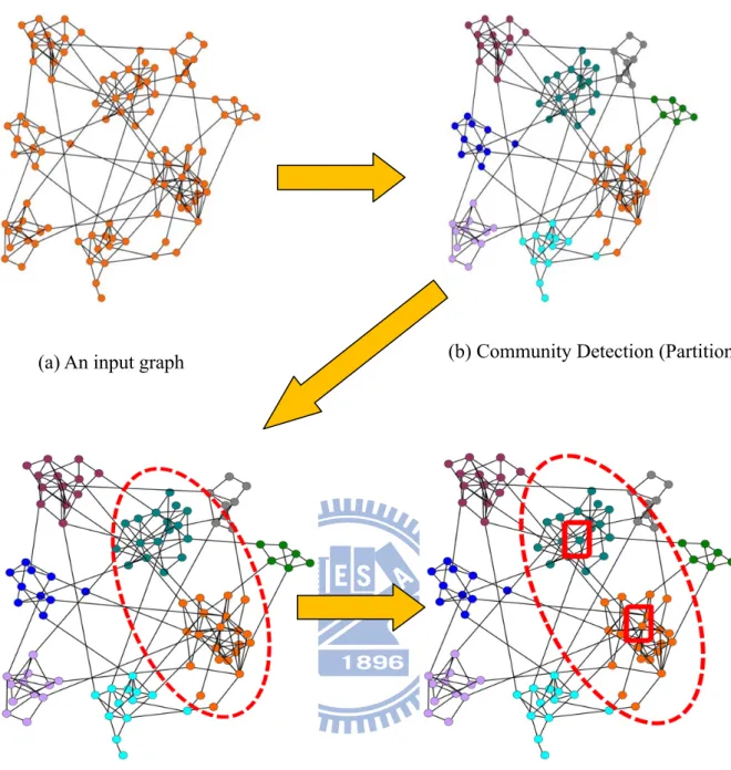
(a) An input graph (b) Community Detection (Partition Phase)

(c) Construct potential pool (selection phase) (d) Find fundamental nodes in potential pool (assume two fundamental nodes)

Fig. 3.6(a) is an example of input graph. Fig. 3.6(b) is the result of community detection of Fig. 3.6(a). Different color means different community. After partition phase, the first step of selection phase is constructing the potential pool. Two communities circled by red dotted circle are potential pool since the two communities are the two largest communities among all communities in Fig. 3.6(c). Assume two fundamental nodes are to be selected. Fig. 3.6(d) shows two fundamental nodes in the potential pool since they have large degree. After the step of constructing potential pool and finding fundamental nodes, we effectively narrow down the scope of seed candidates. CDH-Kcut and CDH-Shrink are two algorithms using different community detection algorithms and different strategies of potential pool, fundamental nodes and adjustment. We explain details of two algorithms in next two sections.

25 

3.2 CDH-Kcut

CDH-Kcut is composed of partition phase and selection phase. The purpose of partition phase is to detect communities. The selection phase finds the influential nodes in communities. The strategies used by the CDH-Kcut are presented below:

(Partition phase):

We partition the network into communities by Kcut algorithm [9]. Every node will belong to only one community, and overlapping community is not allowed in Kcut. We assume the graph G is partitioned to the l communities. In most cases, l is larger than k, so in this paper we don’t discuss the case l < k.

(Selection phase)

After detecting communities, we have l communities. If we want to find k seeds, firstly we construct the potential pool, PP(G). We define potential pool as :

, , … , , (3.1)

where is the set of top-p degree nodes in i-th largest community SCi, i = 1,2,..,k.

Therefore, PP(G) keeps the top-p degree nodes in each community of top-k largest communities. In most cases, p = 10% of community size is enough for selecting good seeds. Therefore, we significantly narrow down the range of possible seeds. Then, we select the fundamental nodes from the potential pool. Since Kcut cannot identify importance of location of nodes in each , degree has been considered as the only attribute that distinguishes good fundamental nodes from poor fundamental nodes. Thus, we select the largest degree node in each as the fundamental nodes. S ={s1,s2,….,sk} is the set of seed candidates si..

Fundamental nodes are seed candidates. Fig. 3.7 is an example of finding fundamental nodes. Node 1 and node 7 are the largest degree nodes in respective community. Finally, we adjust the fundamental nodes to be the final seeds. Our basic idea of adjustment is a heuristics that tries to use an add-node a_node to replace a delete-node d_node. If the influence spread after node replacing is larger than before replacing, we do the replacement,

Algorithm 1: CDH-Kcut

Input : Graph of social network G ; number of total seeds k, Parameters p Output: k seeds

1. Execute the Kcut(G) ;

2. Select top-k biggest communities from the communities in Kcut(G) ; 3. foreach selected community SCi do

4. Add top-p degree nodes into set ; 5. end

6. foreach do

7. select the most degree node Si from ;

8. End

9. IM = Is(t);//Is(t): influence spread of current seed set, IM : record max influence spread

10. foreach community SCi do

11. if size(SCi) > avg(∑ size ) then

12. Add SCi in LC ; //LC : the set of large communities

13. end 14. end

15. Sort LC based on community size ; 16. ci = 0 ; // ci : community index 17. di = 0; // di : index of d_node 18. foreach Ci in LC

19. ai = 2 ; //ai : index of a_node 20. while ture do

21. Select the ai-th large degree node from as a_node; 22. Select the seed candidates sk-di from S as d_node;

23. if Is(t) < IM then

24. Cancel the replacement in line 21 and line 22. 25. break ; 26. end 27. IT= Is(t); 28. ai = ai +1; 29. di = di +1; 30. End 31. ci = ci +1; 32. end 33. Output individuals in S

27  else we cancel the replacement.

As in Fig 3.3, seeds selected from large community could trigger more adoptions than that selected from small community. As a result, we incline to select add-node in large communities and delete-node in the small communities since we want to know whether selecting nodes from large communities can gain more influence spread or not. If the size of a community is larger than AvgSC = avg(∑ size ), then this community is deemed as large community. Notice that delete-nodes must be fundamental nodes. Due to the adjustment, we can avoid influence spread from being spoiled for the effect of different value of parameters, such as flow duration, activation threshold and thermal conductivity. We discuss the effect of flow duration, activation threshold and thermal conductivity individually. Comparing the difference caused by long time and short time, information will diffuse farther in long flow duration. That is, in long flow duration the seeds would influence more individuals than that in short low duration. Therefore, we should not select too many seeds in one community in long flow duration. In contrast, it is appropriate selecting more seeds in one community in short flow duration.

It is more difficult to make individuals adopt products in high activation threshold. Individuals need more heat to be activated in higher activation threshold, so we tend to select more seeds in one community with high activation threshold.

Fig. 3.7 An example of finding fundamental nodes in

High thermal conductivity makes information diffuse more quickly. Compare with low

thermal conductivity, information of high thermal conductivity makes information diffuse longer distance. Hence, we do not select many seeds in one community. We conclude that differences caused by different parameters are the level of seeds clustering. In the simulation of short flow duration, high threshold and low thermal conductivity it is better to select more seeds in one community, i.e., higher level of seed clustering. On the other hand, long flow duration, low threshold and high thermal conductivity social network, not many seeds in one community is needed, i.e., lower level of seed clustering. Therefore, the adjustment in CDH-Kcut is to test and verify whether large communities should need more seeds. Lines between 9 and 29 in algorithm 1 show the steps in seeds adjustment.

29 

3.3 CDH-Shrink

Our proposed CDH-Shrink is also composed of two phase, partition phase and selection

phase. Besides, Shrink algorithm [10] could detect hub, i.e., a node connecting different communities. It provides us more information about the community structure property. The communities detected by Shrink are more precise than by Kcut. Due to above reasons, we can select more productive fundamental nodes than in CDH-Kcut. We describe it as follows:

(Partition phase):

We get information of community structure and hubs by Shrink algorithm.

(Selection phase):

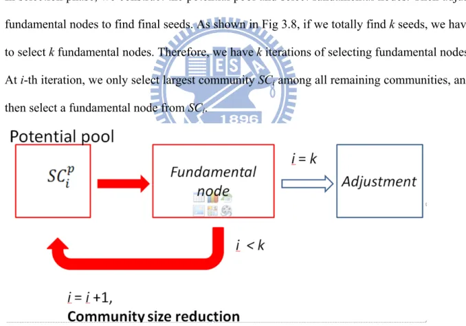
In selection phase, we construct the potential pool and select fundamental nodes. Then adjust fundamental nodes to find final seeds. As shown in Fig 3.8, if we totally find k seeds, we have to select k fundamental nodes. Therefore, we have k iterations of selecting fundamental nodes. At i-th iteration, we only select largest community SCi among all remaining communities, and

then select a fundamental node from SCi.

Fig 3.8. Flowchart of selection phase. Assume select k seeds. We have k

iterations of selecting fundamental node. Before selecting the fundamental node of ,the size of each community covered by the fundamental node of has to reduce the degree of fundamental node of . PP(G) ={ , ,…, }. : top-p degree nodes in i-th largest community. p: 10% of community size. i= 1~k

We first select top-p degree nodes from SCi, denoted as . p = 10% of SCi’s size is enough

to select good fundamental nodes. Before selecting the fundamental node of , the size of each community covered by the fundamental node of has to reduce the degree of fundamental node of . As shown in Fig. 3.9, assume that node 7 is the fundamental node in C1. The size of C2 will be reduced to 3. Community size reduction is for reducing the

influence overlapping. Fundamental nodes should “cover” communities as much as possible while having much influence on their communities. In Fig.3.10, node u belongs to community C1, C2 and C3. That is, u covers C1, C2 and C3.

C

C1

C

Fig. 3.10 An example of “cover”. C1, C2 and C3 are

communities. Node u belongs to C1, C2 and C3. That is, u

covers C1, C2 and C3.

C

C

Fig 3.9 Illustration of community size reduction.

We select node 7 as the fundamental node in C1. The

size of C2 will be reduced to 3.

8  1 9  1 1 1 1 1 7 3  2 4 6  5 1 

31 

To select good fundamental nodes, we define “position_score” as:

position_score(u) = |{Ci | u ∈ Ci , u ∈ ∈ set of communities | , (3.2)

to evaluate the importance of node’s position in network. If the node u is a nonhub, the position_score(u) is 1. Otherwise, the position_score(u) is the number of communities which u belongs to. We also define “hub_purity” as:

hub_purity(h) = | | ∈ , ∈ _{_} ∉ |, (3.3) where FC is the set of communities which contain fundamental nodes and h is a hub. In Fig. 3.11¸ C1 and C2 are communities containing fundamental node u. C1, C2 and C3 are

communities containing node z. C2 and C4 are communities containing node v. Therefore,

purity(z) = 1/3 and purity(v) = 1/2.

We choose the “MAX priority” nodes from as fundamental nodes, i = 1,2..,k. Selecting fundamental nodes in CDH-Shrink is different from that in CDH-Kcut. Function

compare_priority shows how to compare priority of nodes. If both nodes are hub, we

compare their position_score other than their degree. We compare hub with hubsize since we want to cover more communities. That is, we want to choose the hub which has important positions in the network. Besides, if the node is a hub, its purity must exceed the threshold of purity. We do not want to select low-purity fundamental nodes to reduce information overlapping. The hub with low purity easily covers too many covered communities, and this

z 

v 

u 

C

C

C

C

Fig 3.11 An example of how to computing purity. C1, C2,

C3 and C4 are communities. Node u is the fundamental

hub, consequently, has the lowest priority while comparing purity. When comparing nonhub with hub or nonhub, we compare their influence on their neighbors, i.e., degree, due to no information about importance of location of non_hubs. After comparing top-p degree nodes in SCi , we can find the fundamental node. The fundamental node may have a very good

position which connecting SCi with many other communities or have much influence on their

neighbors or have both. S ={s1,s2,….,sk} is the set of seed candidates si.Fundamental nodes

are seed candidates

Finally, we adjust fundamental nodes to be final seeds. Adjustment in CDH-Shrink is also a heuristics. Try to choose an add-node to replace a delete-node. Then test whether the influence spread after replacing is larger than that before replacing. left and seedLoad play important roles in adjustment. left and seedLoad help us to determine add-nodes and delete-nodes . We define “left” and “ seedLoad“ as:

left(Ci) = the number of non-activated nodes in community Ci, (3.4)

seedLoad(Ci) = _{| | ∈ , ∈ |} , (3.5)

Left(Ci) might be thought of as “the need of adding more seeds in Ci “. As left(Ci) is

increasing, the need of selecting more seeds in Ci is increasing. Implied in the seedLoad(Ci) is

whether too many seeds in Ci. When seedLoad(Ci) is small, that, perhaps, means too many

seeds in Ci..

In each iteration, we select the add-node a_node , where

a_node = u | max{∑ left | ∈ , ∈ G(V), t = position_score(u) } .

In the meanwhile, we select a delete-community d_comm, which has the smallest seedLoad among SC, SC ={SC1,SC2,…SCk}. Then select delete-node d_node which has minimun

size(A(d_node)) among all seeds in d_comm. A(u) is a set of active nodes adjacent to node u. We test if we should substitute add-node a_node for delete-node d_node. If the influence spread after substitution is more than that before, we make a substitution. To quickly find a

33 

productive a_node, we do not consider very low degree node. We could assume selecting low degree nodes as seeds is not productive. Lines between 15 and 34 in CDH-Shrink show the details of adjustment. The adjustment has r iterations to test the substitution. In most cases, r = 2k~3k is efficient to get satisfactory influence spread.

            Algorithm 2: CDH-Shrink 

Input : Graph of social network G ; number of total seeds k, Parameters p,

purity_threhold , adjustment time r

Output: k seeds

1. Execute the Shrink(G); 2. while |SC| < k do

3. Add the biggest community SCi into SC;

4. // select the fundamental node 5. foreach top-p degree nodes in SCi do

6. //ni : the i-th largest degree node in SCi

7. maxnode = compare(ni, maxnode);

8. end

9. Si = maxnode;

10. foreach community Ci which has max do 11. Size(Ci) = Size(Ci) – degree(max);

12. end 13. end

14. //adjustment

15. IM= Is(t); // Is(t) : influence spread of current seed set, IM : record max influence spread 16. for 1 to r do

17. select a_node = u | max{ ∑ left | ∈ , u ∈ G(V), 18. t = position_score(u)} ;

19. select _ argmin _∈

20. select _ argmin _{∈ , ∈} | | ∈ , ⊆ |

Function compare_priority (node a, node b)

1. if a is hub and hub_purity(a) < purity_threshold  2. return b 

3. if a is hub and b is hub then 

4. return max( position_score(a), position_score ( b )); 5. else if a is nonhub then

6. return max(degree(a), degree( b)); 7. end

21. delete d_node in S and add a_node into S ; 22. if Is(t) < IM then

23. Cancel the replacement between line18 to 22. 24. end

25. IM = Is(t) ; 26. end

27. Output individuals in S

3.4 Time Complexity of Approximation Algorithms

We now consider the time complexity of CDH-Shrink, CDH-Kcut and enhance greedy algorithm [5]. Suppose that a social network is composed of N individuals and M edges. The time complexity of heat diffusion process is O(RM )[5], which means the number of iterations R multiplied by the number of edges M in a social network. In most cases, R = 30 is enough for approximating the heat diffusion process. We select k seeds. The complexity of each algorithm is as follows:

For CDH-Kcut, l is the number of communities. Each top-k community selects top-p degree nodes in potential pool. The partition phase in CDH-Kcut is O(MlogN). Assume average number of nodes in a community is . Constructing the potential pool is O(kp ). Finding fundamental nodes in potential pool is O(kp). Finding large communities is O(k). Assume we have b large communities. Sorting large communities is O(blogb). Adjustment in CDH-Kcut is O(kRM). Therefore, the time complexity is O(MlogN + kp + kp + k + blogb+ kRM).

For CDH-Shrink, assume the number of adjustment iterations is r, and the average community number of a node is d. The partition phase is O(MlongN). The time complexity of community size reduction is O(d), so finding fundamental nodes in potential pool is O(k(l + p +d)). In the adjustment, selecting add_node is O(Nd+N), selecting delete_community is O(k), and selecting delete_node is O(k). Therefore, the time complexity of adjustment in

35 

CDH-Shrink is r(Nd + N + k + k + RM). The total time complexity is O(MlogN + k(l + p +d) + r(Nd + N + k + k + RM)).

The time complexity of greedy algorithm in enhance greedy algorithm is O(kNCM) since selecting a seed is O(NRM) and we have to select k seeds. In most cases, r = 2k ~3k is enough for adjustment. We could see that in terms of time complexity, the ranking is CDH-Shrink CDH-Kcut greedy algorithm in [5]. 

Chapter 4

Experiments

To measure the performance of our proposed algorithms, we conduct experiments on a co-authorship network [26], the zachary’s karate network from Newman [25], the network of facebook, and two synthetic networks. The goal of the experiments is to show that our algorithms are very efficient and with satisfying influence spread.

We run the following set of algorithms under heat diffusion model.  EGA: the original enhanced greedy algorithm [5].

 CDH-Kcut: the community and degree heuristic. Community detection algorithm used is Kcut. .

 CDH-Shrink: the community and degree heuristic. Community detection algorithm used is SHRINK.

 DH: As a baseline, a simple degree heuristic that selects the k nodes with the largest degrees.

The performance metrics of the algorithms compared and the parameter setting are listed below.

1. Influence spread (number of activated nodes) 2. Efficiency (running time)

3. Effect of different values of parameters - t : flow duration

- θ : activation threshold - α :thermal conductivity

37 

4.1 Synthetic Networks

For synthetic datasets, we use the Lancichinetti-Fortunato-Radicchi (LFR) benchmark graphs [19, 20] to evaluate the performance of our algorithms. Some important parameters of the synthetic networks are:

 N: number of nodes  M: number of edges  maxd: maximum degree

 mp: mixing parameter, each nodes shares a fraction mp of its edges with nodes in other communities.

As shown in Table 4.1, we generate five different undirected graphs : (1) 1000Smp : the graph with 1000 nodes and small mixing parameter; (2) 1000Lmp : the graph with 1000 nodes and large mixing parameter; (3) 1000Lmaxd : the graph with 1000 nodes and large maximum degree; (4) 1000LM : the graph with 1000 nodes and large number of degree; (5) 5000Smp : the graph with 5000 nodes and small mixing parameter. Generally, the higher the mixing parameter of a network is, the more difficult to reveal the community structure.

Dataset N M maxd mp 1000Smp 1000 9097 100 0.1 1000Lmp 1000 9097 100 0.5 1000Lmaxd 1000 9097 200 0.1 1000LM 1000 22484 100 0.1 5000Smp 5000 47094 100 0.1 d

Table 4.1: The parameters of the omputer-generated datasets

Table 4.2 provides the result of different algorithms with different activation threshold, flow duration and thermal conductivity in 1000Smp. The influence spreads of CDH-Shrink and CDH-Kcut from θ = 0.2 to θ = 1.4 are almost the same or slightly different. Thus, we only report θ = 0.2, θ=1.5 and θ = 2.0. We can see that CDH-Shrink and CDH-Kcut have same influence spread in most cases and even are better than EGA with θ = 2.0. Fig. 4.1 shows 5 seed selected by CDH-Kcut with t=0.1, θ=0.1, α=0.1 in 1000Smp. Fig. 4.2 shows 5 seed selected by CDH-Kcut with t=0.1, θ=0.1, α=0.1 in 1000Smp. We could see that higher activation threshold leads to the phenomenon of seed clustering.

          network EGA CDH-Shrink CDH-Kcut DH

t=0.1, θ=0.1, α=0.1 1000Smp 341  339  339  215  t=0.1, θ=0.2, α=0.1 1000Smp 336  332  332  215  t=0.1, θ=1.5, α=0.1 1000Smp 223  201  197  95  t=0.1, θ=2.0, α=0.1 1000Smp 133  141  166  95  t=0.2, θ=0.1, α=0.1 1000Smp 386  367  345  336  t=0.3, θ=0.1, α=0.1 1000Smp 503  482  499  472  t=0.4, θ=0.1, α=0.1 1000Smp 635  594  649  567  t=0.1, θ=0.1, α=0.2 1000Smp 386  367  345  336  t=0.1, θ=0.1, α=0.3 1000Smp 503  482  499  472  t=0.1, θ=0.1, α=0.4 1000Smp 635  594  649  567 

Table 4.2: Influence spread with 4 different algorithms in 1000Smp. t

39                _{Fig 4.2 5 Seeds (red nodes) selected by CDH-Kcut with t=0.1, θ=2.0,}

α=0.1 in 1000Smp.

Fig 4.1 5 Seeds (red nodes) selected by CDH-Kcut with t=0.1, θ=0.1,

Table 4.3 shows the influence spread with 4 different algorithms with different activation threshold, flow duration and thermal conductivity in 1000Lmp. CDH-Kcut performs worse than CDH-Shrink in 1000Lmp since SHRINK could detect more accurate community structure than Kcut. Hence, if it is hard to get correct community structure of the graph, CDH-Shrink will probably perform better than CDH-Kcut. Besides, accuracy of detected community structure reflects the performance of influence spread of CDH-Shrink and CDH-Kcut. Therefore, with increasing of mixing parameter, the performance of influence spread of CDH-Shrink and CDH-Kcut have deteriorated.

Table 4.4 indicates the influence spread with 4 different algorithms with different activation threshold, flow duration and thermal conductivity in 1000Lmaxd. Nodes in 1000Lmaxd could have larger degree. That is, some nodes’ degree will be extremely larger   network EGA CDH-Shrink CDH-Kcut DH

t=0.1, θ=0.1, α=0.1 1000Lmp 251  223  213  206  t=0.1, θ=0.2, α=0.1 1000Lmp 225  182  175  187  t=0.1, θ=1.5, α=0.1 1000Lmp 176  157  149  105  t=0.1, θ=1.6, α=0.1 1000Lmp 137  121  93  56  t=0.2, θ=0.1, α=0.1 1000Lmp 562  491  467  484  t=0.3, θ=0.1, α=0.1 1000Lmp 790  734  712  722  t=0.4, θ=0.1, α=0.1 1000Lmp 892  841  813  829  t=0.1, θ=0.1, α=0.2 1000Lmp 562  491  467  484  t=0.1, θ=0.1, α=0.3 1000Lmp 790  734  712  722  t=0.1, θ=0.1, α=0.4 1000Lmp 892  841  813  829 

Table 4.3: Influence spread with 4 different algorithms in 1000Lmaxd.

41 

than the others. Consequently, performance of influence spread of DH will be improved, especially in high activation threshold.

Table 4.5 shows the influence spread with 4 different algorithms with different activation threshold, flow duration and thermal conductivity in 1000LM. In 1000LM, each node has more neighbors, so information will spread quickly. Hence, we could see that influence spread in 1000LM is higher than that in 1000Smp, 1000Lmp and 1000Lmaxd. In most cases, the influence spreads of CDH-Shrink and CDH-Kcut are still better than DH.

Table 4.6 indicates that influence spread with 4 different algorithms with different activation threshold, flow duration and thermal conductivity in 5000Smp. 5000Smp has 5000 nodes. In most cases, the influence spread of CDH-Shrink and CDH-Kcut are still better than DH.

  network EGA CDH-Shrink CDH-Kcut DH

t=0.1, θ=0.1, α=0.1 1000Lmaxd 332 315 298 202 t=0.1, θ=0.2, α=0.1 1000Lmaxd 290 278 259 196 t=0.1, θ=1.5, α=0.1 1000Lmaxd 170 151 143 146 t=0.1, θ=1.6, α=0.1 1000Lmaxd 138 110 113 136 t=0.2, θ=0.1, α=0.1 1000Lmaxd 494 493 473 299 t=0.3, θ=0.1, α=0.1 1000Lmaxd 565 569 561 404 t=0.4, θ=0.1, α=0.1 1000Lmaxd 627 610 599 482 t=0.1, θ=0.1, α=0.2 1000Lmaxd 494 493 473 299 t=0.1, θ=0.1, α=0.3 1000Lmaxd 565 569 561 404 t=0.1, θ=0.1, α=0.4 1000Lmaxd 627 610 599 482

Table 4.4: Influence spread with 4 different algorithms in 1000Lmaxd.