Why fishing magnifies fluctuations in fish abundance

ARTICLES

Why fishing magnifies fluctuations in fish

abundance

Christian N. K. Anderson

, Chih-hao Hsieh

, Stuart A. Sandin

, Roger Hewitt

, Anne Hollowed

,

John Beddington

, Robert M. May

& George Sugihara

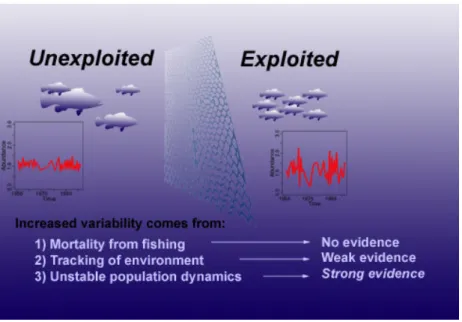
It is now clear that fished populations can fluctuate more than unharvested stocks. However, it is not clear why. Here we distinguish among three major competing mechanisms for this phenomenon, by using the 50-year California Cooperative Oceanic Fisheries Investigations (CalCOFI) larval fish record. First, variable fishing pressure directly increases variability in exploited populations. Second, commercial fishing can decrease the average body size and age of a stock, causing the truncated population to track environmental fluctuations directly. Third, age-truncated or juvenescent populations have increasingly unstable population dynamics because of changing demographic parameters such as intrinsic growth rates. We find no evidence for the first hypothesis, limited evidence for the second and strong evidence for the third. Therefore, in California Current fisheries, increased temporal variability in the population does not arise from variable exploitation, nor does it reflect direct environmental tracking. More fundamentally, it arises from increased instability in dynamics. This finding has implications for resource management as an empirical example of how selective harvesting can alter the basic dynamics of exploited populations, and lead to unstable booms and busts that can precede systematic declines in stock levels.

Ecologists have long suspected that harvesting a species has the unin-tended consequence of destabilizing the abundance of that species1,2_. This would be undesirable, because boom-and-bust cycles can increase the likelihood of local extinctions3_{and can harm the} eco-nomic market for the species. However, this connection has been remarkably difficult to prove. A historic example is the collapse of the California sardine fishery in the late 1940s, which some argued was caused primarily by fishing4,5_{, but which others attributed to} cooling sea surface temperatures or to shifting wind patterns6–8_. Because landings records contain no information about unexploited species, there is no control group to disentangle environmental effects from fishing effects. Partly to address this conundrum, CalCOFI was initiated to collect data both on fished and unfished species living in the same environment. CalCOFI overcame the reli-ance on landings data by sampling the ichthyoplankton assemblage, a well-known proxy for current adult (spawning) biomass9–11_{. Fifty} years into the study, Hsieh et al.9_{used the CalCOFI ichthyoplankton} database12_{to separate the effects of fishing from other variables, and} demonstrated that fishing significantly increases temporal variability of populations in the southern sector of the California Current eco-system (Fig. 1). Increased variability is thought to be related to the truncated age/size structure3,4,9,13–17_{of commercially fished species, a} phenomenon caused by selective removals of larger, older individuals that previously provided stability to the population.

Here we examine three competing hypotheses for the link between fishing and stock variability1,2,9,16,18_{. First, fishing itself can vary year} to year and this can translate directly into increased population variability19_{. Second, fished populations that become dominated by} relatively small-bodied and young individuals are less able to smooth out environmental fluctuations, and are thus more likely than unfished stocks to track directly those fluctuations4,9,13_{. Finally,}

fished populations that become dominated by small-bodied and young individuals are more prone to exhibit unstable dynamics due to changing demographic parameters20,21_{. These are not mutually}

1

Scripps Institution of Oceanography, University of California, San Diego, La Jolla, California 92093, USA.2Center for Ecological Research, Kyoto University, Hirano, 2-509-3, Otsu, 520-2113, Japan.3_{Institute of Oceanography, National Taiwan University, No. 1, Section 4, Roosevelt Road, Taipei, 10617, Taiwan.}4_{Institute of Marine Environmental Chemistry and}

Ecology, National Taiwan Ocean University, 2, Pei-Ning Road, Keelung, 20224, Taiwan.5_{Southwest Fisheries Science Center, National Marine Fisheries Service, 8604 La Jolla Shores}

Drive, La Jolla, California 92037, USA.6_{Alaska Fisheries Science Center, National Marine Fisheries Service, 7600 Sand Point Way NE, Seattle, Washington 98115, USA.}7_{Division of}

Biology, Faculty of Natural Sciences, Imperial College London, RSM Building, South Kensington Campus, London SW7 2AZ, UK.8_{Department of Zoology, University of Oxford, South}

Parks Road, Oxford OX1 3PS, UK.

Age at maturity

95% Confidence interval of abundance:mean

1 2 3 4 5 6

5:1

1:1

1:5

1:10

Figure 1|In addition to an increased coefficient of variation9_{, exploited}

species (red dots) exhibit larger booms and busts than unexploited species (blue triangles) of a similar age. The 95th and the 5th percentiles of abundance are shown for each species, with exponential fits (dashed lines) for the exploited and unexploited species. Note that for all species, the busts (lower range) are more pronounced than the booms (P , 0.0001). Populations less than one-tenth mean size probably fell below detection levels and were conservatively fixed at one-tenth mean size; thus, the effect may be more pronounced than depicted here.

Vol 452|17 April 2008|doi:10.1038/nature06851

835

Nature Publishing Group

exclusive hypotheses; all three could act together to increase variabi-lity. Here we analyse the relative importance of each hypothesis as a cause of the increase in population variability of fished stocks observed in the southern California Current ecosystem.

Hypothesis 1 (variable fishing)

According to hypothesis 1, a fish stock is expected to vary more if exploited heavily some years and lightly in others. Jonze´n et al.22 discovered a positive correlation between the variance in fishing mortality and the variance in the standing stock biomass of Baltic cod populations. We use their method on the CalCOFI database, to test this hypothesis for the seven exploited species whose fishing mortality is available from National Marine Fisheries Service stock assessment reports (Supplementary Table 1) and find no evidence that variability in fishing mortality is associated with variability in either larval density (Fig. 2) or estimated spawning biomass (Supplementary Fig. 2). Therefore, although it is reasonable to expect the variability of these populations to be somewhat influenced by year-to-year differences in fishing effort, hypothesis 1 alone does not explain the observed increase in variability of these data. Hypotheses 2 and 3 (age-truncation effects)

The other two hypotheses are closely related. Because fishing typically targets the larger individuals of a species, the average size—and thus age—of target populations is often found to decrease14–16,18,23_{. Age} truncation leading to increased population variability has been docu-mented in several populations9_{, and is here referred to as the ‘age} truncation effect’ (ATE)13_{. Such juvenescence can affect population} variance in two separable ways.

Hypothesis 2 suggests that when new recruits compose most of the stock, the juvenescent population is more likely to track variable environmental processes directly4,5_{. Although younger and smaller} fish are more susceptible to changes in the environment, older and larger fish tend to integrate over environmental fluctuations and survive hard times better through ‘bet-hedging’ strategies18,24–27 including fat storage, the ability to migrate and avoid poor areas, having flexibility in spawning times and locations, and production of high-quality offspring that survive in a broader suite of environ-mental conditions18_{. Bet-hedging strategies are well documented in}

association with long-tailed age distributions18,24–27_{. Loss of hedging} capacity through age truncation should produce a time-series signal that more closely exhibits the linear (statistically noisy) characteris-tics found in physical oceanographic data for that region21_.

By contrast, under hypothesis 3, the increased variability of exploited fish stocks comes from changes in demographic parameters that amplify nonlinear behaviour20,21_{. There are many ways that the} ATE can change demographic parameters, for example by increasing intrinsic population growth rates or by increasing nonlinear coupling of demographic parameters to environmental noise20,28_{. The} result-ing population dynamics will produce a more variable time series with more nonlinear behaviour than seen in unexploited fish stocks. Separating environment and demography

Because hypothesis 2 implies increased tracking of linear environ-mental variation, whereas hypothesis 3 describes an enhanced non-linear response, we can distinguish these subtle alternatives by comparing the nonlinearity in the time series of exploited species relative to unexploited species. Here, nonlinearity is quantified using S-maps29_{, a model validation criterion that uses out-of-sample} pre-dictions from equivalent linear versus nonlinear models to identify the dynamics behind time-series observations. The model either weights all data equally (h 5 0) to make linear forecasts, or gives more weight to data points with similar recent histories (h . 0), a hallmark of nonlinear behaviour29,30_{. The nonlinearity of a time series is} deter-mined by how much the correlation (r) between forecasts and observations increases as models are tuned towards nonlinear solu-tions; that is, how much forecast skill increases (Dr) when h . 0 (Dr 5 rh . 0– rh 5 0; see Methods).

When CalCOFI ichthyoplankton time series are modelled using linear autoregression (S-maps with h 5 0), fished species are slightly more predictable than unfished species (r 5 0.514 and 0.504, respec-tively; Fisher’s test P 5 0.64; Supplementary Fig. 3). However, this possible evidence for hypothesis 2 is marginal (Supplementary Table 2). Indeed, nonlinear models describe the CalCOFI ichthyoplank-ton time series better (h 5 0.3 for both), and more importantly, fished species exhibit significantly more nonlinearity than the unfished group (Fig. 3a; unfished Dr 5 0.037, P 5 0.25; fished Dr 5 0.083, P , 0.01; Fisher’s test, P , 0.003). If the increase in variance is due to vulnerable, young fish simply tracking the linear environment more closely, then the nonlinearity (Dr) of fished species should decrease. This prediction is contradicted by the data.

r = 0.113 P = 0.412 r = 0.004 P = 0.983 r = –0.039 P = 0.879 r = 0.038 P = 0.920 Three-year window 2 1 0 1 2 2 2 1 0 1 2 2 Five-year window

Seven-year window Ten-year window

CalCOFI data 0.08 0.06 0.04 0.02 0.00 ∆ r 0.08 0.06 0.04 0.02 0.00 ∆ r Unexploited Exploited a Model results Unexploited Hypothesis 3 b

Rather, fishing pressure has enhanced the nonlinear behaviour of the fished populations. Therefore, the data suggest that altered dynamics resulting from a truncated age structure overwhelm the propensity of young fish to track the environment passively and that dynamic instability is the agent behind the observed increase in variance. Increased nonlinearity has explained higher variance in other contexts29,31_.

Identifying sources of nonlinearity

We illustrate the distinction between hypotheses 2 and 3 with a population growth model having the familiar Ricker-form29,32

Nt115Ntexp[r(1 2 Nt)] 1 ce (1) where N is population size (in units of number or biomass), r is the intrinsic population growth rate, e is environmental variability with unit standard deviation, and c is environmental susceptibility (see Methods, Supplementary Fig. 4 and Supplementary Discussion). Hypothesis 2 corresponds to an increase in environmental suscep-tibility c; hypothesis 3 corresponds to alteration of a demographic parameter: for this example we increase r. Forecast skill does not improve with nonlinear tuning (h . 0) as environmental noise (ce) is increased, but declines with h, as would be expected if the time series were dominated by linear statistical effects (Fig. 3b, dashed line; see Methods). We find this result is maintained whether e is ‘white’ noise, autocorrelated ‘red’ noise, 1/f ‘pink’ noise or the actual values of the Pacific Decadal Oscillation33–35_{. However, under hypothesis 3} (Fig. 3b, solid red line), exploited model populations present an enhanced nonlinear signature as r is increased.

At first glance, it seems counterintuitive that age truncation would increase intrinsic population growth rates (because fishing removes the largest individuals that produce the most and best qua-lity eggs18,24–27_{); yet this trend is observed empirically in the California} Current ecosystem. Because individual body size decreased and total biomass remained statistically constant (26 of 29 stocks9_{), the} num-ber of young fish has increased. A larger population of shorter-lived fish requires a higher intrinsic rate of growth (r); the population must produce more surviving offspring per capita per year to compensate for the shortened life span. The ultimate mechanism behind this ATE-induced increase could be competitive release and/or decreased cannibalism or possibly evolution23,36,37_{, leading to increased somatic} growth or increased per-capita fecundity. Although other factors are probably operating, the evidence from CalCOFI points to increased growth rates as a dominant factor supporting the increase in non-linearity observed in Fig. 3a.

Although it is well known that increasing growth rates in simple discrete growth models can lead to unstable dynamics38_{, values of r} required to evoke such behaviour in single species models are often unrealistically high. However, models with multiple species39_, mul-tiple stable states28_{or models having demographic parameters that} vary in complex ways with the environment20,21_{produce nonlinear} behaviour even at modest growth rates. More generally, process noise (error from incompletely specified models) can induce instability in otherwise stable models when the error multiplies in specific ways; that is, when an essential detail is added that has a nonlinear effect. Using the commonly studied29 _{form of process noise Z}

t115 G(Zt1eprocess) where equation (1) is an example of G, Fig. 4 shows that generic process noise evokes nonlinear behaviour at lower growth rates. This toy representation portrays nonlinear or biologi-cally amplified process errors.

Thus, increasing either process noise or growth rates can amplify nonlinearity. And fishing may affect both. For example, incorporat-ing variable fishincorporat-ing Ftinto equation (1) so that variability in F is an expression of process noise,

Nt115Ntexp[ri(1 2 Nt/Kt2Ft)] (2) leads to amplified nonlinearity (Fig. 5). (However, the lack of a relation in Fig. 2 eliminates this as a cause for increased variability in these data.) Similarly, modelling process errors more explicitly by adding variability directly to the demographic parameters r or K in equation (2) will provoke a nonlinear signature, regardless of the particular form of the noise (see Methods and Supplementary Fig. 5). It is reasonable to speculate that the baseline nonlinearity seen in the unexploited state is an expression of nonlinear process errors related to variable demographic parameters, such as those tied to ecosystem shifts and climate events for example8,9,20_{. So, although} neither variability in fishing nor in the environment correlates with variability in abundance, these two sources of process error may be implicated in complex ways with the instability that accompanies fishing. Notwithstanding their potential destabilizing effects, by themselves these processes have little direct effect on the overall stock variability we observed in CalCOFI (Fig. 2, Supplementary Fig. 2, and Supplementary Tables 2 and 3).

Life-history traits and nonlinearity

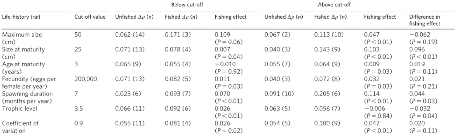
Are there characteristics that make some fish stocks more susceptible to the nonlinear effects of fishing than others? To answer this ques-tion we compared the nonlinearity of exploited and unexploited stocks for various life-history traits (Table 1 and Supplementary Table 4). Table 1 identifies a qualitative tendency for the following characteristics to be associated with vulnerability to fishing: larger size at sexual maturity ($25 cm), greater age at sexual maturity ($3 years), longer spawning duration (.7 months), higher fecun-dity ($200,000 eggs per female per year), lower trophic level and

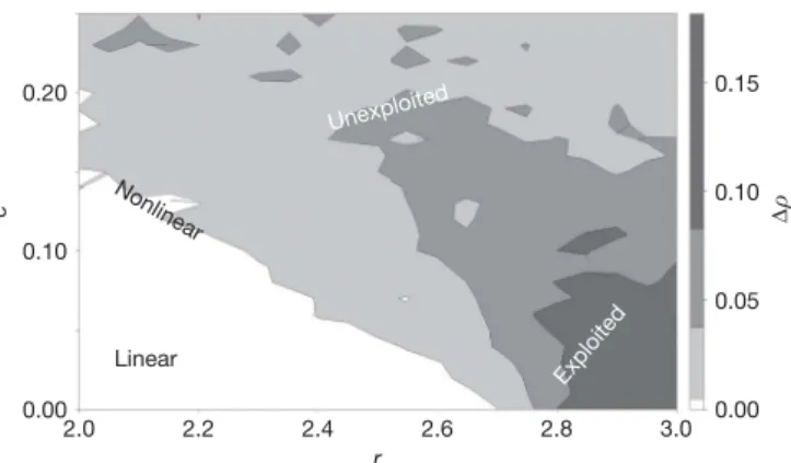
0.20 0.15 0.10 0.05 0.00 c 0.10 0.00 2.0 2.2 2.4 2.6 r 2.8 3.0 Nonlinear Linear Unexploited Exploited ∆ r

Figure 4|Nonlinear behaviour can emerge at modest growth rates (r) with process noise (eprocess).Models that are underspecified (missing important

components) are said to contain process noise. In this example, we evaluate the nonlinearity of Zt115G(Zt1eprocess), where G is equation (1) and

eprocessis normally distributed with mean 0 and standard deviation c. Process

noise can amplify a nonlinear signature in the simple model for values of r that would be linear alone.

∆ r 0.00 0.05 0.10 0.15 0.20 0.06 0.04 0.02 0.00

Coefficient of variation (parameter) Variable r Variable K

Variable F

Figure 5|Variable fishing F (dotted line), growth r (solid line), or carrying capacity K (dashed line), can induce nonlinearity.

NATURE|Vol 452|17 April 2008 ARTICLES

837

Nature Publishing Group

more variability in abundance (coefficient of variation $ 0.9). Thus, acknowledging the uncertainty arising from the small number of species involved in some groups, one may speculate that to a first approximation, large-maturing lower-trophic-level species that are also fecund, may be most susceptible to further destabilization by fishing, and regardless of life history the evidence suggests that increasing growth rates are driving this effect.

Management implications

In summary, fishing for big individuals without consideration of the impact on the age distribution can lead to unstable nonlinear popu-lation dynamics, and this enhanced nonlinearity helps to explain much of the volatility seen in fish stocks today (Fig. 1). Our study shows that when unconstrained, an observed demographic con-sequence of the ATE, that is, the effective increase of r, makes dra-matic population change more likely—and paradoxically, in this case, can make those changes slightly more predictable in the short run. Thus target species are in double jeopardy from both fishing removals and the ATE, as stocks with higher mortality also suffer increasing fluctuations. Reduced size and age distributions have been documented in many common fisheries species, for example in Pacific salmon40_{, Pacific rockfish}41_{, and North Sea ground fish}42,43_, suggesting the potential relevance of the ATE for many commercially important species. In terms of stock recovery, it can be premature therefore to resume fishing activities solely on the basis of recovery of biomass but before restoration of historical age distributions, even though short-term industry pressures may make this difficult to realize (for example, Atlantic swordfish44_).

It is encouraging, however, that some managers are adopting precautionary harvest policies that protect against stock depletion and the ATE45,46_{. For example, in Alaska, where fishing is managed} through a complex system of harvest controls, there has been rela-tively minor impact on the mean age of the population47,48_.

Hypotheses 2 and 3 were tested with S-maps on composite CalCOFI ichthyo-plankton time series, using methods described in detail elsewhere21,50_{. Briefly,}

larval time series were composited end-to-end, and nonlinearity of fished versus unfished species was assessed by computing Dr with an embedding dimension E 5 3 (Supplementary Materials).

Hypotheses 2 and 3 are illustrated with a simple model (equation (1)) whose behaviour is generic to a large class of fisheries models (Supplementary Discussion). First, a baseline is established by fitting parameters to the observed variance (Supplementary Fig. 6) and nonlinearity of unexploited CalCOFI popu-lations (Fig. 3b, blue line). Next, to model hypothesis 2, environmental suscep-tibility (c) is increased to simulate direct environmental tracking with the ATE (Fig. 3b, dashed line). Alternative types of environmental noise were simulated for hypothesis 2 (red, 1/f, white, low-pass filtered and the actual Pacific Decadal Oscillation values33–35_{), and did not affect the qualitative outcome. Finally,}

hypo-thesis 3 is here simulated by increasing species-specific growth rates (r) (Fig. 3b, solid red line). Various forms of process noise were also simulated. All standard statistical analyses were performed with R software version 2.3.0.

Received 12 November 2007; accepted 22 February 2008.

1. Beddington, J. R. & May, R. M. Harvesting natural populations in a randomly fluctuating environment. Science197, 463–465 (1977).

2. May, R. M., Beddington, J. R., Horwood, J. W. & Shepherd, J. G. Exploiting natural populations in an uncertain world. Math. Biosci.42, 219–252 (1978).

3. Lande, R., Engen, S. & Saether, B. Stochastic Population Dynamics in Ecology and Conservation (Oxford Univ. Press, New York, 2003).

4. Murphy, G. I. Vital statistics of the Pacific sardine (Sardinops caerulea) and the population consequences. Ecology48, 731–736 (1967).

5. Murphy, G. I. Population biology of the Pacific sardine (Sardine caerulea). Proc. Calif. Acad. Sci. 4th ser.34, 1–84 (1966).

6. Marr, J. C. in Proc. World Sci. Meeting Biol. Sardines Related Species (eds Rosa, H. & Murphy, G.) 667–791 (FAO, Rome, 1960).

7. Clark, F. N. & Marr, J. C. Population dynamics of the Pacific sardine. CalCOFI Prog. Rep.4, 11–48 (1955).

8. Rykaczewski, R. R. & Checkley, D. M. Jr. Influence of ocean winds on the pelagic ecosystem in upwelling regions. Proc. Natl Acad. Sci. USA105, 1965–1970 (2008). 9. Hsieh, C. H. et al. Fishing elevates variability in the abundance of exploited species.

Nature443, 859–862 (2006). Table 1|Vulnerability of species with different life histories to destabilization by fishing

Below cut-off Above cut-off

Life-history trait Cut-off value Unfished Dr (n) Fished Dr (n) Fishing effect Unfished Dr (n) Fished Dr (n) Fishing effect Difference in fishing effect Maximum size (cm) 50 0.062 (14) 0.171 (3) 0.109 (P 5 0.06) 0.067 (2) 0.113 (10) 0.047 (P , 0.01) 20.062 (P 5 0.19) Size at maturity (cm) 25 0.071 (13) 0.078 (4) 0.007 (P 5 0.04) 0.040 (3) 0.143 (9) 0.103 (P , 0.01) 0.096 (P , 0.01) Age at maturity (years) 3 0.065 (9) 0.055 (4) 20.010 (P 5 0.92) 0.055 (7) 0.064 (9) 0.009 (P 5 0.03) 0.019 (P 5 0.11) Fecundity (eggs per

female per year)

200,000 0.071 (13) 0.082 (5) 0.011 (P 5 0.03) 0.040 (3) 0.072 (8) 0.032 (P 5 0.03) 0.021 (P 5 0.21) Spawning duration

(months per year)

7 0.023 (6) 0.093 (7) 0.070 (P , 0.01) 0.091 (10) 0.205 (6) 0.114 (P , 0.01) 0.044 (P 5 0.03) Trophic level 3.5 0.066 (11) 0.092 (6) 0.026 (P , 0.01) 0.063 (5) 0.056 (7) 20.006 (P 5 0.84) 20.032 (P 5 0.04) Coefficient of variation 0.9 0.055 (11) 0.081 (4) 0.026 (P 5 0.02) 0.054 (5) 0.100 (9) 0.047 (P , 0.01) 0.020 (P 5 0.11)

Species are separated into groups on the basis of having life-history traits above or below a cut-off value, and the nonlinearity (Dr) of exploited and unexploited species within these groups is compared. Significance is calculated by jack-knifing the data set, S-mapping and then comparingDr distributions of the fished and unfished data (one-tailed P values). Fishing significantly increased the nonlinearity of 12 of the 14 groups investigated. To evaluate which life-history traits are most impacted by fishing, the differences inDr values were compared (two-tailed P values in the right-hand column). Qualitatively, susceptibility to fishing is greater in late-maturing, fecund, low-trophic-level species with year-round spawning and high variability.

18. Berkeley, S. A., Hixon, M. A., Larson, R. J. & Love, M. S. Fisheries sustainability via protection of age structure and spatial distribution of fish populations. Fisheries 29, 23–32 (2004).

19. Jonzen, N., Ripa, J. & Lundberg, P. A theory of stochastic harvesting in stochastic environments. Am. Nat.159, 427–437 (2002).

20. Dixon, P. A., Milicich, M. J. & Sugihara, G. Episodic fluctuations in larval supply. Science283, 1528–1530 (1999).

21. Hsieh, C. H., Glaser, S. M., Lucas, A. J. & Sugihara, G. Distinguishing random environmental fluctuations from ecological catastrophes for the North Pacific Ocean. Nature435, 336–340 (2005).

22. Jonzen, N., Lundberg, P., Cardinale, M. & Arrhenius, F. Variable fishing mortality and the possible commercial extinction of the eastern Baltic cod. Mar. Ecol. Prog. Ser.210, 291–296 (2001).

23. Jorgensen, C. et al. Managing evolving fish stocks. Science318, 1247–1248 (2007).

24. Lambert, T. C. Duration and intensity of spawning in herring Clupea harengus as related to the age structure of the population. Mar. Ecol. Prog. Ser.39, 209–220 (1987).

25. Marteinsdottir, G. & Steinarsson, A. Maternal influence on the size and viability of Iceland cod (Gadus morhua) eggs and larvae. J. Fish Biol.52, 1241–1258 (1998). 26. Hutchings, J. A. & Myers, R. A. Effect of age on the seasonality of maturation and

spawning of Atlantic cod, Gadus morhua, in the northwest Atlantic. Can. J. Fish. Aquat. Sci.50, 2468–2474 (1993).

27. Bobko, S. J. & Berkeley, S. A. Maturity, ovarian cycle, fecundity, and age-specific parturition of black rockfish (Sebastes melanops). Fish. Bull.102, 418–429 (2004). 28. Steele, J. H. & Henderson, E. W. Modeling long-term fluctuations in fish stocks.

Science224, 985–987 (1984).

29. Sugihara, G. Nonlinear forecasting for the classification of natural time series. Phil. Trans. R. Soc. Lond. A348, 477–495 (1994).

30. Sugihara, G., Grenfell, B. & May, R. M. Distinguishing error from chaos in ecological time series. Phil. Trans. R. Soc. Lond. B330, 235–250 (1990). 31. Sugihara, G. et al. Residual delay maps unveil global patterns of atmospheric

nonlinearity and produce improved local forecasts. Proc. Natl Acad. Sci. USA96, 14210–14215 (1999).

32. Hilborn, R. & Walters, C. J. Quantitative Fisheries Stock Assessment: Choice, Dynamics and Uncertainty (Chapman and Hall, New York, 1992).

33. Halley, J. M. Ecology, evolution and 1/f-noise. Trends Ecol. Evol.11, 33–37 (1996). 34. Steele, J. H. A comparison of terrestrial and marine ecological systems. Nature

313, 355–358 (1985).

35. Vasseur, D. A. & Yodzis, P. The color of environmental noise. Ecology85, 1146–1152 (2004).

36. Conover, D. O. & Munch, S. B. Sustaining fisheries yields over evolutionary time scales. Science297, 94–96 (2002).

37. Kuparinen, A. & Merila, J. Detecting and managing fisheries-induced evolution. Trends Ecol. Evol.22, 652–659 (2007).

38. May, R. M. Biological populations with nonoverlapping generations: stable points, stable cycles, and chaos. Science186, 645–647 (1974).

39. Hastings, A. & Powell, T. Chaos in a three-species food chain. Ecology72, 869–903 (1991).

40. Ricker, W. E. Changes in the average size and average age of Pacific salmon. Can. J. Fish. Aquat. Sci.38, 1636–1656 (1981).

41. Harvey, C. J., Tolimieri, N. & Levin, P. S. Changes in body size, abundance, and energy allocation in rockfish assemblages of the northeast Pacific. Ecol. Appl.16, 1502–1515 (2006).

42. Armstrong, M., Dann, J. & Sullivan, K. Programme 1: North East Cod. Fisheries Science Partnership 2006/07 Final Report (Cefas, Lowestoft, 2006). 43. Poulsen, R. T., Cooper, A. B., Holm, P. & MacKenzie, B. R. An abundance estimate

of ling (Molva molva) and cod (Gadus morhua) in the Skagerrak and the northeastern North Sea, 1872. Fish. Res.87, 196–207 (2007).

44. ICCAT. Standing Committee on Research and Statistics (ICCAT-SCRS) Stock Status Report – Swordfish – North Atlantic 2006 (FAO, Rome, 2006). 45. Murawski, S. A., Rago, P. J. & Trippel, E. A. Impacts of demographic variation in

spawning characteristics on reference points for fishery management. ICES J. Mar. Sci.58, 1002–1014 (2001).

46. Stefansson, G. & Rosenberg, A. A. Combining control measures for more effective management of fisheries under uncertainty: quotas, effort limitation and protected areas. Phil. Trans. R. Soc. B360, 133–146 (2005).

47. Spencer, P. D., Hanselman, D. & Dorn, M. in Biology, Assessment, and Management of North Pacific Rockfishes. Univ. Alaska Sea Grant Program Report No. AK-SG-07–01 (eds Heifetz, J. et al.) 513–533 (Univ. Alaska Fairbanks, Fairbanks, Alaska, 2007).

48. Anonymous. Alaska Groundfish Fisheries Final Programmatic Supplemental Environmental Impact Statement (US Department of Commerce, National Oceanic and Atmospheric Administration, National Marine Fisheries Service, Alaska Region, Juneau, Alaska, 2004).

49. Sibert, J., Hampton, J., Kleiber, P. & Maunder, M. Biomass, size, and trophic status of top predators in the Pacific Ocean. Science314, 1773–1776 (2006). 50. Hsieh, C. H., Anderson, C. & Sugihara, G. Extending nonlinear analysis to short

ecological time series. Am. Nat.171, 71–80 (2008).

Supplementary Information is linked to the online version of the paper at www.nature.com/nature.

Acknowledgements We acknowledge support from National Oceanic and Atmospheric Administration Fisheries and the Environment, the McQuown Chair Endowment in Natural Science, the Deutsche Bank – Jameson Complexity Studies Fund, the Sugihara Family Trust, National Science Council-Long-term Observation Research of the East China Sea, the Center for Marine Bioscience and

Biotechnology, and a grant for Biodiversity Research of the 21st Century Center of Excellence at Kyoto University. M. Maunder, P. Hull, V. Dakos, S. Carpenter, J. Bascompte, M. Scheffer, C. Folke, E. H. van Nes, B. Brock, J. Murray, N. Yamamura and H.-H. Lee provided comments.

Author Contributions G.S., C.N.K.A, C.-h.H., R.M.M. and J.B. helped to frame the original research to investigate hypothesis 3. C.-h.H. and G.S. performed the initial S-map analysis on the CalCOFI data that verified hypothesis 3. C.N.K.A., with assistance from C.-h.H. and G.S., did the model analyses, statistical tests and the documentation of life-history results. All co-authors assisted with the evolution of the research plan and the refinement and final exposition of ideas.

Author Information Reprints and permissions information is available at www.nature.com/reprints. Correspondence and requests for materials should be addressed to G.S. ([email protected]).

NATURE|Vol 452|17 April 2008 ARTICLES

839

Nature Publishing Group

Supplementary Figures

Figure S1 | A schematic figure representing the main findings of this study.

SUPPLEMENTARY INFORMATION

Figure S2 | This figure reproduces Fig. 1, but with spawner biomass (SB) estimated

from fishery-dependent data (Table S1). The coefficient of variation in fishing mortality,

CV(F), does not correlate with variability in estimates of spawner biomass, CV(SB),

using a 3-, 5-, 7-, and 10-year moving window (r

=0.001, 0.030, 0.020, 0.029; P=0.8,

0.257, 0.454, 0.474 respectively). This analysis excludes pacific chub mackerel where

policy changes in the allowable catch in response to changes in spawning biomass

_,

introduced an artificial positive relationship. Even including these points, the relationship

is marginally significant only at the 5- and 7-year scale (r

_{=0.078, 0.123; P=0.041,}

0.034). Because there are several ways that fishery-dependent estimates of SB could

introduce an artificial relationship between SB and fishing mortality

, we view these null

results as conservative.

doi: 10.1038/nature06851

SUPPLEMENTARY INFORMATION

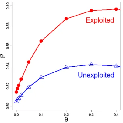
Figure S3 | The difference in predictability (ρ) at the y-intercept (where θ=0.0) shows

that a linear model makes slightly more accurate forecasts for exploited populations

(ρ

=0.516) than for unexploited population (ρ

=0.504

). However, the difference in

linear forecast skill is not significant (P=0.64, Fisher’s test), which lends only weak

support to hypothesis 2. Furthermore, this slight difference in predictability is dwarfed by

the gains in predictability evident when using a nonlinear model (θ=0.3). Here, the

difference between exploited and unexploited populations is much more apparent

(P=0.003, Fisher’s test), as would be expected under hypothesis 3. Note the y-axis of

this figure is the absolute forecast skill (ρ) of each model and not the difference from the

linear baseline (Δρ) as presented in Figures 3 and S2.

doi: 10.1038/nature06851

SUPPLEMENTARY INFORMATION

Figure S4 | Model results and observations for unexploited (blue, column 1) and

exploited populations (red, columns 2 & 3). (a) Hypothetical age structure of an

unexploited population. (b) Hypothetical age structure of an exploited population

showing age truncation. (c) Unexploited species would show a moderate growth rate r

and environmental susceptibility c in eqn 1. (d) The younger population may track the

environment more strongly and therefore deviate further from the growth function

(hypothesis 2 modelled by increasing c), or (e) the young population may change

demographic parameters (hypothesis 3 modelled by increasing r). Example time series

of species under (f) unexploited conditions or (g-h) two models of exploitation. Either

mechanism results in a population that fluctuates more dramatically through time.

S-maps of species modelled under three regimes: (i) unexploited, showing moderate

nonlinearity (a positive Δρ at θ>0, with a larger Δρ indicating more nonlinearity (Δρ =ρ

– ρ

); (j) exploited under hypothesis 2, showing less or no nonlinearity; (k) and

exploited under hypothesis 3, showing more nonlinearity. (l-m) Analysis of CalCOFI

ichthyoplankton data show that fished species show more nonlinearity than unfished

species.

doi: 10.1038/nature06851

SUPPLEMENTARY INFORMATION

Figure S5 | Allowing demographic parameters r or K to vary though time (where N

=

N

e

, see methods) causes the time series to appear more nonlinear, regardless

of the correlation structure of the variance. The larger the CV, the more nonlinear the

time series signature (standard deviations for each line are solid = 0, shortdash = 0.05,

dotted = 0.1, dash-dot = 0.2, longdash = 0.3). Similar results were obtained when fishing

mortality (F

) was given mean 0.3 and allowed to vary in N

= N

e

while r

and

K

were held fixed (see Methods).

Figure S6 | The coefficient of variation for a 40-point time series governed by (1) was

approximated by 96,100 time series with values of r in the range [0, 5] and c in the

range [0.00, 0.30]. The tangent to the CV surface at 0.8667 (the observed CV of

unexploited CalCOFI species) was approximated for the area delimited by the dashed

box. The parameter c was dropped from the tangent fit, because r alone was able to

explain more than 90% of the variation in CV in this region.

doi: 10.1038/nature06851

SUPPLEMENTARY INFORMATION

Supplementary Tables

Table S1. Data sources for the spawning biomasses and fishing mortality from stock assessment

reports for seven exploited species.

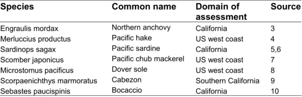
Species Common

name

Domain

of

assessment

Source

Engraulis mordax Northern anchovy California 3

Merluccius productus Pacific hake US west coast 4

Sardinops sagax Pacific sardine California 5,6

Scomber japonicus Pacific chub mackerel US west coast 7

Microstomus pacificus Dover sole US west coast 8

Scorpaenichthys marmoratus Cabezon Southern California 9

Sebastes paucispinis Bocaccio California 10

Table S2. The percent of variation (r

) in larval abundance explained by major environmental

indices for CCE species. No environmental variable explained more than 1.5%, and no

correlations were significant when Bonferroni corrected (* = P<0.05). (See also Hsieh et al.

_for

analyses on each individual species).

Physical time

series

Exploited species

Unexploited species

Abundance

(n=520)

ΔAbundance

(n=507)

Abundance

(n=640)

ΔAbundance

(n=624)

La Jolla SST 0.0086* 0.0000 0.0022 0.0008 ΔSST 0.0134* 0.0085* 0.0039 0.0011 La Jolla Salinity 0.0028 0.0000 0.0002 0.0005 ΔSalinity 0.0022 0.0013 0.0035 0.0052 Annual PDO 0.0002 0.0009 0.0000 0.0010 ΔPDO 0.0002 0.0002 0.0021 0.0002 Annual NPI 0.0005 0.0137* 0.0015 0.0087* ΔNPI 0.0038 0.0042 0.0026 0.0011 Annual SOI 0.0000 0.0003 0.0002 0.0007 ΔSOI 0.0007 0.0021 0.0013 0.0001

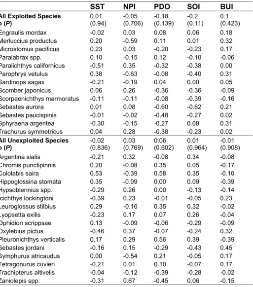
Table S3. The correlation coefficient (ρ) between the CV(ΔLarval density) and

CV(ΔEnvironmental Index) over a 5-year moving window. No significant correlations were

obtained for any single species (n=33 overlapping windows; critical values of |ρ| : 0.70 [P=0.05],

0.83 [P=0.01], and 0.92 [P=0.001]). No significant results were obtained with window sizes of 3,

7, or 10 years either.

SST NPI PDO SOI BUI

All Exploited Species

ρ (P) 0.01 (0.94) -0.05 (0.706) -0.18 (0.139) -0.2 (0.11) 0.1 (0.423) Engraulis mordax -0.02 0.03 0.08 0.06 0.18 Merluccius productus 0.20 -0.59 0.11 0.01 0.32 Microstomus pacificus 0.23 0.03 -0.20 -0.23 0.17 Paralabrax spp. 0.10 -0.15 0.12 -0.10 -0.06 Paralichthys californicus -0.51 0.35 -0.32 -0.38 0.00 Parophrys vetulus 0.38 -0.63 -0.08 -0.40 0.31 Sardinops sagax -0.21 -0.19 0.04 0.00 0.05 Scomber japonicus 0.06 0.26 -0.36 -0.36 -0.09 Scorpaenichthys marmoratus -0.11 -0.11 -0.08 -0.39 -0.16 Sebastes aurora 0.01 0.08 -0.60 -0.62 0.21 Sebastes paucispinis -0.01 -0.02 -0.48 -0.27 0.02 Sphyraena argentea -0.30 -0.15 -0.27 0.08 0.31 Trachurus symmetricus 0.04 0.28 -0.38 -0.23 0.02

All Unexploited Species

ρ (P) -0.02 (0.836) 0.03 (0.769) 0.06 (0.602) 0.01 (0.964) -0.01 (0.908) Argentina sialis -0.21 0.32 -0.08 0.34 -0.08 Chromis punctipinnis 0.20 -0.08 0.35 0.05 -0.17 Cololabis saira 0.53 -0.39 0.58 0.35 -0.10 Hippoglossina stomata 0.35 -0.09 0.00 0.09 -0.39 Hypsoblennius spp. -0.29 0.26 0.00 -0.13 -0.14 Icichthys lockingtoni -0.39 0.23 -0.01 -0.05 0.23 Leuroglossus stilbius 0.29 -0.16 0.35 0.32 -0.02 Lyopsetta exilis -0.23 0.17 0.07 0.26 -0.04 Ophidion scrippsae 0.13 -0.09 -0.06 -0.29 -0.09 Oxylebius pictus -0.46 0.37 -0.07 -0.24 0.32 Pleuronichthys verticalis 0.17 0.29 0.56 0.39 -0.39 Sebastes jordani -0.16 0.15 -0.29 -0.43 0.45 Symphurus atricaudus 0.00 -0.54 0.21 -0.05 0.17 Tetragonurus cuvieri -0.21 0.01 0.10 -0.07 0.17 Trachipterus altivelis -0.04 -0.12 -0.39 -0.28 -0.02 Zaniolepis spp. -0.31 0.67 -0.45 0.06 -0.15

doi: 10.1038/nature06851

SUPPLEMENTARY INFORMATION

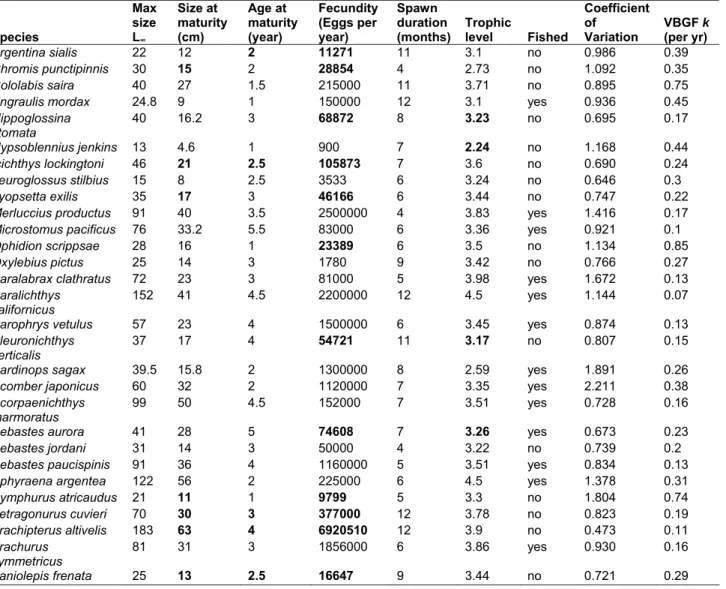
Table S4. Life history data for the CalCOFI fishes

. Missing data (bold) are imputed based on

their correlation structure

, using Expectation-Maximization algorithm assuming multivariate

normal distribution

_{. Many of these life history traits are related (as discussed in Hsieh et. al.}

2006). The growth rate from von Bertalanffy’s growth function (VBGF) is derived from prior

data using the relationship

L(t) = L

(1 - e

)

Æ

k = - [ln ( 1 - ( L(t) / L

)) / t] = - [( ln ( 1 - ( SSM / MaxSz )) / ASM]

(months) Trophic level Fished

Coefficient of

Variation VBGF k (per yr)

Argentina sialis 22 12 2 11271 11 3.1 no 0.986 0.39

Chromis punctipinnis 30 15 2 28854 4 2.73 no 1.092 0.35

Cololabis saira 40 27 1.5 215000 11 3.71 no 0.895 0.75

Engraulis mordax 24.8 9 1 150000 12 3.1 yes 0.936 0.45

Hippoglossina stomata 40 16.2 3 68872 8 3.23 no 0.695 0.17 Hypsoblennius jenkins 13 4.6 1 900 7 2.24 no 1.168 0.44 Icichthys lockingtoni 46 21 2.5 105873 7 3.6 no 0.690 0.24 Leuroglossus stilbius 15 8 2.5 3533 6 3.24 no 0.646 0.3 Lyopsetta exilis 35 17 3 46166 6 3.44 no 0.747 0.22

Merluccius productus 91 40 3.5 2500000 4 3.83 yes 1.416 0.17

Microstomus pacificus 76 33.2 5.5 83000 6 3.36 yes 0.921 0.1

Ophidion scrippsae 28 16 1 23389 6 3.5 no 1.134 0.85

Oxylebius pictus 25 14 3 1780 9 3.42 no 0.766 0.27

Paralabrax clathratus 72 23 3 81000 5 3.98 yes 1.672 0.13

Paralichthys californicus

152 41 4.5 2200000 12 4.5 yes 1.144 0.07

Parophrys vetulus 57 23 4 1500000 6 3.45 yes 0.874 0.13

Pleuronichthys

verticalis 37 17 4 54721 11 3.17 no 0.807 0.15 Sardinops sagax 39.5 15.8 2 1300000 8 2.59 yes 1.891 0.26

Scomber japonicus 60 32 2 1120000 7 3.35 yes 2.211 0.38

Scorpaenichthys

marmoratus 99 50 4.5 152000 7 3.51 yes 0.728 0.16 Sebastes aurora 41 28 5 74608 7 3.26 yes 0.673 0.23

Sebastes jordani 31 14 3 50000 4 3.22 no 0.739 0.2

Sebastes paucispinis 91 36 4 1160000 5 3.51 yes 0.834 0.13

Sphyraena argentea 122 56 2 225000 6 4.5 yes 1.378 0.31

Symphurus atricaudus 21 11 1 9799 5 3.3 no 1.804 0.74 Tetragonurus cuvieri 70 30 3 377000 12 3.78 no 0.823 0.19 Trachipterus altivelis 183 63 4 6920510 12 3.9 no 0.473 0.11 Trachurus symmetricus 81 31 3 1856000 6 3.86 yes 0.930 0.16 Zaniolepis frenata 25 13 2.5 16647 9 3.44 no 0.721 0.29

Supplementary Discussion

Comment on Generality of Results to Fisheries Models: Results in Fig. S4 (that show an

increase in population variability and nonlinearity with increased growth rates) are generic to

compensatory discrete-time fisheries population models where the growth curve steepens about

N

= N

(equilibrium) as growth rate increases (e.g., Schaefer, Pella-Tomlinson, or

Deriso-Schnute difference models

_{). We note that Beverton-Holt}

_{type spawner - recruitment models}

only address new production and are not intended to account for possible density dependent

mortality dynamics after recruitment

. As such, they are not intended to be complete population

models and they do not apply to this study where the focus is on year-to-year variation of total

spawner biomass. Recall that ichthyoplankton surveys are indicators of current spawning stock

biomass, and do not represent recruitment

. These results would not hold for models without

density-dependence (e.g. exponential growth, constant mortality).

Comment [p1]: Add

anne’s ref here?

doi: 10.1038/nature06851

SUPPLEMENTARY INFORMATION

Supplementary Notes

1

_{Leet, W. S., Dewees, C. M., Klingbeil, R., & Larson, E. J. eds. California’s living marine}

resources: A status report. (California Department of Fish and Game, Oakland, 2001).

_{Lesueur, M., Gascuel, D., & Rouyer, T. Control of assessment for demersal fish stocks in}

ICES area: analysis for 36 stocks and investigation of some potential bias sources. ICES

CM K, 17 (2004).

3

_{Jacobson, L. D., Lo, N. C. H., & Barnes, J. T. A biomass-based assessment model for}

northern anchovy, Engraulis mordax. Fish. Bull. U. S. 92, 711-124 (1994).

4

_{Helser, T. E., Methot, R. D., & Fleischer, G. W. Stock assessment of Pacific hake}

(whiting) in U.S. and Canadian waters in 2003. (Pacific Fishery Management Council,

2003).

5

_{MacCall, A. D. Population estimate for the waning years of the Pacific sardine fishery.}

CalCOFI Rep. 20, 72-82 (1979).

6

_Conser,

_{R. et al. Assessment of the Pacific sardine stock for U.S. management in 2005.}

(Pacific Fishery Management Council, 2004).

7

_{Hill, K. T. & Crone, P. R. Assessment of the Pacific mackerel (Scomber japonicus) stock}

for U.S. management in the 2005-2006 season. (Pacific Fishery Management Council,

2005).

8

_{Sampson, D. B. The status of Dover sole off the U.S. West coast in 2005. (Pacific Fishery}

Management Council, 2005).

9

_{Cope, M. J. & Punt, A. E. Status of cabezon (Scorpaenichthys marmoratus) in California}

waters as assessed in 2005. (Pacific Fishery Management Council, 2005).

10

_MacCall,

_A.

_D.

_{Status of bocaccio off California in 2003. (Pacific Fishery Management}

Council, 2003).

11

_Hsieh,

_C.

_{H. et al. A comparison of long-term trends and variability in populations of}

larvae of exploited and unexploited fishes in the Southern California region: A

community approach. Prog. Oceanogr. 67, 160-185 (2005).

12

_{Hilborn, R. & Walters, C. J. Quantitative fisheries stock assessment: choice, dynamics &}

uncertainty. (Chapman and Hall, New York, 1992).

13

_{Rose, K. A. et al. Compensatory density dependence in fish populations: importance,}

controversy, understanding and prognosis. Fish and Fisheries 2, 293-327 (2001).

_Hsieh,

_C.

_{H. et al. Fishing elevates variability in the abundance of exploited species.}

Nature 443, 859-862 (2006).

synthetic gene inserted into the simple gene-regulatory network depicted in Figure 1 intro-duces a positive feedback loop into the creation of the protein encoded by ORF1. Therefore, levels of that protein should be higher in the mutant than in the normal strain. But this is not what Isalan et al. find. Instead, introduc-tion of direct feedback loops (either positive or negative) led to no significant differences in the levels of the proteins concerned.

There could be two explanations for why new feedback loops have almost no effect on protein levels. For one, the dynamics of large-scale, transcriptionally regulated genetic net-works are probably more complicated than thought. In other words, analysing large net-works by decomposing them into simpler sub-networks, as Isalan et al. have done, may lead to faulty conclusions about how the subsystems work within the whole. Alternatively, it may be that transcriptional regulation is less important than expected. Perhaps post-transcriptional regulatory mechanisms4,5 _{that affect mRNA} translation regulate the network to a larger extent. But considerable effort has gone into

the creation of synthetic gene networks6,7 _that are controlled at the transcriptional level, and many of these studies have had great success8,9_. So the findings of Isalan et al.3 _{should be seen} both as a cautionary tale and as encouragement for research into the regulatory mechanisms of large-scale networks. ■

Matthew R. Bennett and Jeff Hasty are in the Department of Bioengineering and Institute for Nonlinear Science, University of California, San Diego, La Jolla, California 92093-0412, USA. e-mail: [email protected]

1. Baba, T. et al. Mol. Syst. Biol. doi:10.1038/msb4100050

(2006).

2. Sopko, R. et al. Mol. Cell 21, 319–330 (2006).

3. Isalan, M. et al. Nature 452, 840–845 (2008).

4. Filipowicz, W., Bhattacharyya, S. N. & Sonenberg, N.

Nature Rev. Genet. 9, 102–114 (2008).

5. Isaacs, F. J., Dwyer, D. J. & Collins, J. J. Nature Biotechnol. 24,

545–554 (2006).

6. Wall, M. E., Hlavacek, W. S. & Savageau, M. A. Nature Rev.

Genet. 5, 34–42 (2004).

7. Hasty, J., Isaacs, F., Dolnik, M., McMillen, D. & Collins, J. J.

Chaos 11, 207–220 (2001).

8. McDaniel, R. & Weiss, R. Curr. Opin. Biotechnol. 16,

476–483 (2005).

9. Elowitz, M. B. & Leibler, S. Nature 403, 335–338

(2000).

messenger RNA. Isalan et al. recombined the promoters and ORFs of unrelated genes, encoding many of the 300 transcription factors in the E. coli genome, to create about 600 new promoter–ORF connections, or genes. They then placed each of these genes, one at a time, into E. coli cells and measured their viability.

This type of genetic rewiring is akin to randomly placing wires between nodes within a computer’s central processing unit, where the new wires would reroute signals from one section of the processor to another — perhaps unrelated — section. The introduction of new network connections will almost certainly preclude a central processing unit from oper-ating properly, if at all. Surprisingly, Isalan and colleagues3 _{find that the genetic network} of E. coli is much more robust to rewiring than its electronic counterpart. Of the roughly 600 new connections the authors introduced into the network, almost all were well tolerated by the cells. Furthermore, the vast majority of connections showed no apparent deleterious effects, and some strains even grew better than the original.

These observations indicate that small-scale rewiring events probe the network landscape for fitness of the associated changes, without causing great detriment to the organism. From an evolutionary standpoint, therefore, they indicate that organisms can evolve by chang-ing the architecture of their genetic network. This certainly makes sense, otherwise new network functionality could evolve only by large-scale rewiring events, which are probably extremely rare.

This conclusion also flies in the face of the popular misconception among opponents of the evolutionary theory, who believe that the genetic code is irreducibly complex. For instance, advocates of ‘intelligent design’ compare the genome to modern engineered machines such as integrated circuits and clocks, which will cease to function if their internal design is altered. Although sometimes it is instructive to point to similarities between the design principles behind modern technol-ogy and those behind genetics, the analtechnol-ogy can only go so far. Engineered devices are generally designed to work just above the point of fail-ure, so that any tampering with their construc-tion will result in catastrophe. In the event of failure, new clocks can be purchased or central processing units replaced. But nature does not have that option. To survive — and so evolve — organisms must be able to tolerate random mutations, deletions and recombination events. And Isalan and colleagues’ work pro-vides an important step forward in quantifying just how robust the genetic code can be.

In addition to screening the new strains for fitness, the authors measured the activity lev-els of genes that were most directly affected by network rewiring. They predicted that, if a new gene introduces a feedback loop into the network, the protein levels of its ‘parent’ gene should be altered accordingly. For instance, the

ECOLOGY

Destabilized fish stocks

Nils Chr. Stenseth and Tristan Rouyer

Fishing of natural populations increases the variability of fish abundance.

A unique data set from the southern California Current has allowed an

evaluation of three hypotheses for why that should be so.

Understanding variation in the abundances of plants and animals has long been a central topic in population ecology1_{. It is one of} par-ticular significance when it comes to exploited populations, such as those of many fish stocks, and is revisited by Anderson et al. on page 835 of this issue2_.

Extensive fluctuations of harvested fish stocks are clearly undesirable economically — too much uncertainty in expected income will adversely affect fishing communities. Such fluctuations are also harmful from a conservation perspective, as high variability may increase the (local) probability of extinc-tions. It has long been suggested3 _{by fisheries} ecologists that fishing might itself increase the temporal variability of exploited populations. But long-term data on unexploited populations are needed for comparative (control) purposes, and the lack of such data has made it difficult to separate the effects of fishing from the effects of variations in environmental conditions.

In 2006, such a long-term data set — the California Cooperative Oceanic Fisheries Investigations (CalCOFI) record of larval fish abundance — was subject to comparative analysis by Hsieh et al.4_{, from which they} con-cluded that, as their title put it, ‘Fishing elevates

variability in the abundance of exploited spe-cies’. But this study, pioneering as it was, did not look into the nature of the underlying mechanisms. Anderson et al.2_{, a group that} includes many of the same authors, now report an extended analysis of the 50-year CalCOFI data set under the title ‘Why fishing magnifies fluctuations in fish abundance’. In doing so they provide valuable, empirically based insights into the fluctuations of exploited populations. Their analysis convincingly shows that the observed increased variation of harvested fish stocks is caused by the selective removal of the larger (and older) individuals, leading to a decreasing average size and age of the fish that destabilizes the population dynamics.

Anderson et al.2 _{looked at three hypotheses.} They found no support for the first one, that the observed variability of exploited fish stocks is a direct effect of variable fishing intensity. Then there is the selective removal of larger and so older individuals by fishing, known as the age-truncation effect. This ‘juvenescence’ of the population can affect the dynamics in two ways, leading to the second and third hypotheses.

The second hypothesis is that younger, smaller individuals may be more susceptible 825

Fishing Ecological recovery Evolution Size/age Abundanc e Size/age Maturation Size distribution a Time Abundanc e % Matur e Increased variability b Potentially irreversible increased variability c P o ssible e v olutionary r e v e rsibilit y

support7,9_{, age truncation can make the} abun-dance of exploited fish stocks permanently more variable (Fig. 1).

Taken together with Anderson and col-leagues’ findings2_{, the implication is that} fisheries management needs to give prior-ity to precautionary measures. Juvenescence may be irreversible9_{. When the ecological} effects of fishing a particular population are observed, the evolutionary consequences may have already set in, and may be irreversible, or

at least only slowly reversible, depending on whether sufficient genetic variability remains in the stocks10_{. In other words, it will often be} quicker to create a demographic change in a fish stock than to reverse that change and the increased variability in population abundance that stems from it.

The combined ecological and evolutionary juvenescence of exploited populations prompts various thoughts. Ecologists need to give more consideration to the ecological effects of life-history changes such as earlier maturation, and evolutionary biologists need to take more account of the ecological effects of evolution-ary changes. Indeed, we would like to see many more combined ecological and evolutionary studies on the effect of exploitation. Such a research agenda is not easy to implement, given the scarcity of long-term data on unexploited fish stocks, and we require more data sets like the CalCOFI record. Otherwise, investigation of the heritability of the demographic param-eters that Anderson et al. conclude amplify the nonlinear population behaviour would help us understand the evolutionary effect of the observed changes — and also help in assessing to what degree such an effect could be reversed through management policies. ■

Nils Chr. Stenseth and Tristan Rouyer are at the Centre for Ecological and Evolutionary Synthesis, Department of Biology, University of Oslo, PO Box 1066 Blindern, N-0316 Oslo, Norway. e-mail: [email protected]

1. May, R. Theoretical Ecology: Principles and Applications

(Blackwell, Oxford, 1976).

2. Anderson, C. N. K. et al. Nature 452, 835–839 (2008).

3. Beddington, J. R. & May, R. M. Science 197, 463–465 (1977).

4. Hsieh, C. et al. Nature 443, 859–862 (2006).

5. Ernande, B., Dieckmann, U. & Heino, M. Proc. R. Soc. Lond. B 271, 415–423 (2003).

6. Olsen, E. M. et al. Nature 428, 932–935 (2004).

7. Jørgensen, C. et al. Science 378, 1247–1248 (2007).

8. Hilborn, R. Fisheries 31, 554–555 (2006).

9. Law, R. & Grey, D. R. Evol. Ecol. 3, 343–359 (1989).

10. Futuyma, D. J. Evolutionary Biology 3rd edn (Sinauer, Sunderland, MA, 1998).

Figure 1 | The ecological and evolutionary effects of fishing on fish-stock dynamics2

. a, The size distribution and maturation profile of an unexploited population, which shows a certain level of variability in abundance over time. b, The age-truncation — juvenescence — effect caused by fishing leads to a population with a lower average age, and is often associated with individuals attaining maturity at younger ages. The result is increased variability in abundance. If the change is phenotypic (ecological) only, recovery is possible. c, A more permanent (evolutionary) change in the demographics leads to potentially irreversible increased variability in abundance, unless there is a high degree of genetic variability left in the population to return it to the unexploited state.

ASTROPHYSICS

Blown away by cosmic rays

Dieter Breitschwerdt

to environmental change than older, larger individuals that, as the authors put it, can sur-vive hard times better. The third is that the changed age structure may affect demographic parameters, such as the age of maturation, and intensify the nonlinear nature of the processes involved in population dynamics (for exam-ple, through an increased population growth rate, or by increasing the nonlinear coupling of demographic parameters to environmental changes). Anderson and co-workers find some support for the former effect and strong support for the latter — that is, the observed increase in population variability seems to be caused by an increased nonlinearity of the underlying popu-lation dynamics of exploited fish stocks as com-pared with unexploited populations.

The higher mortality experienced by older and bigger fish, directly caused by size-selec-tive harvesting, can induce earlier maturation

NATURE|Vol 452|17 April 2008