考量破產風險後分紅保單在保險公司的負債評價

(1)

國

立

交

通

大

學

財務金融研究所

碩

士

論

文

考量破產風險後分紅保單在保險公司的負債評

價

Fair Valuation of Life Insurance Liabilities in Participating Contracts with Insolvency Risk

研究生：葉家誠

指導教授：王克陸教授

中

中華

華

華民

民

民國

國

國九

國

九

九十

九

十九

十

九

九年

年

年六

六

六月

月

(2)

考量破產風險後分紅保單在保險公司的負債評價

研究生：葉家誠 Student：Chia-Chen Yeh 指導教授：王克陸博士 Advisor：Dr. Keh-Luh Wang

國立交通大學財務金融研究所

碩士論文

A Thesis

Submitted to Graduate Institute of Finance College of Management

National Chiao Tung University in partial Fulfillment of the Requirements

for the Degree of Master of Science

in Finance June 2010

Hsinchu, Taiwan, Republic of China

(3)

考量破產風險後分紅保單在保險公司的負債評價研究生：葉家誠指導教授：王克陸博士國立交通大學財務金融研究所碩士班摘要本篇論文分析了一個很受歡迎，內含許多鑲嵌選擇權的保險商品 – 分紅保單。我們根據保戶的存款準備金用蒙地卡羅法去模擬未來可能的現金流去應用在一個分紅的機制上面。合約可以被拆解為合約本身、分紅選擇權、解約選擇權和違約選擇權。我們的目標是希望可以讓這些內在鑲嵌的選擇權可以被公平的評價在保險公司負債裡面。值得注意的是我們內加了一個違約選擇權於保單公平價值評價內，然而該違約選擇權其實侵蝕保戶的保單價值，應該要受到監管機關的限制。此外，本篇論文引用較貼切實際的隨機資產過程去合乎真實世界的情形。關鍵字關鍵字關鍵字關鍵字：：：：分紅保單, 破產風險, 最小平方法蒙地卡羅, 公平價值。

(4)

Student：Chia-Chen Yeh Advisor：Dr. Keh-Luh Wang

Institute of Finance National Chiao Tung University

In this research, we analyze the fair value of popular insurance product – participating contract (or with-profit contracts) which is embedded with some options. We use a credit mechanism by means of Monte Carlo Simulation to generate the possible cash flow of policyholder base on benefit reserve. The contract can be decomposed to policy claim, bonus option, surrender option and default option. The purpose of this paper is to make them fair presented in the liabilities category. It is noticeable that we add additional default option to the contract valuation framework. However, the default option we added to the contract erodes the contract value which should be restricted by regulatory authorities. Moreover, we use a more practical stochastic asset process to fit the real world situation.

(5)

List of Tables

Table 1 Some defaulted insurance companies in the United States 3

Table 2 Parameter Details 19

Table 3 Detailed description for table 4, 5, 6, 7. 20 Table 4 Distribution Ratio vs. Technical Rate vs. Buffer Ratio 22 Table 5 Different Contracts Policies Implication 23 Table 6 Policyholder’s Age vs. Policy Maturity vs. Technical Rate 23 Table 7 Wealth Distribution Ratio vs. Insolvency Period vs. Buffer Ratio 24

(7)

List of Figures

Figure 1 Simplified Balance Sheet of Participating Contract 7

(8)

1. Introduction

How to evaluate the Fair value of insurance contract has been a popular research subjects since the roaring eighties which caused several insurance companies go bankruptcy (see Briys and de Varenne (1994) for detailed description). Since then, the insolvency risk of insurance company has become a non-ignorable issue. However, the history repeated itself, the Financial Tsunami happened in 2008, not only the insurance companies but also financial service institution. It was mainly because of the low-rate government policy and over credit expansion which is caused by mortgage derivative and high leverage operation. Both fair valuation of complicated derivative and insurance contract are not an easy job. Until now, accounting tends to make the assets and liabilities fairly presented to its fair value in each account. IFRS 4 is an insurance contract accounting standard which is put into practice by most of European Countries like England, German and France. The soul in the accounting standard promote insurance contracts should be presented in fair value on balance sheet; moreover, any embedded options should be take into consideration, and the future cash flow should be discounted under current interest rate. To deal with the tremendous works, there are two phase to go. In phase1, the life insurance companies require a test for the adequacy of recognized insurance liabilities and an impairment test for reinsurance assets; in phase 2, each contract should be discounted under current interest rate and any options embedded should be considered. The first phase is ongoing during 2005 by EU member countries and there are more and more countries follow. The second phase is started off by seldom countries like England and Dutch. To see the effect of IFRS 4 made, we can glimpse into Taiwan’s insurance market. There have been four European insurance companies sold their business to Taiwan local company since 20071; by year, they are ING Group (2007),

1

(9)

TransGlobe Life Insurance Inc. (2009), American International Group (2009), and Prudential Assurance Company Limited (2009). Not including American International Group into consideration since the main reason it sell its business to Taiwan local company might be caused by Financial Tsunami. All other insurance companies come from Europe – Dutch and England. They cannot afford high interest spread loss of insurance contracts in Taiwan business since the high technical rate guarantee in early year. Under IFRS4, they are recognized as loss in liabilities.

1.1 Literature Reviews and Motivations

Participating contracts is a popular product when current interest rate is low and expect it will surge up in the future since it participate insurance company’s profit. Thus, even though the technical rate is restricted in low level but there is possible future benefits for policyholder to share. We call this basic option in participating contract as bonus option. Besides bonus option, there are another embedded options covered in the participating contracts, such as surrender option, default option, etc. Surrender option can be seeing as American option which gives the policyholder the right to early exercise the contracts before maturity. In practice, the surrender option involved punishment when policyholder surrender the contract, i.e., it won’t return all the premium you had paid. Bonus option has the main feature of participating contract which mentioned before. When the profit is greater than the interest rate guarantee, policyholder has the right to participate insurance company’s profit. There are several ways to receive the bonus, such as, paid-up insurance premium, save-in agreed interest rate and paid-up additions. In this analysis, we use the paid-up additions form to calculate the future bonus since our framework is mainly focus on single premium insurance. However, in spite of it is an attractive feature to attract policyholder buying the contract, insurance company started cutting their bonuses in order to ensure its survival. At last, default option is the right for policyholder to protect himself from insurance company’s financial distress.

(10)

When insurance company suffers insolvency (i.e. company’s assets are not enough to cover its liabilities), policyholder can liquidate residual asset of insurance company. These three options are always considered by most of papers (Bacinello et al., 2003a, 2003b, 2009; Grosen et al., 2000, 2001, 2002; Chen and Suchanecki, 2007, etc.). Some of these papers consider mortality risk in the framework (Bacinello , Biffis and Millossovich (2009), Bacinello (2003a, 2003b); Grosen, Jensen and Jorgensen (2001)), and some consider default risk (Chen and Suchanecki (2007), Grosen, Jensen and Jorgensen (2002)). , but none of them considers both mortality risk and default risk. In this analysis, we combine both of them and use Parisian option mechanism to construct default option. We allow policyholder liquidate insurance company’s assets if insurance company suffer insolvency for a continue period or cumulative period. This idea is come up by the American bankruptcy law – Chapter 11. Chapter 11 allows insurance company a grace period to reorganize the company before it is liquidated. A company survives if it walks through financial distress or else it goes bankrupt. Such a bankruptcy procedure with a given “grace” period does not only exist in the United States, but also in Japan and in France. Table 1 provides detailed information on the bankruptcy procedure and the number of days spent in default for some exemplary bankruptcies of life insurance companies in the United States.

Table 12

Some defaulted insurance companies in the United States

American defaulted companies Year Bankruptcy code Days spent in default Executive Life Insurance Co. 1991 Ch.11 462 First Capital Life Insurance Co. 1991 Ch.11 1669 Monarch Life Insurance Co. 1994 Ch.11 392

ARM Financial Group 1999 Ch.11 245

Penn Corp. Financial Group 2000 Ch.11 119

Conseco Inc. 2002 Ch.11 266

2

(11)

Metropolitan Mortgage & Securities 2004 Ch.11 n/a

U.S. Insurance Group, LLC 2009 Ch.11 n/a

All American Title Agency, LLC 2009 Ch.11 n/a

So far, there are three kinds of method to calculate the initial value of insurance contract by generate future scenario. They are binomial tree (Bacinello, 2003), finite difference (Grosen and Jorgensen, 2001) and Monte Carlo method (Grosen and Jorgensen, 2000; Bacinello , Biffis and Millossovich, 2009). Each method has each pros and cons. We use Monte Carlo Simulation in this analysis since it is easier to construct a complicated stochastic asset value than finite difference method. Moreover; it’s faster than binomial tree when we are dealing a long-term path-dependent contract. In order to generate a model to fit the real world in a more practical and efficient way, we follow the stochastic process in Bakshi, Cao and Chen (1997) to generate Monte Carlo simulation. Besides, we use an algorithm similar to Bacinello , Biffis and Millossovich (2009) algorithm 1 to calculate the contract value recursively by LSMC.

1.2 Contribution

Our contribution in this study is three-fold; first, we extend the default option with Parisian option framework to deal with the fact that insurance companies may go bankruptcy. And policyholder can liquidate insurance company’s residual value after insurance company can’t go over the grace period of bankruptcy procedure. Second, we use traditional actuarial method to calculate the actual premium for simulation in a more practical view. Third, in fact, it’s hard to use binomial model or finite difference method to deal with the three dimension stochastic valuation. It’s either wasting of time or too complicated to solve the stochastic differential equation. We use LSMC to simplify the timing and complex math equation problem. In comparison to Bacinello , Biffis and Millossovich (2009), we consider about insurance financial face in our cash flow simulation.

(12)

This paper is organized as follows. Section 2 describes the model we use to analyze the contacts and presents the basic modeling framework. We also show the state variable and mortality law we use in this part. In section 3 we demonstrate how contract values can be decomposed into their basic elements. In section 4 we construct the detailed algorithm of each contract. In section 5 we have numerical result for parameter implication. In section 6 we come to a conclusion and future prospects. In section 7 we have regression formula details for section 4.

2. The Model

In this section we provide a more detailed description of the participating contract, the Monte Carlo simulation in financial risk, mortality law and the LSMC idea. Furthermore, we take a closer look at our extension on Grosen and Jorgensen’s (2000) framework. Besides, we extend Grosen and Jorgensen’s (2000) framework with mortality risk by uncertain future life time.

We first describe our assumption in our model. The contracts is operated in a continuous time frictionless economy with a perfect financial market to ease the complexity of the contracts itself, so there are no tax effects, transaction costs, divisibility, liquidity, and short-sales constraints and other imperfections can be ignored. We also ignore expense charge and fluctuation of mortality; instead of Lee-Carter mortality law (1992), we use Makeham’s mortality law (1860) to simulate future life time. The existence of mortality risk implies the uncertainty as to the expiration of the individual contracts. Two assumptions for mortality risk are needed. First, we assumed financial risk and mortality risk are uncorrelated. It’s a reasonable assumption in general case. Second, we follow standard actuarial practice by assuming that mortality risk for insurance company can be easily diversified by a sufficient large number of contracts. The implication of this assumption is that insurance company won’t go bankruptcy if the asset value of single policyholder scenario is less than the benefit payment.

(13)

Furthermore, the contracts can be priced under a probability weighted average of values of pure financial contracts spanning all feasible expiration dates with the weighting probabilities derived from the relevant mortality tables. However, we must notice the previous assumptions we just made are paradoxical. In practice, insurance product is neither in a frictionless economy nor in a perfect financial market. The contract must include the cost and expense inside the premium. Besides, the contract is hardly to be composed by other financial products. So, frictionless economy and perfect market assumptions fail in real world. However, in order to deal with the analysis and see the parameter implication, we made these assumptions to simplify the framework. In this paper, we use the standard actuarial symbol that IAA (International Actuarial Association) uses; otherwise, we’ll describe the detailed description.

We deal with the endowment insurance with maturity T in this analysis. At time zero, policyholder makes a single premium P₀ with the insurance company. The policyholder then acquires an insurance contract to ensue future life contingency. If policyholder dies before maturity, his beneficiary gets the claim payment by insurance company. Either or, if policyholder lives to maturity, he’ll have the benefit claim. Furthermore, claims at each time till maturity might greater than the initial claim that policyholder insure since we are dealing with the participating contract which bonus will be paid by the additional paid-up claim payment.

At the inception of the contract, the insurance company invests the trusted funds in the financial market and commits to crediting interest on the policy’s account balance. The initial asset value is composed by policyholder’s premium and stockholder’s contribution. The pay-out scheme is linked to this and previous years’ market return. We will describe more detail in the interest rate crediting mechanism later. We merely note that the interest credit in year t is determined by r t_p( ) and (r t_p − which are the credit interest in year t and 1)

1

(14)

In this analysis, we follow Grosen and Jorgensen’s (2000) interest rate crediting mechanism, i.e. the policy for the determination of each year’s r_p( )⋅ . We now turn to model out the main issue – the participating contracts.

2.1 Model basics

To model the contracts, we use the following simplified time t balance sheet as its departure.

First, notice the left-hand side A t , the market value of the assets backing ( ) the contract. Second, The top of the right-hand sideP t , the benefit reserve; ( ) η, the wealth distribution ratio (or liability ratio), it is the ratio that asset belongs to policyholder initially. To joint this parameter is for the purpose that we are trying to calculate the default option. A realistic value of wealth distribution ratio would be 85~95%. Third, B t , the bonus reserve, or just called the buffer. ( ) The last but not the least, E t , equity value. To be clear, ( ) P t( ), ( ) and ( )B t E t

are not represented as market value but book value, and figure 1 is just individual policy and a snap-shot of the balance sheet situation at a certain point in time.

2.2 The Financial Risk in Asset Side

The insurance company is assumed to keep the asset base invested in a well-diversified portfolio at all times. Instead of well-known Geometric

Assets L/E ( ) A t ( ) A t P(t −1) ( ) (1 ) ( ) ( ) E t = −η A t −B t ( ) A t Figure 1 ( ) ( ) ( 1) B t =ηA t −P t−

(15)

Brownian motion process, we use more realistic model that Bakshi, Cao and Chen (1997) propose, which include stochastic risk-free rate r_t , stochastic volatility K , unexpected jump_t J and stochastic asset value _tY S . Under _t

risk-neutral measure, the well-diversified portfolio value and its component is according to the following stochastic equations:

(

)

2 2 ( ) ( ) 1 ( ) 2 1 t r t r r t r t t K t K K t K t t K r t t Y Y t SK t Sr t S Y SK Sr t t Y t dr r dt r dZ dK K dt K dZ dY r K dt K dZ dZ dZ dJ S e ς δ σ ς δ σ λ µ ρ ρ ρ ρ = − + = − + = − − + + + − − + = (2.2)

Where the process Zr, ZS, Z are mutually independent Brownian motion, K

Y

J is a compound Poisson process with jump arrival rate λ_Y > and i.i.d. 0 lognormal jumps ∆ . Specifically, we assume that log(1_Y + ∆Y) is Normal with mean µ_Y and standard deviation σY > . 0

Y

J is assumed to be independent

of the vector

(

Zr, ZS, ZK

)

.We define the state variable as Xt ≡( ,r K Yt t, )t .

Details on the estimation of model are provided in Bakshi, Cao and Chen (1997).

The probability space here is given by

(

Ω, , ,F F Q

)

_{, where Q is a} probability measure that equivalent to real world probability measure and the gain from holding the financial product is a Q- martingale_{after deflation by} the money market account. And F =

( )

F_t _t_≥₀_{is a filtration satisfying the usual}

conditions of right continuity and Q- completenes_{and such that}

{

}

0 0,

F = Ω .

2.3 The Mortality Risk in Liability Side

For the force of mortality, we use the Makeham’s mortality law (1860) ( ) x t

x t A Bc

µ +

(16)

, and we can transfer the force of mortality (2.3.1) into the probability density function of future life time of ( )x 3, i.e. T x( )

(

)

(

)

( ) 0 ( ) exp t x s x t T x f t = −

∫

A+Bc + ds × A+Bc + (2.3.2) At last, the cumulative probability function is given by

(

)

(

)

( ) 0 0 ( ) ( ( ) ) exp T x t u x s x t F t P T x t A Bc + ds A Bc + du = < =

∫

−

∫

+ × + (2.3.3) Then, we can use the Inverse Probability integral Transform to generate the future life time of ( )x .

( )

1 ( ) ~ (0,1) d T x U unif F U τ − = (2.3.4) Where is a uniform random variable between 0 to 1.U

Details on parameters estimation are provided by Melnikov and Romaniuk (2006).

Here, we modify our filtration that combines the financial risk and mortality risk4. We consider an individual aged x at a reference time 0. We denote the filtration H generated by the process N_t =1_{T x}_{( )}_≤_t which equals zero as long as the individual is alive and jumps to one at death. We enlarge our filtration we set before as G_≐F∨_{H . Then we work with the enlargement probability space}

(

Ω, , ,G G Q instead of

)

(

Ω, , ,F F Q .

)

2.4 Interest Rate Credit Mechanism and Bonus Policy

Before entering the subject of credit mechanism, we first distinguish the difference between technical rate and risk-free rate. Technical rate is the rate insurance company expects to earn by using the policy premium, and it is the rate that insurance company use to discount future policy claim payment to

3

(17)

calculate policy premium. In other views, we can see technical rate as minimum interest rate guarantee. The risk-free rate is the interest rate that it is assumed can be obtained by investing in financial instrument without default risk.

To introduce the credit mechanism, we first introduce two parameters: target buffer ratio γ and distribution ratio α. Target buffer ratio is the ratio that insurance company’s bonus reserve mechanism to protect its solvency. The realistic value would be in the order of 10~15%. The distribution ratio is the ratio that insurance company distributes its profit to policyholder base on, i.e., the percentage can be distributed to policyholder. A realistic value is in the area 20~30%. Before we proceed, let us briefly recapitulate the most frequently applied notation:

T : maturity time of contract

( )

p

r t : policy interest rate in year t

t

b : claim payment

i : technical rate (minmum interest rate guarantee)

( )

B

r t : bonus interest rate in year t

( )

A t : market value of insurance company's asset at time t

( )

P t : policy reserve at time t

( )

B t : bonus reserve at time t

tV : benefit reserve adj

tV : adjuted benefit reserve with additional paid-up claim

γ : target buffer ratio

α : distribution ratio ( )x : life-age x

τ : death time

:

x T

A : Endowment Insurance for age x, T year maturity

The discussion above is now be formulized as following analytical scheme for the interest rate credited to policyholder’s accounts in year t.

4

(18)

( ) ( ) ( 1) ( ) ( ) max ,( ) ( 1) p B t A t P t B t r t i P t η α γ = − −   = _ − _ −   (2.4.1)

This implies a bonus interest rate as stated below, ( ) ( ) max 0,( ) ( 1) p B t r t i P t α γ   = _ − − _ −   (2.4.2) Then, we can generate the policy reserve at year t as below5,

1 1 : : 1 : 1 ( ) / A ; 2 A ; 1 where A (1 ) 1 (1 ) if (x) is alive ( ) o.w. t t t t p x t T t t adj t x t T t T t i x t x t i i x t T t i G T t x t T t G t adj t V V b b r t V b p q r p r V P t b − − + − + − − − + + + + − = − + − +   = _{+ }    = = + + +  = 

∑

(2.4.3)

the probability that someone age x lives t years

t px ≡

the probability taht someone age x dies within one year

x

q ≡

Our framework is different from the research done by Grosen and Jorgensen (2000). We extend the framework with mortality risk and fit mortality risk to the realistic life insurance contracts – endowment insurance contracts. This extension with mortality risk also works for the whole life insurance contracts. All procedures are the same, instead of the fixed maturity date, replacing it to the maximum future life time that we simulate.

According to the Bacinello, Biffis and Millossovich (2009) algorithm 1 that we are going to explore in the next chapter, it is an efficient way to calculate the fair value of insurance liabilities.

5

(19)

3. Valuation of Contract

In this section, we deal with four kinds of contracts as in Figure 2. First, we consider a pure insurance contract without any options embedded but policy claim. Second, European participating contract gives policyholder the right to share additional bonus besides benefit claim in each year. However, there is no early exercise right for European participating contract before contracts naturally terminate (Time to maturity or death). Third, American participating polices give policyholder the right to share additional bonus and surrender the contract before contracts naturally terminate. Policyholder can terminate the contract if policyholder thinks there are no more bonuses in the future. The last but not the least, American defaultable participating polices give policyholder another right to liquidate insurance company when insurance company’s assets cannot afford basic benefit reserve which is calculated by expected loss in actuarial practice (Due to different policy premium).

Since in different technical rate, we’ll have different initial asset value. We can see each option value by simply minus from downstairs to the upstairs in Figure 2. To see the parameter implication, we’ll interchange the parameter value we mention before to see different impact, like distribution ratio, buffer ratio, technical rate, etc.

European Participating

Contract

American Participating Contract American Defaultable Participating Contract Bonus Option Surrender Option Default Option Pure Contract Policy Claim Figure 2

(20)

3.1 Pure Contract and European contract

As described before, the pure endowment polices and European participating contract pays the claim payment only when policyholder dies before maturity or lives to maturity. The difference between pure contract and European contract is merely on its benefit claim. Pure contract pays the same amount of benefits whenever contract naturally terminate. European contract pay the initial benefit plus additional paid-up insurance benefit by bonus in each year.

{

( )

}

0 0

Pure policies

European participating policies

( ) if ( ) , where if ( ) except ( is initial claim) d P s E s r s E Q s t s d P E s s t V V V E e b G T x T x T T T x T V V b b t b τ τ − − ≡ ≡ = <  = ≥  = = ∀ (3.1.1)

3.2 American participating contract

The difference between American and European participating contract is that, besides policy claim and bonus option, American participating contract have additional surrender option. In fact, in practical contracts, there is punishment if policyholder surrender before contract naturally terminate, which is called Market Value Adjustment. We ignore the feature instead to see the actual parameter implication.

We use Least Square Monte Carlo algorithm which is initiated by Longstaff and Schwartz (2001) to calculate the American option. Bacinello , Biffis and Millossovich (2009) change the regression to more complicated form since the stochastic asset value they use is more complicated than Geometric Brownian Motion that Longstaff and Schwartz (2001) initialize in the Least Square algorithm. Since we have three dimensional stochastic value and unexpected

(21)

jump as Bacinello , Biffis and Millossovich (2009), we use polynomial basis function of order 3 to run the regression continuation value. We’ll describe more details in next chapter.

{

}

,

( )

Americna participating policies

sup s ( ) s s d A s r s A Q s s V V E e P t F τ τ τ − − ∈ℑ ≡ = (3.2.1) , where _, d sτ

ℑ denotes the class of G_s −stopping times taking values in

[

s T ,

]

3.3 American defaultable participating contract

The whole option base contract – American defaultable participating contract possesses all option mentioned above and another default option. We include insolvency risk into account to value the insurance polices. There is chance for the insurance company to default when their asset are less than benefit reserve. Instead of immediate bankruptcy, we design a mechanism similar to Parisian option. Insurance company will actually go bankrupt when insurance company’s asset is lower than benefit reserve for continue period or cumulative period d. If the stopping time is earlier comparing with surrender and future life time, then insurance company goes bankrupt and policyholder only have the residual value of asset. Before constructing the default option, we construct the default barrier which is given by

0A :

t x t T t

Ba =b ₊ ₋ (3.3.1) The barrier set as Equation (3.3.1) is because the insurance company cannot ensure anything when insurance company does not even have the ability to meet initial benefit claim reserve.6 Then we have the contract value

American defaultable participating policy with continue solvent period American defaultable participating policy with cumulative solvent period

ADO s ADC s V V ≡ ≡ 6

There is a tougher barrier we can use; that is, the adjusted benefit reserve which we can just revise b0 in

(22)

{

}

{

}

,min( , ) ,min( , ) ( ) ( ) sup ( ) sup ( ) s s s d do s s s d dc r s ADO Q s s r s ADC Q s s V E e P t F V E e P t F τ τ τ τ τ τ τ τ − − ∈ℑ − − ∈ℑ = = (3.3.2) , where τdo ≡contine solvent period stopping time and

τ_dc ≡cumulative solvent period stopping time7

4 Computational Aspects

4.1 Monte Carlo Simulation

Stochastic process we use is mentioned as before, and the participating contract can be valued by standard Monte Carlo techniques. We need run the state valuable and calculate the policies in a Bermudan claim framework instead of American claim framework. With the continuous asset value, we just calculate the contract value discretely. We call the Backward Discretization Step (BDS) the length in years of each time interval arising from this discretization. To simulate the state variable, we need a finer grid which we called Forward Discretization Step (FDS).

The actual steps involved in simulating a single path are the following:

STEP 0: (Initialization) 2 1 / ; 1 1 / ; N = FDS N = BDS 2 , , 11 11,... 1 , m l m l N d X X τ for m=1,...,M l; =1,...,L , , , : (0) ; (0) (0) / m l m l m l x T P =A A =P η

STEP 1: (Forward Iteration) For j=1,...,N₁

Set D_jm l, =I j( − <1 τ_dm l, ≤ j) and Lm l_j, =I(τ_dm l, > j) to represent the man die this year or the man still alive.

, , , , ( ) ( ( ) ( 1)) m l m l m l m l j B j =L ηA j −P j− 7 do

(23)

, , , , ( ) ( ) max , ( 1) m l m l m l p j m l B j r j L i P j α γ    =   −  −     1 , , , , 1 , , , 1: 1 , , , , ( ( ) ) / 2 ( ) j j m l m l m l m l j j j p j m l m l m l j adj j j x T m l m l m l m l j j j j V V b L b r j i V V L b A P j L V D b − − − −   +   =  +  −      = = +

STEP 2: (Initial Value)

(

,

)

, min , , , 0 , 1 1 , 0 0 1 1 1 ˆ ₍ ₎ 1 1 ˆ ˆ m l d m l d T M E l m l m l m jj jj L E E l l V b M r V V L τ τ         = = =       = ×  ₊       =

∑

_∏

∑

(4.1.1)

These steps are repeated M times and the Monte Carlo estimate of the initial contract value V₀E l, 7_{, is founded by averaging the} m l, ₍ ₎

d

P τ with different discount rate that we’ve simulated in each state each time to time zero. In order to keep the contract value more accurate, we repeat different seeds L times, and average them for initial contract value. Initial value of pure insurance contract can be calculated simply by replacing ,

,

m l d

m l

b_τ in (4.1.1) into b . The superscript ₀

,

m l

represent m simulation in th l seed. The superscript is also applied in the th

following section.

4.2 The recursive method for path-dependent contracts

In order to calculate the American (Bermudan) and Parisian type contract, we use LSMC algorithm which is similar to Bacinello , Biffis and Millossovich (2009) to compute the continuation value of American type contract. This method is first presented by Longstaff and Schwartz (2001).

(24)

The valuation algorithm requires the execution of the steps 0 and 1 mentioned above and the following additional steps:

STEP 2: (Initialization) Set τsm l, =min

(

τdm l, ,T

)

and

, , ( ) for m l s m l s P_τ =Pτ m=1…M.

STEP 3: (Backward Iteration) For j=N₁−1,N₁−2...,1:

(1) (Continuation values) Set I_j =

{

1≤m≤M :τ_dm l, > j

}

and, for m∈ , I_j

set , , , , 1 1 1 m l s h m l m l j h j h m l jj j jj C P r τ = + =   = ×_ _ +  

∑

_∏

.

(2) (Regression) Regress the continuation values

(

,

)

j m l j _{m I} C ∈ against

(

, ,

)

( , ) j m l m l j d _{m I} e X τ ∈ to obtain the

(

)

, , , ˆm l ˆ m l_, m l j j j d C =β ⋅e X τ for m∈I_j. If Cm l_j, >Cˆm l_j, then set τ_sm l, = and j , ,

( )

m l m l j

P =P j .88

STEPS 4: (Initial value) Compute the single premium of the contract

, , , , 0 , 1 1 , 0 0 1 1 1 ˆ ₍ ₎ ₍ ₎ 1 1 ˆ ˆ m l s M A l m l m l s m l m jj jj L A A l l V P M r V V L τ τ = = =    = __ _× _ +     =

∑ ∏

∑

(4.2.1)

In order to calculate the whole option base contract, we examine the asset value forwardly. The valuation algorithm follows steps 0~4 mentioned before and the algorithm below,

STEP 5: (Initialize) ct=0,(ct₂ =0); τdom l, =T,(τdcm l, =T)

STEP 6: (Forward Iteration) For j=1,...N₁

(1)(Continue Insolvent time)

8

(25)

(

)

(

)

, , , If ( ) ( ) , 1, If , = , break; else, ct=0 m l m l m l do A j Ba j ct ct ct d τ j < = + ≥

(2)(Cumulative Insolvent time)

(

)

(

)

, , 2 2 , 2 If ( ) ( ) , 1, If =j, break; m l m l m l dc A j Ba j ct ct ct d τ < = + ≥

STEP 7: (Initial Value)

, , , , , , , 0 , 1 1 , 0 0 1 min( , ) 1 1 ˆ ₍ ₎ ₍ ₎ 1 1 ˆ ˆ m l sd m l m l m l sdo s do M ADO l m l m l sd m l m jj jj L ADO ADO l l V P M r V V L τ τ τ τ τ = = = =      = _ _×  ₊      =

∑ ∏

∑

(4.2.2)

Then we have American defaultable participating contract. In next chapter, we run Monte Carlo simulation to see the parameter implication in our model. Our focus is on (4.1.1), (4.2.1) and (4.2.2); we’ll also see the option value by minus each contract value.

5. Numerical Implication

In this section we present the result from the numerical analysis of the model. We execute the algorithm in chapter 4 by Monte Carlo method. The reference parameter is showed in table 2. If there is no more refer to the parameter value, the parameter value is according to the value in table 2. Some details about first column we need to clarify. P(0) is the initial premium calculated by traditional actuarial method by r₀=0.05, and E(0) is calculated by a certain ratio such that the following equation holds.

(

)

0 0 0 1 0 P A E A η η = = − (5.1)

(26)

The wealth distribution ratio η is set as 0.9 because of realistic situation that a life insurance company often finances its asset by 0.1 to 0.2 to cover its liability. The mortality law’s parameter is set by using the empirical test result of Melnikov and Romaniuk (2006). Participating ratio is decided by the lowest regulation requirement in Europe.

We ran 100,000 simulations with 25 different seeds in table 4 to table 7 but table 6, i.e., M =100,000 ,L=25; 50,000 simulations with 10 different seeds for table 6, M =50,000 ,L= . We ran this number of simulations because it 5 converges well. The standard deviation is around 0.05 to 0.01.

Table 2

Some parameter details

r K S µ 1 BDS= r0=0.05 K0 =0.04 A0 =P(0)+E(0) A=9.5666 10× −4 0.01 FDS= ζr =0.6 ζK =1.5 ρSK = −0.7 B=5.162 10× −5 0.9 η= δ_r =0.05 δ_K =0.04 ρ_Sr =0 _c=1.09369 0.6 α= σr =0.03 σK =0.4 λY =0.50 0.15 γ = µ_Y =0 (0) 55.865 P = σ_Y =0.07 (0) 6.207 E = 15 T = 2 d = 0 100 b =

We explore the inside meaning of each options in the very beginning. The basic part of participating contracts is bonus option. The bonus option means the future possible profit for policyholder. The greater profit policyholder can share the greater liabilities insurance company should recognize because of future payments. Another option is the surrender options which represent the right for policyholder when he doesn’t want to hold the policy anymore. Moreover, he can get away from the contracts with his contracts value plus the additional bonus he has earned. The greater surrender option value means the greater right

(27)

for policyholder when policyholder decide whenever to surrender from the contract. In other words, the greater the surrender option value represents the greater incentive for policyholder to surrender the contracts before maturity. The last option we are exploring is the default option which is meaningful since the Financial Tsunami in 2008. “Too big to fail” seems to be nonsense since then. In our view, the greater the default option value means the greater value that policyholder loss in the event of insurance company’s default.

Table 3 interprets the abbreviation in Table 4, 5, 6, 7.

Table 3

Some detailed description for the table below

Name Parenthesis Name Represent Pure (1) Pure Insurance contract

Euro (2) European participating contract

Bonus (3)=(2)-(1) Bonus Option

Am (4) American Participating contract

Surrender (5)=(4)-(2) Surrender Option

Paris1 (6) American defaultable participating contract with continue insolvent period

Def1 (7)=(4)-(6) Default Option in continue insolvent period

Pairs2 (8) American defaultable participating contract with cumulative insolvent period

Def2 (9)=(4)-(8) Default Option in cumulative insolvent period

In Table 4, we have similar results with Grosen and Jorgensen (2000), the greater the distribution ratio and less target buffer ratio, the greater bonus value and less surrender value. Both bonus option and surrender option are decreasing against technical rate. It’s comprehensible that high distribution ratio enriches bonus value for policyholder, and technical rate guarantee minimum interest deteriorates bonus option but enrich pure contract. Moreover, it is no need to surrender the contract if there is high future profit guarantee, so less surrender value if distribution ratio and technical rate are high. However, let’s see the impact at default option. The lower the profit guarantee and higher buffer, the lower default option. It’s also a comprehensible result that default value is high when profit guarantee is too much or buffer is not enough to protect

(28)

policyholder’s interest. Moreover, we can see default value is almost zero when technical rate and distribution rate are low in spite of target buffer ratio is high or low. The policyholder benefits much from a higher regulation parameter γ

because higher values of γ provide the policyholder a better protection against losses.

As the same setting with Grosen and Jorgensen (2000), we set up some competitive contracts to see the option value. A large α obviously implies a more favorable bonus option, ceteris paribus, so contract values are rising in α. Conversely, an increase in the target buffer ratio, γ , means less favorable terms for the option elements, so contract values decrease as γ increases. Hence, bonus policies with relatively low αs and high γs can be classified as

conservative whereas contracts with the opposite characteristics can be labeled aggressive. In this connection, we can see γ = implies insurance company 0 only use it’s equity as buffer and without any reserves. In table 5, we can see an aggressive policy can attract policyholder, and it can keep policyholder by its attractive bonus might have in the future, but it suffer greater default value. Still, in this scenario we also propose that supervisory authority should limit its maximum distribution ratio and lowest buffer ratio to protect policyholder’s interest.

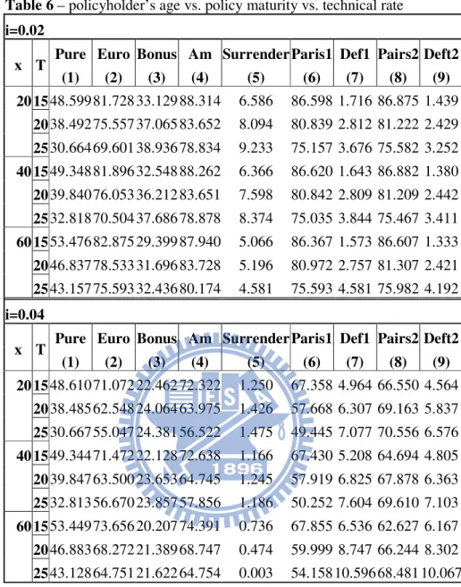
In table 6, we change policyholder’s age and contract maturity. It’s obvious that the surrender value is decreasing against policyholder’s age. Surprisingly, surrender value is increasing against contract maturity if policyholder is young. It is increasing at first and decreasing when contracts maturity is long if policyholder is in middle age. It is decreasing if policyholder is in elder age. The condition changes as we are in different technical rate. We suppose that surrender option is neither strictly increasing nor strictly decreasing against contract maturity. Moreover, we can see default value is increasing either against policyholder’s age or contract maturity.

(29)

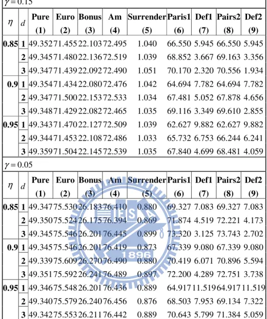
In table 7, we focus on default option value. As we can see, I examine different asset structure toward different insolvency period allowed by bankruptcy law. η is wealth distribution ratio which is also called debt-to asset ratio. As larger as η, as less as equity. We separate the asset structure we examine as follow, sufficient equity capital

(

η =0.85

)

, suitable equity capital

(

η =0.90

)

and inadequate equity capital

(

η =0.95

)

. The default value goes up when equity buffer

(

1−η

)

are low. Comparing with different γ , we can see that default value is higher if target buffer ratio is lower. In considering the bankruptcy law, default value is lower if grace period is longer.

Table 4 – distribution ratio vs. technical rate vs. buffer ratio

0.15

γ =

Pure Euro Bonus Am Surrender Paris1 Def1 Pairs2 Def2

i α (1) (2) (3) (4) (5) (6) (7) (8) (9) 0 0.2 49.350 78.754 29.403 97.564 18.810 97.562 0.002 97.562 0.002 0 100 P = _{0.4 49.348 88.713 39.366 103.919 15.206 103.875 0.044 103.884 0.035} 0.6 49.347 94.526 45.179 108.782 14.256 108.556 0.226 108.622 0.160 0.02 0.2 49.352 69.369 20.016 77.238 7.870 77.179 0.059 77.193 0.045 0 74.510 P = _{0.4 49.347 77.430 28.083 84.087 6.657 83.234 0.853 83.418 0.669} 0.6 49.350 81.896 32.545 88.235 6.339 86.549 1.685 86.820 1.415 0.04 0.2 49.352 61.582 12.230 63.066 1.484 61.159 1.907 61.425 1.641 0 55.865 P = _{0.4 49.348 67.903 18.555 69.063 1.160 65.090 3.973 65.462 3.602} 0.6 49.348 71.475 22.127 72.511 1.036 67.425 5.085 67.829 4.682

(30)

0.10

γ =

i α (1) (2) (3) (4) (5) (6) (7) (8) (9) 0 0.2 49.347 80.396 31.048 98.430 18.034 98.427 0.002 98.428 0.002 0 100 P = _{0.4 49.350 91.032 41.682 105.828 14.796 105.734 0.095 105.761 0.068} 0.6 49.343 97.229 47.886 111.270 14.040 110.845 0.425 110.955 0.315 0.02 0.2 49.353 70.747 21.394 78.227 7.480 78.115 0.113 78.149 0.079 0 74.510 P = _{0.4 49.346 79.381 30.035 85.791 6.410 84.549 1.242 84.785 1.006} 0.6 49.345 84.332 34.987 90.520 6.188 88.320 2.200 88.634 1.886 0.04 0.2 49.343 62.604 13.261 63.989 1.385 61.646 2.343 61.943 2.046 0 55.865 P = _{0.4 49.349 69.510 20.161 70.583 1.073 66.063 4.520 66.448 4.135} 0.6 49.353 73.419 24.066 74.388 0.969 68.790 5.598 69.219 5.169 0.05 γ =

i α (1) (2) (3) (4) (5) (6) (7) (8) (9) 0 0.2 49.350 82.176 32.825 99.502 17.326 99.497 0.005 99.497 0.004 0 100 P = _{0.4 49.348 93.439 44.091 107.971 14.532 107.782 0.189 107.838 0.133} 0.6 49.347 100.055 50.708 114.000 13.945 113.304 0.695 113.464 0.536 0.02 0.2 49.352 72.224 22.872 79.380 7.156 79.162 0.219 79.229 0.151 0 74.510 P = _{0.4 49.347 81.565 32.218 87.821 6.256 86.167 1.654 86.441 1.380} 0.6 49.350 86.766 37.416 92.855 6.088 90.175 2.679 90.529 2.326 0.04 0.2 49.352 63.730 14.379 65.018 1.288 62.263 2.755 62.578 2.440 0 55.865 P = _{0.4 49.348 71.283 21.935 72.276 0.993 67.296 4.980 67.710 4.565} 0.6 49.348 75.552 26.204 76.437 0.885 70.337 6.100 70.814 5.623 Table 5

Different contract type

_Pure_{Euro Bonus Am Surrender Paris1 Def1 Pairs2 Deft2}

Conservative9 49.358 61.577 24.410 63.270 1.693 61.092 2.177 69.098 1.923

Neutral10 49.363 69.525 25.897 70.729 1.204 66.014 4.715 59.446 4.318

Aggressive11 49.353 77.850 25.954 78.760 0.910 71.981 6.780 51.134 6.226

9

Conservative scenario with α=0.2,γ=0.15

10

Neutral scenario with α=0.4,γ =0.10

11

(31)

Table 6 – policyholder’s age vs. policy maturity vs. technical rate i=0.02

Pure Euro Bonus Am Surrender Paris1 Def1 Pairs2 Deft2

x T (1) (2) (3) (4) (5) (6) (7) (8) (9) 20 15 48.599 81.728 33.129 88.314 6.586 86.598 1.716 86.875 1.439 20 38.492 75.557 37.065 83.652 8.094 80.839 2.812 81.222 2.429 25 30.664 69.601 38.936 78.834 9.233 75.157 3.676 75.582 3.252 40 15 49.348 81.896 32.548 88.262 6.366 86.620 1.643 86.882 1.380 20 39.840 76.053 36.212 83.651 7.598 80.842 2.809 81.209 2.442 25 32.818 70.504 37.686 78.878 8.374 75.035 3.844 75.467 3.411 60 15 53.476 82.875 29.399 87.940 5.066 86.367 1.573 86.607 1.333 20 46.837 78.533 31.696 83.728 5.196 80.972 2.757 81.307 2.421 25 43.157 75.593 32.436 80.174 4.581 75.593 4.581 75.982 4.192 i=0.04

Pure Euro Bonus Am Surrender Paris1 Def1 Pairs2 Deft2

x T (1) (2) (3) (4) (5) (6) (7) (8) (9) 20 15 48.610 71.072 22.462 72.322 1.250 67.358 4.964 66.550 4.564 20 38.485 62.548 24.064 63.975 1.426 57.668 6.307 69.163 5.837 25 30.667 55.047 24.381 56.522 1.475 49.445 7.077 70.556 6.576 40 15 49.344 71.472 22.128 72.638 1.166 67.430 5.208 64.694 4.805 20 39.847 63.500 23.653 64.745 1.245 57.919 6.825 67.878 6.363 25 32.813 56.670 23.857 57.856 1.186 50.252 7.604 69.610 7.103 60 15 53.449 73.656 20.207 74.391 0.736 67.855 6.536 62.627 6.167 20 46.883 68.272 21.389 68.747 0.474 59.999 8.747 66.244 8.302 25 43.128 64.751 21.622 64.754 0.003 54.158 10.596 68.481 10.067

(32)

Table 7 – wealth distribution ratio vs. insolvency period vs. buffer ratio

0.15

γ =

η d (1) (2) (3) (4) (5) (6) (7) (8) (9) 0.85 1 49.352 71.455 22.103 72.495 1.040 66.550 5.945 66.550 5.945 2 49.345 71.480 22.136 72.519 1.039 68.852 3.667 69.163 3.356 3 49.347 71.439 22.092 72.490 1.051 70.170 2.320 70.556 1.934 0.9 1 49.354 71.434 22.080 72.476 1.042 64.694 7.782 64.694 7.782 2 49.347 71.500 22.153 72.533 1.034 67.481 5.052 67.878 4.656 3 49.348 71.429 22.082 72.465 1.035 69.116 3.349 69.610 2.855 0.95 1 49.343 71.470 22.127 72.509 1.039 62.627 9.882 62.627 9.882 2 49.344 71.453 22.108 72.486 1.033 65.732 6.753 66.244 6.241 3 49.359 71.504 22.145 72.539 1.035 67.840 4.699 68.481 4.059 0.05 γ =

η d (1) (2) (3) (4) (5) (6) (7) (8) (9) 0.85 1 49.347 75.530 26.183 76.410 0.880 69.327 7.083 69.327 7.083 2 49.350 75.524 26.175 76.394 0.869 71.874 4.519 72.221 4.173 3 49.345 75.546 26.201 76.445 0.899 73.320 3.125 73.743 2.702 0.9 1 49.345 75.546 26.201 76.419 0.873 67.339 9.080 67.339 9.080 2 49.339 75.609 26.270 76.490 0.880 70.419 6.071 70.896 5.594 3 49.351 75.592 26.241 76.489 0.897 72.200 4.289 72.751 3.738 0.95 1 49.346 75.548 26.201 76.436 0.889 64.917 11.519 64.917 11.519 2 49.340 75.579 26.240 76.456 0.876 68.503 7.953 69.134 7.322 3 49.342 75.553 26.211 76.442 0.889 70.643 5.799 71.384 5.059

6 Conclusions

In this paper we have presented a general framework for fair valuation of participating contract combining with insolvency risk and mortality risk. A contract is constructed by pure insurance, bonus option, surrender option and default option. We use the Least Squares Monte Carlo method to calculate the surrender option value. As a practical example, we use endowment insurance to observe the parameter implication. Moreover, we use actual insurance premium to calculate bonus in each years.

(33)

Life insurance companies have traditionally not given much attention to the proper valuation of the various option elements with which their policies have been issued, and this has undoubtedly contributed to the problems now experienced in the life insurance. In considering the asset structure and default option, insurance companies must either have sufficient equity capital or larger target buffer ratio to buffer the unexpected shortfall in the future. With greater distribution ratio of profit or interest rate guarantee in the policy, insurance company need more equity to avoid the insolvency incident happened. Alternatively, to reduce the default value, the insurance company could consider more conservative bonus policies to the extent that this is permitted by law and the contractual terms. In regulation views, if an insurance company is going to sell a competitive contract, supervisory authority must inspect if its capital is sufficient as a buffer or not. In fact, the analysis showed that contract values are highly dependent on the assumed bonus policy and the spread between the market interest rate and the guaranteed rate of interest built into the contract. Some other future research can be considered in the model. First, participating contract is more expensive than pure contract in the practice. However, we only use pure contract value to consider the asset value in our framework. The future research might use the real premium annually to construct the framework. Second, we ignore the fluctuation of mortality in our framework. In practice, insurance company use more conservative interest rate and mortality table to calculate the insurance premium. The surplus in interest rate we’ve already discus in our study. The surplus in mortality spread earning is also distributed in participating contract which is also an extension in the future research. Lastly, our model can be also used in scenario analysis. We can construct an insurance contract portfolio composed by different age. We can use the scenario to arrange a proper asset and liability management to ensure insurance company’s solvency.

(34)

7 Appendix

In this section, we show the regression we use to calculate the continuation value in this analysis. First we note that the backward iteration in step j –

(

, ,

)

( , ) j m l m l j d _{m I} e X τ

∈ is the combination of 3 order of state variable and future life

time and (X_jm l,,τ_dm l, )=

(

r_jm l, ,K_jm l,,Y_jm l,,τ_dm l,

)

with τ_dm l, > . We’ve mentioned the j

reason why we use the polynomial basis function of order 3 in section 3.2. However, since τ_dm l, does not concern with asset value, we only use order 1 in future life time τ_dm l, . In regression terms speaking, we use 19 explanation variable from the combination of (Xm l_j ,,τ_dm l, ) and interception to explain the response variable Cm l_j, . The following equation is the regression function we use in calculating the continuation value of the contracts,

(

)

(

)

(

)

( )

(

)

(

)

(

)

(

)

(

)

(

)

(

( )

)

(

( )

)

(

)

(

)

(

)

2 3 2 3 , , , , , , , 0 1 2 3 4 5 6 2 3 , , , , , , , 7 8 9 10 11 2 2 2 , , , , , , , , 11 12 13 14 2 , , 15 16 m l m l m l m l m l m l m l j j j j j j j m l m l m l m l m l m l m l j j j j j j j m l m l m l m l m l m l m l m l j j j j j j j j m l m l j j C b b Y b Y b Y b r b r b r b K b K b K b r Y b r K b K Y b r Y b r K b S r b S K b K = + + + + + + + + + + × + × + × + × + × + × + × +

(

)

(

)

(

)

2 2 , , , , 17 , , , , 18 19 m l m l m l m l j j j j m l m l m l m l j j j d r b K S b r K S b τ × + × + × × +

All we need in regression constructing is to estimate the 20 parameter above, and then you can have the estimated continuation value of each step. We use this as a signal whether we surrender the contracts or not. Here b i_i, =0,...19 is parameter in regression not the benefit claim. Sorry for the misleading symbol. In fact, there is a bug we need to deal with at j=N₁− , that is 1 m l,

d

τ will be the same for all m∈ . We just cut I_j b at ₁₉ j=N₁− instead. At 1 j= N₁−2,...,1,

(35)

the regression function is ditto. In a much more general form, if τdm l, is the

same for all m∈ , we’ll cut I_j b to run the regression instead in any backward ₁₉

step j.

References

1. Grosen, A. and Jorgensen, P.L., 2000, “Fair Valuation of Life Insurance Liabilities: The Impact of Interest Rate Guarantees, Surrender Options, and Bonus Policies”, Insurance: Mathematics and Economics, 26(1), 37-57. 2. Bacinello, A.R. 2003a, “Fair Valuation of a Guaranteed Life Insurance

Participating Contract Embedding a Surrender Option”, Journal of Risk and

Insurance, Vol. 70, No.3, pp. 461-487.

3. Bacinello, A.R. 2003b, “Pricing Guaranteed Life Insurance Participating Policies with Annual Premiums and Surrender Option”, North American

Actuarial Journal, Jul 2003; 7, 3.

4. Bakshi, G., C. Cao and Z. Chen, 1997, “Empirical performance of alternative option pricing models”, Journal of Finance, vol. 52(5):2003–2049.

5. Melnikov, A., andY. Romaniuk, 2006, “Evaluating the Performance of Gompertz, Makeham and Lee-Carter Mortality Models for Risk Management with Unit-linked Contracts”, Insurance: Mathematics and Economics, 39:310–329.

6. Briys, E., and F. de Varenne, 1994, “Life Insurance in a Contingent Claim Framework: Pricing and Regulatory Implications”, Geneva Papers on Risk

and Insurance Theory, 19(1):53-72.

7. Longstaff, F. A. and Schwartz, E.S., 2001, “Valuing American Options by Simulation: A Simple Least-squares Approach”, The Review of Financial

Studies, vol. 14(1):113–147.

8. Bacinello, A.R., Biffis, E. and Millossovich (2009), “Pricing Life Insurance Contracts with Early Exercise Feature”, Journal of Computational and

(36)

Applied Mathematics, vol. 233(1):27-35

9. Grosen, A., and P.L. Jorgensen, 2002, “Life Insurance Liabilities at Market Value: An analysis of Insolvency Risk, Bonus Policy, and Regulatory Intervention Rules in a Barrier Option Framework”, Journal of Risk and

Insurance, 69(1):63-91.

10. Jensen, B., Jorgensen, P.L. and Grosen A., 2001, “Finite Difference Approach to the Valuation of Path Dependent Life Insurance Liabilities”,

Geneva Papers on Risk and Insurance Theory, 26(1):57-84.

11. Cox, J.C., Ingersoll, J.E. and Ross, S.A., “A Theory of the Term Structure of Interest Rates”, Econometrica, 53(1985):385-497.

12. Chen A., Suchanecki, M., 2007, “Default Risk, Bankruptcy procedures and the market value of life insurance liabilities”, Insurance: Mathematics and

Econometrics 40(2007):231-255.

13. Smith, M. L., 1982, “The life insurance policy as an options package”. The

考量破產風險後分紅保單在保險公司的負債評價

國

立

交

通

大

學

財務金融研究所

碩

碩

碩

碩

士

士

士

士

論

論

論

論

文

文

文

文