單載波調變與多天線輸入多天線輸出傳輸技術應用於60 GHz光載微波無線訊號系統

(1)

國立交通大學

顯示科技研究所

碩士論文

單載波調變與多天線輸入多天線輸出傳輸

技術應用於 60 GHz 光載微波無線訊號系統

Multiple-Input Multiple-Output Technology in

60 GHz Radio-over-Fiber System with

Single Carrier Modulation

研究生：李維元

指導教授：陳智弘教授

(2)

i

Multiple-Input Multiple-Output Technology in

60 GHz Radio-over-Fiber System with

Single Carrier Modulation

研究生: 李維元 Student: Wei-Yuan Lee

指導教授: 陳智弘 advisor: Jye-Hong Chen

國立交通大學

顯示科技研究所

碩士論文

Thesis submitted to the Display Institute

College of Electrical Engineering and Computer Science National Chiao Tung University

in partial fulfillment of the requirements for the degree of Master in Display Institute

(3)

ii

Acknowledgments

時光匆匆，一眨眼，兩年的碩士班生涯已經接近尾聲，這一路走來沒有特別的驚濤駭浪，沒有大起大落的電影情節，一路走得十分踏實，按部就班的完成每一個目標，能走的這麼順利，需要感謝的人實在是太多了，首先感謝我的指導教授陳智弘老師，不僅提供完善的學習環境和實驗設備，也讓我學習到許多待人處事原則，更使我對於 ”學習 ”這兩個字有更深刻的體悟。由衷的感謝林俊廷老師總在我學習的路上提點一盞明燈，和老師的討論之中也學習到非常多研究的方法與對實驗的態度，使得論文能順利完成。令外，也非常感謝魏嘉建老師在我研究所生涯中對我的幫助。特別的感謝施伯宗學長、江文智學長以及陳星宇學長在實驗上以及程式上對我的幫助，不厭其煩的指導與幫忙讓我節省了許多摸索的時間。再來還要感謝實驗室的同學們宜旻、冠穎、上詠、明義及俊鴻，與他們的相處，讓碩班生活更加豐富與充實。也十分感謝學弟妹致勻、宗紘、威爾、勁威、頊宸、信豪、志傑、厚茨與乃慧等人的幫忙。也謝謝所有曾經幫助過我的人，謝謝你們。最後要謝謝我的父母與家人，能給我一個衣食無缺的環境，讓我能全心全意的完成碩士學業，你們的支持是我前進的動力。另一段旅程即將展開，但是我永遠也不會忘記我在交大所經歷過、感受過、學習過的一切，謝謝你交大! 再會了交大!

(4)

iii

多天線輸入多天線輸出傳輸技術應用於

60 GHz 光載微波無線訊號系統

學生: 李維元指導教授: 陳智弘教授國立交通大學顯示科技研究所碩士班

摘要

互動式多媒體的快速發展，導致新的無線網路服務不斷推陳出新，對於傳輸速度的要求也逐漸升高，帶動了 multi-Gbps 無線傳輸技術的發展。然而，60 GHz 的免授權頻段其頻寬限制在 7 GHz，並且 60 GHz 的微波訊號在空氣中有著非常大的衰減，較適合短距離的無線傳輸。因此，60 GHz 的光載微波無線訊號系統搭配上空間多功的 MIMO 技術是一個非常可實現的一個方法，提供一個寬頻、覆蓋範圍廣以及機動性兼具的服務。在此篇論文中，藉由頻域等化器實現 2 x 2 MIMO 技術，提高頻譜使用效率達成傳輸資料倍增的效果。我們在實驗上成功傳輸 60GHz 頻段上 7 GHz 免授權頻寬的 16-QAM MIMO 單載波訊號，傳輸速度達到 2 x 13.575 Gb/s，在經過 25 公里的單模光纖和 3 公尺的無線傳輸以後，訊號品質幾乎沒有改變。

(5)

iv

60 GHz Radio-over-Fiber System with

Multiple-Input Multiple-Output Technology

Student: Wei-Yuan Lee Advisor: Dr. Jye-Hong Chen

Display Institute, National Chiao Tung University

Abstract

The rapid growth of data rates of new wireless applications led by interactive multimedia services is driving the need for multi-Gbps wireless communication technologies in the near future. However, the bandwidth of the license free spectrum at 60 GHz is limit to 7 GHz and 60-GHz

millimeter-waves have very high propagation losses rendering them more suitable for short-range wireless links (~10m). Therefore, 60-GHz

radio-over-fiber (RoF) system with spatial-multiplexing MIMO technology is a promising candidate to provide broadband service, wide coverage, and

mobility.

In this these, 2 x 2 MIMO technique is realized by frequency domain equalizer (FDE) to improve spectrum efficiency doubling the data throughput. We experimentally demonstrate 2 x 13.575 Gb/s 16-QAM MIMO single carrier signal transmission within 7-GHz license-free bandwidth at 60-GHz band. The power penalty is negligible after transmission over 25-km single mode fiber and 3m wireless distance.

(6)

v

List of Figures

Figure 1-1 The allocated band and bandwidth in the U.S.A. ... 2

Figure 2-1 the concept of RoF system with MIMO technology.. ... 5

Figure 2-2 time diversity.. ... 7

Figure 2-3 2x1 MISO. ... 8

Figure 2-4 2x1 Alamouti space-time code.. ... 10

Figure 2-5 simulation result of Alamouti space-time code... ... 10

Figure 2-6 MIMO channel converts into parallel channel.. ... 12

Figure 2-7 2x2 spatial multiplexing MIMO... 14

Figure 2-8 the correlated channel. ... 15

Figure 2-9 simulation result of MIMO with ZF receiver.. ... 15

Figure 2-10 simulation result of MIMO with ML receiver.. ... 17

Figure 3-1 the basic ideal of FDE.. ... 22

Figure 3-2 the block diagram of FDE. ... 22

Figure 3-3 2x2 MIMO RoF system.. ... 23

Figure 3-4 the block diagram of 2x2 MIMO with FDE.. ... 24

Figure 4-1 Single-electrode Mach-Zehnder Modulator.. ... 28

Figure 4-2 the different order of Bessel function versus m.. ... 29

Figure 4-3 the concept of the proposed system.. ... 32

Figure 4-4 Magnitude of Bessel functions versus different modulation index.. ... 34

Figure 5-1 experimental setup of the propose system.. ... 37

Figure 5-2 optical spectrum for 16 QAM SC signal.. ... 37

Figure 5-3 electrical spectrum for 16 QAM SC signal.. ... 38

Figure 5-4 BER curve of QPSK SC signal with SISO channel... ... 39

Figure 5-5 Constellations of the QPSK SC signal with SISO channel.. ... 39

(9)

viii

Figure 5-7 Constellations of the 8-QAM SC signal with SISO channel.. ... 41

Figure 5-8 BER curve of 16-QAM SC signal with SISO channel.. ... 41

Figure 5-9 Constellations of the 8-QAM SC signal with SISO channel.. ... 42

Figure 5-10 BER curve of 16-QAM SC signal with MIMO channel in BTB transmission at different FFT size... ... 43

Figure 5-11 BER curve of 16-QAM SC signal with MIMO channel in BTB transmission at different CP length.. ... 44

Figure 5-12 SNR versus MIMO Channel correlation of 16-QAM SC signal in BTB transmission.. ... 45

Figure 5-13 BER curve of QPSK SC signal with MIMO channel.. ... 46

Figure 5-14 Constellations of the QPSK MIMO signal.. ... 47

Figure 5-15 BER curve of 8-QAM SC signal with MIMO channel.. ... 48

Figure 5-16 Constellations of the 8-QAM MIMO signal... ... 48

Figure 5-17 BER curve of 16-QAM SC signal with MIMO channel.. ... 49

(10)

1

Chapter 1 Introduction

1.1 Background

With the rapid growth of technology, people have been from computer generation to the internet generation. Many kinds of internet products, such as smart phone, tablet PC, and various internet services, like facebook, twitter, high-definition images, are developed rapidly in the recent years. Peoples’ life and internet have been combined closely. People need the internet everywhere, even on the bus, on the train, on the way to somewhere. Thus, the wireless communication becomes more and more important today.

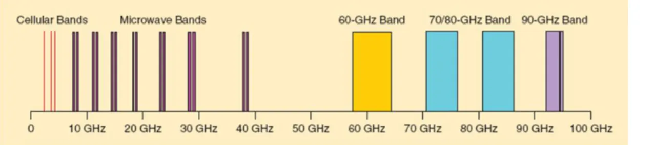
In order to support such internet services, the speed of data transmission must improve. However, the most popular communication standards, such as 3G, 4G and WiFi don’t have enough commercial wireless communication bandwidth, and the data rate can’t exceed 1Gbit/s. The carrier frequency of the wireless signal has to be raised to break the limitation of bandwidth. The allocation of communication band and bandwidth are different from different countries, and Figure 1-1 shows that the band and the bandwidth are allowed to use in the USA. After U.S. Federal Communications opened bands with 50-120 GHz, there are several bands above 50GHz which have large enough

bandwidths to support high-speed data transmission (57-64GHz, 71-76GHz, 81-86GHz and 92-95GHz). And the band at 60 GHz which have 7 GHz unlicensed bandwidth is attractive to the industry and the research [1-3].

(11)

2

Due to the physical property of the transmission wave, the transmission distance will decrease when the carrier frequency increase. Because of the smaller coverage area, we need more base stations than using lower carrier frequency to support the same service region. The signal loss will be the main problem when high-frequency signal is transmitted by the coaxial cable, and second problem is the cost issue that the price of high-frequency coaxial cable is very high. Thus, Radio-over-Fiber (RoF) system [4] was proposed to solve the power and cost issues in the millimeter-wave signals.

Using fiber as the transmission medium is one of the best solution

because there is not only unlimited bandwidth but also less power loss in fiber. RoF system can save the system cost by reducing the equipment of base

stations (BSs) along with highly centralized central station (CS) equipped with optical and mm-wave components.

1.2 Motivation

Due to the demand for higher bandwidth, MIMO technology [5-7] becomes the most attractive solution to increase the bandwidth efficiency. Thus, MIMO technology has been used in many communication standards for recent years. Table 1-1 [8] shows various wireless communication standards,

(12)

3

and several standards such as WiMax, LTE, WiFi and so on, have involved MIMO technology. Hence, MIMO transmission technology will play an important role to the development of the wireless communication in the future.

Standard Family Primary Use Radio Tech Downlink (Mbit/s) Uplink (Mbit/s)

WiMAX 802.16 Mobile Internet MIMO-SOFDMA 128 (in 20MHz bandwidth)

56 (in 20MHz bandwidth)

LTE UMTS/4GSM General 4G OFDMA/MIMO/S C-FDMA 100 (in 20MHz bandwidth) 50 (in 20 MHz bandwidth) Mobile Internet 5.3 1.8 mobility up to 200mph (350km/h) 10.6 3.6 15.9 5.4

HIPERMAN HIPERMAN Mobile Internet OFDM

Wi-Fi 802.11(11n) Mobile Internet OFDM/MIMO

EDGE Evolution GSM Mobile Internet TDMA/FDD 1.6 0.5

CDMA/FDD 0.384 0.384

14.4 5.76

CDMA/FDD/MIMO 56 22

UMTS-TDD UMTS/3GSM Mobile Internet CDMA/TDD 1xRTT CDMA2000 Mobile phone CDMA

EV-DO 1x Rev. 0 EV-DO 1x Rev.A EV-DO Rev.B

CDMA2000 Mobile Internet CDMA/FDD

2.45 3.1 4.9xN 0.15 1.8 1.8xN 36 UMTS W-CDMA HSDPA+HSUPA HSPA+ UMTS/3GSM General 3G 16 0.144

Flash-OFDM Flash-OFDM Flash-OFDM

56.9

300 (using 4x4 configuration in 20MHz bandwidth) or 600 (using 4x4 configuration in

40MHz bandwidth)

iBurst 802.2 Mobile Internet

HC-SDMA/TDD/MIMO 95

(13)

4

1.3 Objection and Problem Statement

In this thesis, we will demonstrate the 60 GHz RoF system using 2 x 2 MIMO technology transmitting the Single Carrier vector signal to increase the spectrum efficiency in the 7 GHz unlicensed band. However, there are two main problems we will meet.

The first challenge is non-flat channel response with up to 10dB deviation within the 7 GHz spectrum. The 7 GHz SC signal will have a serious ISI problem. The complexity of the MIMO process in the time domain will rapidly increase. To overcome this problem, the SC frequency domain

equalizer (FDE) [9] is used. FDE not only can compensate the uneven channel response but also can well separate the MIMO signals in the frequency

domain.

The second one is the noise enhancement because of MIMO channel correlation. Channel correlation between different transmitted antennas is very important to the signal performance in the light of sight (LOS) MIMO

scenario. The channel correlation is related to the distance and the angles of received signals. The problem can be solved by increasing the antenna pairs or introducing the concept of the smart antennas where we don’t focus on this topic in this thesis. The channel correlation can also be decreased by well adjusting the antenna spacing.

(14)

5

Chapter 2 Multiple-Input Multiple-Output (MIMO)

Technology

2.1 Preface

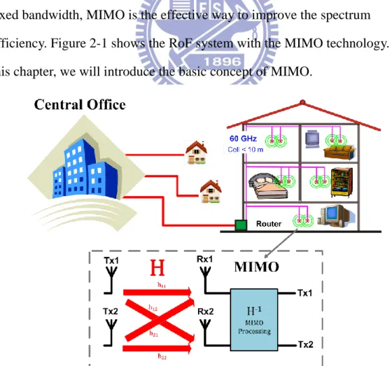
The RoF system is the possible solution of the high data rate wireless transmission in the future because of the property of the fiber which is low loss and have almost unlimited bandwidth. However, the bandwidth in wireless communication is constrained by the law. In order to raise the data rate in the fixed bandwidth, MIMO is the effective way to improve the spectrum

efficiency. Figure 2-1 shows the RoF system with the MIMO technology. In this chapter, we will introduce the basic concept of MIMO.

(15)

6

2.2 MIMO Technology for Improving Performance 2.2.1 Diversity

In the non-LOS wireless communication, we don’t know how the signal is received form transmitter to the receiver. The signal may be reflected, scattered, refracted and even blocked on the way to the receiver. If the signal performance is so poor that can’t be the reliable communication, we call this path is in a deep fade. When the path is in a deep fade, the communication will suffer from errors. A technique is called diversity, and it can significantly improve the performance over the fading channels.

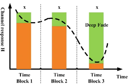
There are many ways to obtain diversity, we introduce three diversity techniques in time, frequency and space in the chapter. Figure 2-2 shows the concept of the time diversity. H is a fading channel variously with time. When the time block 3 is in a deep fade, the signal at time block3 will suffer from error. Now, the same signal x is transmitted three times. Thus, even if the time block 3 is in deep fade, the signal x still could be detected correctly depending the received signals at other two time blocks. Similarly, one can also exploit diversity over frequency if the channel is frequency-selective which means the channel changes variously with the frequency. Multiple transmit and receive antennas will create the different channels from the different transmit antennas to receive antennas. The same signal can be received many times because of the different transmit paths, and the spatial diversity is obtained. The diversity technique is an important resource to the wireless communication, and we will introduce the Alamouti space-time code to implement the space diversity to improve the signal performance in next section.

(16)

7

2.2.2 Alamouti Space-Time Code

Spatial diversity which we can also call it antenna diversity, it involves both the receive diversity, using multiple receive antennas (single input multiple output, SIMO channels), and the transmit diversity, using multiple transmit antennas (multiple input single output, MISO channels). Channels with multiple transmit antennas and multiple receive antennas (multiple input multiple output, MIMO channels) provide more potential.

Alamouti scheme was proposed by Mr. Siavash M Alamouti in his landmark paper – A Simple Transmit Diversity Technique for Wireless Communication. This is the transmit diversity scheme proposed in several third-generation cellular standards. The Alamouti scheme is designed for two transmit antennas at the first, but more than two transmit antennas is possible. For the discussion, we will assume that the channel is a flat fading Rayleigh multipath channel.

Figure 2-3 shows a 2 x 1 MISO scenario, and there are two transmit antennas and one receive antenna. Two transmitted signals x1 and x2 are

(17)

8

transmitted to the receive antenna and the received signal y is written as

𝑦,m- = ℎ₁,𝑚-𝑥₁,𝑚- + ℎ₂,𝑚-𝑥₂,𝑚- + 𝑤,𝑚- (Eq. 2-1) Where h_i is the channel gain from transmit antenna i, and w is the additive white Gaussian noise (AWGN).

Now, we have a transmission sequence such as {u₁, u₂, u₃, u₄, …} which are the data symbols. In the normal transmission, we will transmit u1 in the first

time slot, u₂in the second time slot, u₃ in the third time slot and so on. However, The Alamouti scheme transmits two symbols u1 and u2 over two times. At time

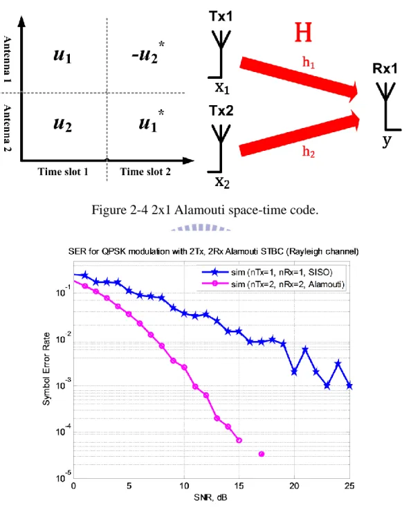
slot 1, x₁[1] = u₁, x₂[1] = u₂; At time slot 2, x₁[2] = -u₂*, x₂[2] = u₁*; We assume that the channel remain constant over the two symbol times which h1 = h1[1] =

h₁[2], h₂= h₂[1] = h₂[2], as the figure 2-4 shown, 2 x 1 Alamouti space-time code. Then, the receive signal can be expressed as

,𝑦,1- 𝑦,2-- = ,ℎ1 ℎ2- [𝑢1 −𝑢2 ∗

𝑢₂ 𝑢₁∗ ] + ,𝑤,1- 𝑤,2-- (Eq. 2-2)

The equation can be rewrote as

(18)

9 [_𝑦,2-𝑦,1-_∗] = [ℎ_ℎ1 ℎ2 2 ∗ _−ℎ 1∗] [ 𝑢1 𝑢2] + [𝑤,1-𝑤,2-∗] (Eq. 2-3) Let us define H = [ℎ_ℎ1 ℎ2 2∗ −ℎ1∗] (Eq. 2-4)

The channel coefficients h₁, h₂ have known. To solve for u₁, u₂, we multiple the Hermitian matrix of H to the [y[1] y[2]*]T

H𝐻 _{= [}ℎ1∗ ℎ2 ℎ2∗ −ℎ1 ] (Eq. 2-5) [𝑟_𝑟1 2] = H 𝐻_[ 𝑦,1-𝑦,2-∗] = [ ℎ₁∗ _ℎ 2 ℎ₂∗ _−ℎ 1 ] [ ℎ₁ ℎ₂ ℎ₂∗ _−ℎ 1∗] [ 𝑢₁ 𝑢₂] + H𝐻[𝑤_𝑤,2-,1-∗] (Eq. 2-6) [𝑟_𝑟1 2] = [ |ℎ1|2+ |ℎ2|2 0 0 |ℎ₁|2_{+ |ℎ} 2|2] [ 𝑢1 𝑢2] + H 𝐻_[𝑤 ,1-𝑤,2-∗] (Eq. 2-7)

The estimate of transmit symbols are by inversing the diagonal matrix

(H𝐻_H)−1 _{= [} 1 |ℎ1|2+|ℎ2|2 0 0 _|ℎ 1 1|2+|ℎ2|2 ] (Eq. 2-8) [𝑢̂_𝑢̂1 2] = (H 𝐻_H)−1_[𝑟1 𝑟₂] + (H𝐻H)−1H𝐻[𝑤_𝑤,2-,1-∗] (Eq. 2-9) [𝑢̂_𝑢̂1 2] = [ 𝑢1 𝑢2] + (H 𝐻_H)−1_H𝐻_[𝑤 ,1-𝑤,2-∗] (Eq. 2-10)

Thus, the transmit diversity gain is 2 for the detection of each symbol. It is possible to provide diversity order 2M with two transmit and M receive

(19)

10

the channel is the flat fading Rayleigh channel, and the noise is AWGN. Clearly, 2 x 2 Alamouti scheme has better performance than the SISO channel.

2.3 MIMO Technology for Improving Capacity

We will see that under suitable channel conditions, MIMO channel provides an additional spatial dimension for communication and degrees of

Figure 2-4 2x1 Alamouti space-time code.

(20)

11

freedom. These additional degrees of freedom can be exploited by spatial multiplexing several data streams on to the MIMO channel and the overall capacity is increased.

The time-invariant MIMO channel with n_t transmit and n_r receive antennas can be written as the nr by nt deterministic matrix H

𝐲 = 𝐇𝐱 + 𝐰 (Eq. 2-11) where x, y and w denote the transmitted signal, received signal and white

Gaussian noise at a symbol time.

This is a vector Gaussian channel. The capacity can be computed by decomposing the vector channel into a set of parallel, independent scalar Gaussian sub-channels. The matrix H has a singular value decomposition (SVD):

𝐇 = 𝐔𝛔𝐕𝐻_{(Eq. 2-12)}

where U and V are unitary matrices and σ is a rectangular matrix whose diagonal elements are non-negative real numbers. The diagonal elements λ1 ≥ λ2 ≥ … ≥ λnmin are the ordered singular values of matrix H,

where nmim: = min (nt, nr). We can rewrite the SVD as

𝐇 = ∑ 𝜆𝑖𝐮𝑖𝐯𝑖𝐻 𝑛𝑚𝑖𝑛

𝑖=1

(Eq. 2-13) The sum of rank-one matrices λiuiviH. It can be seen that the rank of H is the number of non-zero singular values.

If we define

𝐱̃ = 𝐕𝐻_{𝐱 (Eq. 2-14)}

(21)

12

𝐰̃ = 𝐔𝐻_{𝒘 (Eq. 2-16)}

then we can rewrite the channel as

𝐲̃ = 𝛔𝐱̃ + 𝐰̃ (Eq. 2-17)

Then, we have an equivalent representation as parallel Gaussian channel

𝑦̃_𝑖 = 𝜆_𝑖𝑥̃_𝑖+ 𝑤̃_𝑖, 𝑖 = 1,2, … , n_𝑚𝑖𝑛 (Eq. 2-18) Figure 2-6 shows the equivalence.

We can look the SVD decomposition as two coordinate transformations. If the input is expressed in terms of coordinate system defined by the columns of V and the output is expressed in terms of a coordinate system defined by the column U, then the relationship between input and output can be very simple. Thus, the property of MIMO channel will dominate how much data we can transmit.

在這裡鍵入方程式。

2.3.1 Spatial Multiplexing : Zero-Forcing Receiver

For a deterministic time-invariant MIMO channel, the capacity-achieving architecture is simple. Independent data streams are multiplexed in an

appropriate coordinate system. The receiver transforms the received vector into Figure 2-6 MIMO channel converts into parallel channel.

𝐱

(22)

13

another appropriate coordinate system to separate the different data streams. Figure 2-7 shows a 2 x2 spatial multiplexing MIMO scheme. Let’s rewrite it to the matrix form as:

𝐲 = 𝐇𝐱 + 𝐰 (Eq. 2-19) [y_y1 2] = [ ℎ11 ℎ21 ℎ₁₂ ℎ₂₂] [ x1 x2] + [ w1 w2] (Eq. 2-20)

where H is the channel matrix, and x = [x1 x2]T is the input vector is consist of

two independent symbols x₁, x₂, w = [w₁ w₂]T is the noise. Assume the element of the channel matrix is known, the transmitted data can be recovered by using the zero-forcing algorithm and written as

𝐲̃ = 𝐇−1_{𝐲 = 𝐱 + 𝐇}−1_{𝐰 = 𝐱 + 𝐰}_{̃ (Eq. 2-21)}

However, the noise w̃₁ and w̃₂ are correlated. The performance will decrease. First, we focus on the detection of symbol form transmit antenna 1. The noise become:

w̃₁ = ℎ22w1− ℎ21w2 ℎ11ℎ22− ℎ12ℎ21

(Eq. 2-22) Because of the white noise w₁ and w₂ have the same power, the noise w̃₁ can be expressed as

w̃₁ =√|ℎ21|2+ |ℎ22|2 ℎ11ℎ22− ℎ12ℎ21 𝑧1

(Eq. 2-23) where z1 is white noise and the power is as same as w1 and w2. Thus, we rewrite

(23)

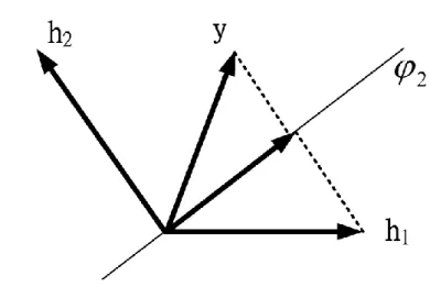
14 ỹ1 = x1+ √|ℎ₂₁|2_{+ |ℎ} 22|2 ℎ₁₁ℎ₂₂− ℎ₁₂ℎ₂₁ 𝑧1 (Eq. 2-24) Then we define y₁′ ₌ ℎ11ℎ22− ℎ12ℎ21 √|ℎ₂₁|2_{+ |ℎ} 22|2 ỹ1 = (𝜙2𝐻𝐡1)x1+ 𝑧1 (Eq. 2-25) where 𝐡₁ = [ℎ_ℎ11 12] , 𝜙2 = 1 √|ℎ21|2+ |ℎ22|2 [_−ℎ ℎ22∗ 21∗ ] (Eq. 2-26) The h₁ can be seen as the direction of the signal from transmit antenna 1, and the ϕ2 is the direction orthogonal to h2. Equation 2-25 represents that the signal

form transmit antenna 1 is detected by projecting the received signal y to the direction perpendicular to the direction of the transmit antenna 2, h2. Hence,

the interference from transmit antenna 2 can be eliminated. However, if the h₁ and h2 are not orthogonal in the beginning, the vector of h1 orthogonal to the h2

will be smaller than h₁ itself as figure 2-8 shown.

(24)

15

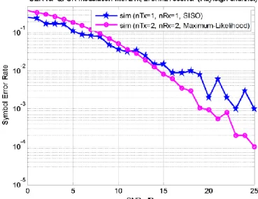
Figure 2-9 is the simulation result of 2x2 MIMO channel with

Zero-Forcing receiver where the channel is the flat fading Rayleigh channel, and the noise is AWGN and the transmit antennas transmit two independent symbols at once. We only use the one dimension to decode the signal by the projection, so we don’t have any diversity gain in this scheme. Thus, the performance is not better to the SISO channel, but the capacity is double.

Figure 2-8 the correlated channel.

(25)

16

2.3.2 Spatial Multiplexing : Maximum-Likelihood Receiver

Maximum-Likelihood (ML) receiver is the very directly way to detect the independent data streams. The core idea of the ML detection is to compare all of the possible transmitted symbols to find the maximum likely one. Figure 2-7 is the 2x2 spatial multiplexing MIMO scheme. Equation 2-19 and Equation 2-20 is the matrix form of this scheme, where H is the channel matrix, and x = [x1 x2]T is the input vector is consist of two independent symbols x1, x2, w =

[w₁ w₂]T is white noise. The ML detection bases on the following equation: 𝐬 = arg minx‖𝐲 − 𝐇𝐱̂‖2 (Eq. 2-27)

Assume the channel matrix H is known, and we also know what kind of the symbol 𝐱̂ the transmit antenna may sent. Then, the receiver can decision what kind of symbol it is.

For an example, the 2x2 MIMO scheme is like figure 2-7, and the modulation is BPSK. The ML receiver tries to find 𝐱̂ which minimizes 𝐊 = ‖𝐲 − 𝐇𝐱̂‖2_{, and the possible value of the BPSK symbol is +1 or -1. So we need}

to find the minimum from all four possible combinations. 𝐊_+1,+1 = ‖[_yy1 2] − [ ℎ11 ℎ21 ℎ₁₂ ℎ₂₂] [+1+1]‖ 2 (Eq. 2-28) 𝐊_+1,−1 = ‖[_yy1 2] − [ ℎ11 ℎ21 ℎ₁₂ ℎ₂₂] [+1−1]‖ 2 (Eq. 2-29) 𝐊_−1,+1 = ‖[_yy1 2] − [ ℎ11 ℎ21 ℎ₁₂ ℎ₂₂] [−1+1]‖ 2 (Eq. 2-30) 𝐊_−1,−1 = ‖[_yy1 2] − [ ℎ11 ℎ21 ℎ₁₂ ℎ₂₂] [−1−1]‖ 2 (Eq. 2-31) If the minimum is K+1,+1, the estimate transmitted symbol 𝐱̂ is [+1,+1]. Due to

all of the dimensions are considered, the performance is better than the SISO channel by the diversity gain. Figure 2-10 shows the simulation result. However, the complexity of the ML receiver will exponentially grow with

(26)

17

increasing the number of antennas and the order of data format of symbols.

(27)

18

Chapter 3 Single Carrier Frequency Domain Equalizer

3.1 Preface

In this thesis, we want to apply the MIMO antenna technology to the 60 GHz RoF system with 7 GHz broadband bandwidth doubling the data rate. However, such high carrier frequency signal (60 GHz) has very high propagation losses rendering it more suitable for short-range wireless links (~10m). The wideband 60 GHz RoF system has an uneven frequency

response of up to 12 dB within 7 GHz license-free band. These two properties make the MIMO channel in 60 GHz RoF system is a time-invariant and frequency-selective channel. Hence, it is the different situation from the assumption in the chapter 2. We assume the MIMO channel is a flat fading Rayleigh channel in the chapter 2. In this chapter, the complexity will highly increase by using the ZF detector due to the frequency-selective channel, but we will introduce the frequency domain equalizer (FDE) to MIMO

technology which is simple method to double the data rate.

3.2 Inter-Symbol Interference

Inter-symbol interference is an important issue in digital communication. It is a form of distortion of signal where the symbols interfere to the symbols each other. That’s just like the noise to the decision samples, and that will make the communication less reliable. ISI usually comes from two different situations. One is the multipath propagation, and the other one is the uneven

(28)

19

frequency response of the system.

ISI of the multipath propagation occurs because of the wireless signal from the transmit antenna to the receive antenna via different paths. The same signal will arrive to the receiver at different time due to the various paths, so the signals are going to distort the amplitude and phase which cause

interference between symbols at different time. The phenomenon of fiber dispersion also results in ISI. The reason is similar to the multipath propagation.

Compared to the ISI of the multipath propagation, the ISI because of the uneven frequency response of the system is presented in both wired and wireless communication. Every component in the communication system has its own frequency response, so the frequency response of the entire system is non-flat and will cause ISI.

3.3 Linear Convolution and Circular Convolution

The concept of the circular convolution plays an important role to the SC FDE. In this section, we will introduce form the linear convolution to the circular convolution [11].

The linear convolution of two sequences x1[n] of N1-point and x2[n] of

N₂-point is given by x3,n- = x1,n- ∗ x2,n- = ∑ x1 ,k-∞ 𝑘=−∞ x2,n − k- = ∑ x1 ,k-𝑁1−1 𝑘=0 x2,n − k- (Eq. 3-1) where x₃[n] is a (N₁ + N₂ - 1)-point sequence. Now, the same sequences x₁[n] and x2[n], and we choose N = max (N1, N2) to compute the N-point circular

(29)

20 convolution x4,n- = x1,n- ⨂ x2,n- = ∑ x1 ,m-𝑁−1 𝑚=0 x2(,n − m-)𝑁 (Eq. 3-2) where x₄,n- is a N-point sequence. Assume we choose N = (N1 + N2 –

1)-point to do the circular convolution, x₄,n- becomes x₄,n- = x₁,n- ⨂ x₂,n- = ∑ x₁ ,m-𝑁−1 𝑚=0 x₂(,n − m-)_𝑁 = ∑ x₁,m- ∑ x₂,n − m − rN-∞ 𝑟=−∞ 𝑁−1 𝑚=0 = ∑ ∑ x₁,m-x₂,n − m − rN-𝑁−1 𝑚=0 ∞ 𝑟=−∞ = ∑ x3,n − rN-∞ 𝑟=−∞ (Eq. 3-3) Then x4,n- = x3,n- 0 ≤ 𝑛 ≤ 𝑁 − 1 (Eq. 3-4)

Thus, the circular convolution is the aliased version of the linear convolution. On the other hand, if we pad the number of zeros to make x₁,n- and x₂,n- become a (N₁ + N₂ – 1)-point sequence, the result of circular convolution is equal to the result of linear convolution.

3.4 Single Carrier Frequency Domain Equalizer

The traditional method to compensate for ISI is to use a time domain equalizer at the receiver. One or more transversal filters are main components

(30)

21

where the number of adaptive tap coefficients is on the order of number of the data symbols spanned by ISI. An SC system transmits a single carrier

modulated with QAM at high symbol rate suffering a serious ISI problem. The complexity and digital processing speed become exorbitant, and the time domain equalizer becomes unattractive.

Frequency domain equalizer compensates the channel response in the frequency domain. Figure 3-1 shows the basic idea of FDE. When a signal x into the system which the channel impulse response is h, we know that it is the convolution of the signal x and the channel h in the time domain. The

convolution process becomes the simple multiplication in the frequency

domain where F{} and F-1{} are the fast Fourier transform and inverse Fourier transform, and we can easily use one tap equalizer to compensate the signal in the frequency domain. For channel with severe ISI, frequency domain

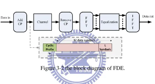
equalization is computationally simpler than the time domain equalizer. Figure 3-2 is the block diagram of FDE. At first, the received signal passes the fast Fourier transform (FFT) operation transforming the time domain SC signal to frequency domain, and then the compensated signal transfer to the time domain signal by inverse fast Fourier transform (IFFT) after equalization. However, we can’t do FFT to all of the data and process all of the data at once, because the memory of the digital circuit has its limitation. Thus, we want to process the signal in the block form which every M symbols (M = 64, 128, 256… and so on) a block. Then, the concept of cyclic prefix (CP) is introduced. CP length is L symbols which is added form the end of the data block and the length of data block becomes M + L symbols at transmitter. CP makes every data block

(31)

22

M symbols at receiver after removing CP.

Figure 3-1 the basic ideal of FDE.

3.5 MIMO Technology with Frequency Domain Equalizer

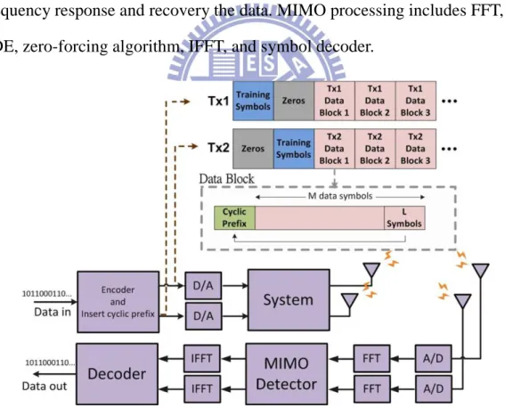
Figure 3-3 shows the fundamental concept of 2 x 2 MIMO RoF System. Two antennas, Tx1 and Tx2, transmit two different signals to the receive

antennas, Rx1 and Rx2. The receive signals will be the summation of these two transmitted signals with different channel coefficient s due to the different transmitting paths and can be expressed as

[y_y1 2] = [ ℎ₁₁ ℎ₂₁ ℎ₁₂ ℎ₂₂] [ x₁ x₂] + [ww1₂] (Eq. 3-5) where y and x are received and transmitted data, respectively, w is the noise, and h is the channel coefficient. If the channel coefficient is estimated by appropriate training symbol, the transmitted data can be recovered by using the

Channel Time domain Frequency domain Fourier transform

x

_h

y

y = h * x F{y} = F{h}·F{x} F{x} = F{h}-1·F{y}

(32)

23

zero-forcing algorithm and written as [x̂1 x̂₂] = [ ℎ₁₁ ℎ₂₁ ℎ12 ℎ22] −1 [y_y1 2] (Eq. 3-6)

However, since 60 GHz RoF system has uneven frequency response of up to 12 dB within 7 GHz license-free band, the system would encounter the serious inter-symbol interference (ISI) problem. The complexity of MIMO processing in the time domain would significantly increase with the number of signal taps causing by ISI. Thus, we want to find a suitable way avoiding the highly complex matrix calculation. The proper answer is the FDE, and the received signal y transformed to the frequency domain by FFT can be expressed as

[𝐹*y_𝐹*y1,𝑚-+ 2,𝑚-+] = [ 𝐹*ℎ11,𝑚-+ 𝐹*ℎ21,𝑚-+ 𝐹*ℎ₁₂,𝑚-+ 𝐹*ℎ₂₂,𝑚-+] [ 𝐹*x1,𝑚-+ 𝐹*x₂,𝑚-+] + [ 𝐹*w1,𝑚-+ 𝐹*w₂,𝑚-+] 𝑚 = 0,1, … , 𝑀 − 1 (Eq. 3-7) Every M received symbols transform to the frequency domain by FFT. As same as the previous mentioned, the transmitted data can be recovered by using the zero-forcing algorithm, if the channel coefficients in frequency domain are estimated. [𝐹*x̂_𝐹*x̂1,𝑚-+ 2,𝑚-+] = [ 𝐹*ℎ₁₁,𝑚-+ 𝐹*ℎ₂₁,𝑚-+ 𝐹*ℎ₁₂,𝑚-+ 𝐹*ℎ₂₂,𝑚-+] −1 [𝐹*y_𝐹*y1,𝑚-+ 2,𝑚-+] 𝑚 = 0,1, … , 𝑀 − 1 (Eq. 3-8) Figure 3-3 2x2 MIMO RoF system.

(33)

24

By using the inverse fast Fourier transform F-1{}, we can get the transmitted signals in the time domain and can be expressed as

x̂_𝑖,m- = 𝐹−1_{𝐹*x̂

𝑖,m-+} 𝑖 = 1,2 (Eq. 3-9)

Figure 3-4 shows the block diagram for 2 x 2 MIMO systems with FDE. The bit data stream after the encoder is mapped to different data symbols. The on-off training sequence is used to estimate the channel coefficients. Each block for FDE consists of M+L symbols. Every block includes M data symbols and L symbols as cyclic prefix (CP). The data streams are transmitted to the receiver through the two transmit antennas. After other two antennas receive the transmitted data, MIMO processing is employed to compensate for uneven frequency response and recovery the data. MIMO processing includes FFT, FDE, zero-forcing algorithm, IFFT, and symbol decoder.

(34)

25

Chapter 4 The Theoretical Calculation of Proposed System

4.1 Introduction Mach-Zehnder Modulator

Figure 4-1 shows a Mach-Zehnder Modulator (MZM), the output E-filed of upper arm is E_𝑈 = E₀∙ a ∙ e𝑗∆𝜑1 (Eq. 4-1) ∆𝜑1 ≜ V₁ V_𝜋∙ 𝜋 (Eq. 4-2) ∆𝜑₁ is the optical carrier phase difference that is induced by V₁, where a is the power splitting ratio.

The output E-filed for lower arm is

E_𝐿 = E₀∙ √1 − a2_{∙ e}𝑗∆𝜑2 (Eq. 4-3)

∆𝜑₁ is the optical carrier phase difference that is induced by V₂, ∆𝜑2 ≜

V₂ V_𝜋 ∙ 𝜋

(Eq. 4-4) The output E-filed for MZM is

E_T = E₀∙ {𝑎 ∙ 𝑏 ∙ e𝑗∆𝜑1+ √1 − a2∙ √1 − b2∙ e𝑗∆𝜑2} (Eq. 4-5)

where a and b are the power splitting ratios of the first and second Y-splitters in MZM, respectively. The power splitting ratio of two arms of a balanced MZM is 0.5. The electrical field at the output of the MZM is given by

E_T =1

2∙ E0∙ *e

(35)

26 E_T =1 2∙ E0∙ cos ( ∆𝜑₁− ∆𝜑₂ 2 ) ∙ exp (𝑗 ∙ ∆𝜑₁+ ∆𝜑₂ 2 ) (Eq. 4-7) For single electro x-cut MZM, the electrical field at the output is given by

E_out = E₀∙ cos (∆𝜑 − (−∆𝜑)

2 ) ∙ exp (𝑗 ∙

∆𝜑 + (−∆𝜑)

2 )

(Eq. 4-8) Add time component, the electrical field is

E_out = E₀∙ cos (∆𝜑) ∙ exp (𝜔₀t) (Eq. 4-9) where E₀ and 𝜔₀ denote the amplitude and angular frequency of the input optical carrier, respectively; V t( ) is the applied driving voltage, and  is the optical carrier phase difference that is induced by V t( ) between the two arms of the MZM. The loss of MZM is neglected. V t( ) consisting of an electrical sinusoidal signal and a dc biased voltage can be written as

𝑉(𝑡) = 𝑉𝑏𝑖𝑎𝑠+ 𝑉𝑚cos (𝜔𝑅𝐹𝑡) (Eq. 4-10)

where 𝑉_{𝑏𝑖𝑎𝑠} is the dc biased voltage, 𝑉_𝑚 and 𝜔_𝑅𝐹 are the amplitude and the angular frequency of the electrical driving signal, respectively. The optical carrier phase difference induced by 𝑉(𝑡) is given by

∆𝜑 =𝑉(𝑡) 2𝑉𝜋 = 𝑉_{𝑏𝑖𝑎𝑠}+ 𝑉_𝑚∙ cos (𝜔_𝑅𝐹𝑡) 𝑉𝜋 ∙ 𝜋 2 (Eq. 4-11) Equation 4-10 can be written as

E_out = E₀∙ cos (𝑉𝑏𝑖𝑎𝑠+ 𝑉𝑚∙ cos(𝜔𝑅𝐹𝑡)

𝑉_𝜋 ∙

𝜋

2) ∙ exp(𝜔0𝑡) = E0∙ cos(𝑏 + 𝑚 ∙ cos(𝜔𝑅𝐹𝑡)) ∙ exp(𝜔0𝑡)

= E₀∙ cos (𝜔₀𝑡),cos(𝑏) ∙ cos(𝑚 ∙ cos(𝜔_𝑅𝐹𝑡)) − sin(𝑏) ∙ sin(𝑚 ∙ cos(𝜔𝑅𝐹𝑡))-

(36)

27

where 𝑏 ≜𝑉𝑏𝑖𝑎𝑠

2𝑉𝜋 ∙ 𝜋 is a constant phase shift that is induced by the DC biased

voltage, and 𝑚 ≜ 𝑉𝑚

2𝑉𝜋 ∙ 𝜋 is the phase modulation index.

cos(𝑥 ∙ sin(𝜃)) = 𝐽₀(𝑥) + 2 ∑ 𝐽_2𝑛(𝑥) cos(2𝑛𝜃)

∞

𝑛=1

sin(𝑥 ∙ sin(𝜃)) = 2 ∑ 𝐽_2𝑛−1(𝑥) sin((2𝑛 − 1)𝜃)

∞

𝑛=1

cos(𝑥 ∙ cos(𝜃)) = 𝐽0(𝑥) + 2 ∑(−1)𝑛𝐽2𝑛(𝑥) cos(2𝑛𝜃) ∞ 𝑛=1 sin(𝑥 ∙ cos(𝜃)) = 2 ∑(−1)𝑛_𝐽 2𝑛−1(𝑥) cos((2𝑛 − 1)𝜃) ∞ 𝑛=1 (Eq. 4-13, 14, 15, 16) Expand Equation 4-12 by Bessel functions, as detailed in Equation 4-13, 14, 15 and 16. The electrical field at the output of the MZM can be written as

E_out = E₀∙ cos(𝜔₀𝑡) ∙ *cos(𝑏) ∙ ,𝐽0(𝑚) + 2 ∑(−1)𝑛𝐽2𝑛(𝑚) cos(2𝑛𝜔𝑅𝐹𝑡) ∞ 𝑛=1 - − sin(𝑏) ∙ ,2 ∑(−1)𝑛_𝐽 2𝑛−1(𝑚) cos((2𝑛 − 1)𝜔𝑅𝐹𝑡) ∞ 𝑛=1 -+ (Eq. 4-17) where J_n is the Bessel function of the first kind of order n. the electrical field of the mm-wave signal can be written as

E_out = E₀∙ cos(𝑏) ∙ 𝐽₀(𝑚) ∙ cos(𝜔₀𝑡)

+E0∙ cos(𝑏) ∙ ∑ 𝐽2𝑛(𝑚) ∙ cos((𝜔0− 2𝑛𝜔𝑅𝐹)t + 𝑛𝜋) ∞

(37)

28

+E₀∙ cos(𝑏) ∙ ∑ 𝐽_2𝑛(𝑚) ∙ cos((𝜔₀+ 2𝑛𝜔_𝑅𝐹)t + 𝑛𝜋)

∞

𝑛=1

−E₀∙ sin (𝑏) ∙ ∑ 𝐽_2𝑛−1(𝑚) ∙ cos((𝜔₀− (2𝑛 − 1)𝜔_𝑅𝐹)t + 𝑛𝜋)

∞

𝑛=1

−E₀∙ sin (𝑏) ∙ ∑ 𝐽_2𝑛−1(𝑚) ∙ cos((𝜔₀+ (2𝑛 − 1)𝜔_𝑅𝐹)t + 𝑛𝜋)

∞

𝑛=1

(Eq. 4-18)

4.2 Theoretical calculation of single drive MZM 4.2.1 Bias at maximum transmission point

When the MZM is biased at the maximum transmission point, the bias voltage is set at 𝑉_{𝑏𝑖𝑎𝑠} = 0 , and cos(b) = 1 and sin(b) = 1. Consequently, the electrical field of the mm-wave signal can be written as

E_out = E₀∙ cos(𝑏) ∙ 𝐽₀(𝑚) ∙ cos(𝜔₀𝑡)

+E0∙ cos(𝑏) ∙ ∑ 𝐽2𝑛(𝑚) ∙ cos((𝜔0− 2𝑛𝜔𝑅𝐹)t + 𝑛𝜋) ∞ 𝑛=1 +E0∙ cos(𝑏) ∙ ∑ 𝐽2𝑛(𝑚) ∙ cos((𝜔0+ 2𝑛𝜔𝑅𝐹)t + 𝑛𝜋) ∞ 𝑛=1 (Eq. 4-19) Figure 4-1 Single-electrode Mach-Zehnder Modulator.

(38)

29

The amplitudes of the generated optical sidebands are proportional to those of the corresponding Bessel functions associated with the phase modulation index 𝑚. With the amplitude of the electrical driving signal 𝑉_𝑚 equal to 𝑉_𝜋, the maximum 𝑚 is 2  . As 0 2 m 

  , the Bessel function 𝐽_𝑛 for 𝑛 ≥ 1 decreases and increases with the order of Bessel function and m, respectively, as shown in Figure 4-2. 𝐽₁(𝜋 2), 𝐽2( 𝜋 2), 𝐽3( 𝜋 2) and 𝐽4( 𝜋 2) are 0.5668, 0.2497,

0.069, and 0.014, respectively. Therefore, the optical sidebands with the Bessel function higher than J m can be ignored, and Eq. 4-17 can be further ₃( ) simplified to

Eout = E0∙ cos(𝑏) ∙ 𝐽0(𝑚) ∙ cos(𝜔0𝑡)

+E0∙ 𝐽2(𝑚) ∙ cos((𝜔0− 2𝜔𝑅𝐹)t + 𝜋)

+E₀∙ 𝐽₂(𝑚) ∙ cos((𝜔₀+ 2𝜔_𝑅𝐹)t + 𝜋) +E0∙ 𝐽4(𝑚) ∙ cos((𝜔0− 4𝜔𝑅𝐹)t)

+E₀∙ 𝐽₄(𝑚) ∙ cos((𝜔₀+ 4𝜔_𝑅𝐹)t)

(Eq. 4-20)

(39)

30

4.2.2 Bias at quadrature point

When the MZM is biased at the quadrature point, the bias voltage is set at 𝑉𝑏𝑖𝑎𝑠 =𝑉₂𝜋, and cos (𝑏) =√2₂ and sin (𝑏) =√2₂ . Consequently, the electrical

field of the mm-wave signal can be written as E_out = 1 √2E0∙ 𝐽0(𝑚) ∙ cos(𝜔0𝑡) + 1 √2E0∙ 𝐽1(𝑚) ∙ cos((𝜔0− 𝜔𝑅𝐹)t) + 1 √2E0∙ 𝐽1(𝑚) ∙ cos((𝜔0+ 𝜔𝑅𝐹)t) + 1 √2E0 ∙ 𝐽2(𝑚) ∙ cos((𝜔0− 2𝜔𝑅𝐹)t + 𝜋) + 1 √2E0 ∙ 𝐽2(𝑚) ∙ cos((𝜔0+ 2𝜔𝑅𝐹)t + 𝜋) + 1 √2E0 ∙ 𝐽3(𝑚) ∙ cos((𝜔0− 3𝜔𝑅𝐹)t + 𝜋) + 1 √2E0 ∙ 𝐽3(𝑚) ∙ cos((𝜔0+ 3𝜔𝑅𝐹)t + 𝜋) (Eq. 4-21) 4.2.3 Bias at null point

When the MZM is biased at the null point, the bias voltage is set at 𝑉𝑏𝑖𝑎𝑠 = 𝑉𝜋, and cos (𝑏) = 0 and sin (𝑏) = 1. Consequently, the electrical field

of the mm-wave signal using DSBCS modulation can be written as Eout = E0∙ 𝐽1(𝑚) ∙ cos((𝜔0− 𝜔𝑅𝐹)𝑡) +E₀∙ 𝐽₁(𝑚) ∙ cos((𝜔₀+ 𝜔_𝑅𝐹)𝑡) +E₀∙ 𝐽₃(𝑚) ∙ cos((𝜔₀− 3𝜔_𝑅𝐹)t + 𝜋) +E₀∙ 𝐽₃(𝑚) ∙ cos((𝜔₀+ 3𝜔_𝑅𝐹)t + 𝜋) +E₀∙ 𝐽₅(𝑚) ∙ cos((𝜔₀− 5𝜔_𝑅𝐹)t) +E₀∙ 𝐽₅(𝑚) ∙ cos((𝜔₀− 5𝜔_𝑅𝐹)t) (Eq. 4-22)

(40)

31

4.3 The concept of the proposed system

Figure 4-3 depicts the concept of the proposed system [12]. The single-electrode MZM driving signal consists of an SC signal at frequency f1 and a sinusoidal signal at frequency f2. In order to achieve the double sideband (DSB) with carrier suppression modulation scheme, the MZM is biased at null point. The output optical field of the MZM has two upper wavelength sidebands (USB1, USB2) and two lower wavelength sidebands (LSB1, LSB2) with carrier suppression, as shown at figure 4-2 (insect iv). After the square-law photo detection, the generated photocurrent is expressed as

I_{𝑃ℎ𝑜𝑡𝑜} = (USB1 + USB2 + LSB1 + LSB2)2_{. (Eq. 4-23)}

Expanding the equation 4-23 obtains the following product terms:

Baseband = USB12_{+ USB2}2_{+ LSB1}2_{+ LSB2}2_{(Eq. 4-24)}

SC signal at frequency f1+ f2 = USB1 ∙ LSB2 + USB2 ∙ LSB1 (Eq. 4-25)

SC signal at frequency f₂− f₁ = USB1 ∙ USB2 + LSB1 ∙ LSB2 (Eq. 4-26) Beat noise = USB1 ∙ LSB1 + USB2 ∙ LSB2 (Eq. 4-27) The beating terms of USB1 ∙ LSB2 and USB2 ∙ LSB1 generate the

desired SC-modulated electrical signals at the sum frequency. The beating terms of USB1 ∙ USB2, LSB1 ∙ LSB2, baseband and beat noise are well below the desired mm-wave frequency band and are filtered off prior to wireless transmission.

(41)

32

4.4 Theoretical calculation of the proposed system

In this section, the theoretical equation of the proposed system is presented. Figure 4-3 shows the concept of 60 GHz RoF signal generation by one single-electrode MZM. The input optical field at the single-electrode MZM is expressed as

E_𝑖𝑛(𝑡) = E₀∙ cos(𝜔₀𝑡), (Eq. 4-28) where E₀ and 𝜔₀ are the amplitude and angular frequency of the optical source, respectively. The driving RF signal V_RF(t) composed of two sinusoidal signals at different frequency is given by

𝑉_𝑅𝐹(𝑡) = 𝑉₁cos (𝜔₁𝑡) + 𝑉₂cos (𝜔₂𝑡), (Eq. 4-29) where 𝑉₁cos (𝜔₁𝑡) represents that the sinusoidal signal has amplitude 𝑉₁ at frequency 𝜔₁ and 𝑉₂cos (𝜔₂𝑡) is the sinusoidal signal has amplitude 𝑉₂ at frequency 𝜔₂. To simplify the analysis, we assume the power splitting ratio of

(42)

33

the MZM is 0.5. The single-electrode MZM is biased at null point for suppressing the undesired optical carrier. The output optical field of the single-electrode MZM is written as

E_𝑜𝑢𝑡(𝑡) = E₀∙ cos(𝜔₀𝑡) ∙ cos,(𝑉𝜋

2𝑉_𝜋)(𝑉𝜋+ 𝑉1cos (𝜔1𝑡) + 𝑉2cos (𝜔2𝑡))-. (Eq. 4-30) Using Bessel function expands the equation 4-30, the output optical field is rewritten as E𝑜𝑢𝑡(𝑡) = E0∙ *𝐽0(𝑚2)𝐽1(𝑚1)cos ,(𝜔0± 𝜔1)𝑡- −𝐽₀(𝑚₂)𝐽₃(𝑚₁)cos ,(𝜔₀± 3𝜔₁)𝑡- −𝐽1(𝑚1)𝐽2(𝑚2)cos ,(𝜔0+ 𝜔1± 2𝜔2)𝑡- −𝐽₁(𝑚₁)𝐽₂(𝑚₂)cos ,(𝜔₀− 𝜔₁± 2𝜔₂)𝑡- +𝐽0(𝑚1)𝐽1(𝑚2)cos ,(𝜔0± 𝜔2)𝑡- −𝐽₀(𝑚₁)𝐽₃(𝑚₂)cos ,(𝜔₀± 3𝜔₂)𝑡- −𝐽1(𝑚2)𝐽2(𝑚1)cos ,(𝜔0+ 𝜔2± 2𝜔1)𝑡- −𝐽₁(𝑚₂)𝐽₂(𝑚₁) cos,(𝜔₀− 𝜔₂± 2𝜔₁)𝑡- + ⋯ + (Eq. 4-31) Where 𝑚₁ and 𝑚₂ are the modulation indexes defined as

𝑚𝑖 =

𝑉_𝑖𝜋

2𝑉_𝜋 𝑖 = 1,2.

(Eq. 4-32) 𝐽_𝑛( ) is the n-th order Bessel function of the first kind. For a small modulation index, and the magnitude of Bessel function of the first kind is proportional to the order of the function. As shown in Figure 4-4, when modulation index is small, the output optical field can be simplified to

(43)

34

E_𝑜𝑢𝑡(𝑡) = E₀∙ *𝐽₀(𝑚₂)𝐽₁(𝑚₁)cos ,(𝜔₀± 𝜔₁)𝑡- +𝐽₀(𝑚₁)𝐽₁(𝑚₂)cos ,(𝜔₀± 𝜔₂)𝑡-+.

(Eq. 4-33) After square-law photo detection, the photocurrent of the mm-wave at frequency of 𝜔₁+ 𝜔₂ can be express as

i = R ∙ E₀∙ 𝐽₀(𝑚₁)𝐽₀(𝑚₂)𝐽₁(𝑚₁)𝐽₁(𝑚₂) where R is the responsivity of photodiode.

Figure 4-4

(44)

35

Chapter 5 Experimental Demonstration of

The Proposed System

5.1 Preface

In the previous chapter, we have introduced MIMO, FDE, and theoretical and numerical result for the proposed system. The core idea of this thesis is to integrate all these techniques significantly improving the data-rate. In this chapter, we will practically demonstrate the 60 GHz RoF system with 2x2 MIMO technology modulated with SC signal.

5.2 Experiment Setup

Figure 5-1 schematically depicts the experimental setup of the proposed 60-GHz RoF system employing 2x2 MIMO system. A simple optical

transmitter using only one single-electrode MZM is utilized. To realize optical direct-detection vector signals, the driving RF signal consists of the vector signal at 22GHz and the sinusoidal signal at 38.5GHz. The single-electrode MZM is biased at the null point to suppress the undesired optical carrier. Hence, the generated optical signal consists of two data-modulated sidebands and two pilot tones as shown inFigure 5-1(a) and Figure 5-2(a). To overcome fading issue, 33/66 optical interleaver is utilized to remove one data-modulated sideband and one pilot tone as shown in Figure 5-1(b) and Figure 5-2(b).

(45)

36

The vector signals are generated by an arbitrary waveform generator (AWG) using a Matlab® program and up-converted to 22 GHz. One block of data comprises M (M = 64, 128, 256, 512) symbols of vector signals and L (L = 4, 8, 16, 32…) symbols of CP length. 16-QAM signal with a symbol rate of 7Gbaud is utilized. Therefore, an optical SC 16-QAM signal that occupies a total bandwidth of 7 GHz can be achieved. After square-law PD detection, an electrical SC 16-QAM signal with 7GHz bandwidth is generated. The second optical signal is transmitted a further 1.5km before detection, resulting in the generation of a second uncorrelated SC 16-QAM signal. Consequently, these two independent data streams are transmitted simultaneously to realize a 2x2 MIMO wireless system. The wireless transmission distance was 3m. In practice, two independent RoF signals could be simultaneously transmitted over the same fiber by using the polarization-division-multiplexing (PMD) or

wavelength-division-multiplexing (WDM) schemes. Two pairs of the mixed signals at 60.5 GHz were down-converted to 5.5 GHz as shown in inset (c) of Figure 5-1 and Figure 5-3 and captured by a real time scope with a 50-GHz sample rate and a 3-dB bandwidth of 12.5 GHz. An off-line DSP program was employed to demodulate the MIMO signals. The overhead of the signal is L / (M+L), and the total data rate with 2x2 MIMO technology is 4 x 2 x [M /

(M+L)] Gb/s. The MIMO demodulation process includes synchronization, FDE, zero-forcing algorithm, and QAM symbol decoding. The bit error rate (BER) performance is calculated from the measured error vector magnitude (EVM).

(46)

37 1549.6 1549.8 1550.0 1550.2 1550.4 -50 -40 -30 -20 -10 0 10 Level(dB m) WaveLength(nm) (a) 1549.6 1549.8 1550.0 1550.2 1550.4 -80 -70 -60 -50 -40 -30 -20 -10 0 (b) Level(dB m) WaveLength(nm)

Figure 5-2 optical spectrum for 16 QAM SC signal. Figure 5-1 experimental setup of the propose system.

(47)

38 0 2 4 6 8 10 12 -100 -80 -60 -40 -20 Power(d Bm) Frequency(GHz) Rx1 0 2 4 6 8 10 12 -100 -90 -80 -70 -60 -50 -40 -30 -20 Rx2 Power(d Bm) Frequency(GHz)

Figure 5-3 electrical spectrum for 16 QAM SC signal.

5.3 Experimental Result for SC Signal with SISO Channel

SISO channel means only one transmit antenna and one receive antenna are used in this system. We consider the effect of uneven frequency response caused by the response of components and in-band distortion induced by fiber dispersion. Frequency domain equalizer at receiver compensates the

frequency-selective channel and recovers the distortion signal suffering from serious ISI. In this section, we will show the experiment result of QPSK,

8-QAM and 16-QAM SC carrier signals with SISO channel employed the FDE at receiver.

5.3.1 Transmission Result of SC QPSK Signal (SISO)

To implement FDE at receiver, the transmitted signal should be arranged to the block form. Every 256 data symbols consist a block and the CP length is the last 8 symbols of the 256 data symbols. Figure 5-4 illustrates the BER curve of SC QPSK signal in back to back (BTB) and after transmission over 25-km single mode fiber (SMF). Data rate achieve 6.79 Gb/s and the power penalty after transmission over 25-km single-mode fiber is negligible.

(48)

39

Figure 5-5shows QPSK constellation diagrams in BTB and 25 km SMF transmission. Photodiode (PD) received power is -6dBm. The BER has been much lower than error-free limit 1 x 10-9.

BTB 25km SMF

Figure 5-5 Constellations of the QPSK SC signal with SISO channel Figure 5-4 BER curve of QPSK SC signal with SISO channel.

(49)

40

5.3.2 Transmission Result of SC 8-QAM Signal (SISO)

Figure 5-6 shows the transmission result of the SC 8-QAM signal using FDE at receiver to compensate the uneven frequency response. Every block length is 256 data symbols, and the CP length is 8 symbols. The BER curve of SC 8-QAM signal in BTB and after transmission over 25-km SMF only have slight difference, so the power penalty can be negligible. Data rate 10.18 Gb/s is obtained in this scenario.

The constellation diagram of SC 8-QAM signal in BTB and 25km SMF transmission are shown in figure 5-7. PD received power is -2dBm at the saturated point.

(50)

41

BTB 25km SMF

Figure 5-7 Constellations of the 8-QAM SC signal with SISO channel.

5.3.3 Transmission Result of SC 16-QAM Signal (SISO)

SC 16-QAM signal is decoded by FDE. FFT size is 256 data symbols, and CP length is 8. Figure 5-8 illustrates the BER curve of SC 16-QAM signal in BTB and after transmission over 25-km SMF. Both in BTB and after 25km SMF situation, the BER can lower than the newly FEC limit 3.8 x 10-3. Thus, the data rate achieves 13.58 Gb/s and the sensitivity penalty is negligible.

(51)

42

Figure 5-9 shows the constellation diagrams of 16QAM signal after system in BTB and after 25 km SMF transmission. They are captured at PD received power equal to -2dBm.

BTB 25km SMF

Figure 5-9 Constellations of the 8-QAM SC signal with SISO channel.

5.4 Experimental Result for SC Signal with MIMO Technology

In this section, we find the optimal condition of FDE for the proposed system at first. There are two main parameters in FDE. One is the number of data symbols in one block and the other is CP length in one block. We also analyze the effect of the channel correlation over MIMO channel. At last, the transmission result of 60GHz RoF system with MIMO technology is shown.

5.4.1 SC MIMO signal at different FFT size of FDE

The number of data symbols in one block is related to the number of points of FFT, and the resolution in frequency is better and better with increasing the FFT size. However, the short FFT size has poor performance, and the long FFT size has higher complexity of computation. In order to

(52)

43

combat the uneven frequency response, we find an appropriate FFT size for the propose system.

Figure 5-10 shows the experiment result with different FFT sizes of FDE MIMO 16-QAM signals in BTB transmission. The CP length is fixed to 8

symbols which have same ability to avoid IBI, and the FFT size is 64, 128, 256, 512 symbols per block. More symbols in one data block represent that the

resolution in the frequency domain would be higher form FFT size 64 to FFT size 512. Thus, FFT size 128 is better than FFT size 64, and FFT size 256 is better than FFT size 128 for the performance of the signals after FDE. Notice that the performance of FFT 512 only gets slight improvement from FFT size 256. In the other word, FFT size 256 is enough to resist ISI in the proposed system.

Figure 5-10 BER curve of 16-QAM SC signal with MIMO channel in BTB transmission at different FFT size.

(53)

44

5.4.2 SC MIMO signal at different CP length of FDE

CP length is important in the proposed MIMO system. It not only can resist the inter-block interference (IBI) but also can improve the tolerance to the signal delay caused by LOS MIMO channel in the air. Thus, the suitable CP length will be found in order to have enough ability resisting IBI and not to increase too much overhead of the data.

Figure 5-11 shows the BER curve of the 16QAM MIMO signal with different CP length. The FFT size is 256, and the CP length is 4, 8, 16, 32 symbols. When CP length is 4 symbols, the overhead is only 4/260 which is the smallest of these four conditions. However, if the CP length is so short that couldn’t resist the inter-block interference, the performance would decrease because of the imperfect circular convolution. As the figure 5-11 is shown, when the CP length is more than 8 symbols, the IBI could be neglected.

Figure 5-11 BER curve of 16-QAM SC signal with MIMO channel in BTB transmission at different CP length.

(54)

45

5.4.3 SC MIMO Signal at Different Channel Correlation

The higher channel correlation will result in noise enhancement in the MIMO scenario, and we have to know how much the penalty the system has because of channel correlation. Figure 5-12 indicates the relation between channel correlation and signal to noise ratio (SNR). The transmission is SC 16-QAM signal with FFT size 256 and 8 CPs. We change the MIMO channel correlation by adjusting the antenna spacing. We can see that the performances of the SISO channel form one transmit antenna to the two receive antennas which are SISO_ch1 and SISO_ch2 respectively is the same no matter what MIMO channel correlation it is. The performance doesn’t decay at different antenna spacing with the SISO channel. However, in the MIMO scenario, the performance will decrease faster and faster with the ascent of the channel correlation. At the best condition of this experiment, the penalty is about 0.5 dB between SISO and MIMO.

Figure 5-12 SNR versus MIMO Channel correlation of 16-QAM SC signal in BTB transmission.

(55)

46

5.4.4 Transmission Result of SC QPSK Signal (MIMO)

Figure 5-13 illustrates the BER curve of QPSK SC MIMO signal in BTB and after 25km SMF transmission. The FFT size and CP length of FDE are in the optimal condition as mentioned before. Every 256 data symbols form a block and CP length is 8 symbols. Data rate is 13.58 Gb/s in this system. The power penalty between BTB and 25 km SMF transmission is about 0.2dB which is small enough to ignore.

Figure 5-14 shows QPSK constellation diagrams for the Tx1, Tx2 and Tx1+Tx2 MIMO transmission in back-to-back (BTB) and following

single-mode fiber transmission cases. The PD received power is -6.5dBm. Figure 5-13 BER curve of QPSK SC signal with MIMO channel.

(56)

47

5.4.5 Transmission Result of SC 8-QAM Signal (MIMO)

SC signal modulated 8-QAM with 7 GHz bandwidth in the MIMO scenario can achieve data rate up to 21 Gb/s, but the overhead come from CP should be considered. FFT size of FDE is 256 data symbols and CP length is 8 symbols. Thus, the overall data actually is 20.36 Gb/s. Figure 5-15shows that the BER curve of 8-QAM SC MIMO signal in BTB and after 25km SMF transmission. When the PD received power is lower than -10dBm, both of the transmit conditions can obtain the FEC limit. The power penalty can ignore.

(57)

48

Figure 5-16 illustrates 8-QAM constellation diagrams for the Tx1, Tx2 and Tx1+Tx2 MIMO transmission after system in back-to-back (BTB) and following single-mode fiber transmission cases. The PD received power is -3dBm.

Figure 5-15 BER curve of 8-QAM SC signal with MIMO channel.

(58)

49

5.4.6 Transmission Result of SC 16-QAM Signal (MIMO)

Figure 5-17 indicates the BER curves of 16-QAM SC MIMO signal in BTB and after 25km SMF transmission. FFT size of FDE still is optimal value 256 data symbols, and CP length remains 8 symbols. The transmission can be error-free by FEC, and data rate achieves up to 27.15 Gb/s in the proposed system without power penalty in BTB and after 25km SMF transmission. However, the performance of the system can’t support the higher order data format such as 32-QAM, 64-QAM…. Thus, 16-QAM SC MIMO signal with 7 GHz band in the proposed 60GHz RoF system obtains the highest data rate in this thesis.

(59)

50

The constellation diagram of 16-QAM MIMO signal for the Tx1, Tx2 and Tx1+Tx2 MIMO transmission after system in back-to-back (BTB) and

following single-mode fiber transmission cases as shown in figure 5-18. The PD received power is -3dBm.

(60)

51

Chapter 6 Conclusion

This work demonstrates the high speed 60 GHz radio over fiber system with 2 x 2 multiple-input and multiple-output antenna technology for the improvement of spectrum efficiency. We generate the 60.5 GHz electrical RF signals by one single-electrode MZM. Then, MIMO technique is realized by two transmit antennas which transmit two independent data streams to the two receive antenna through the air channel. Frequency domain equalizer is

induced to compensate non-flat channel response with up to 10dB deviation within the 7 GHz bandwidth and separate the MIMO signals by zero-forcing algorithm.

The experiment result of different data formats (QPSK, 8-QAM and 16-QAM) with SISO channel is presented at first. The optimal conditions of the FFT size and CP length in FDE for the proposed system are found. Moreover, we also show the penalty between the SISO and MIMO transmission with various MIMO channel correlation.

At last, we experimentally demonstrate the efficacy of 2 x 2 LOS MIMO techniques for wireless data capacity improvement at 60 GHz with a

27.15-Gbps wireless signal transmission using 7 GHz license-free spectrum at 60GHz and single-carrier data modulation. Transmission over 25-km standard single-mode fiber and 3m wireless distance were achieved with negligible penalty.

(61)

52

References

[1] Report of the Unlicensed Devices and Experimental Licenses Working Group, Federal Communications Commission Spectrum Policy Task Force, 15th Nov 2002.

[2] Amendment of Part 2 of the Commission’s Rules to Allocate Additional Spectrum to the Inter-Satellite, Fixed, and Mobile Services and to Permit Unlicensed Devices to Use Certain Segments in the 50.2-50.4 GHz and 51.4-71.0 GHz Bands, FCC 00-442, Federal Communications Commission, Dec 2000.

[3] R. Emrick, S. Franson, J. Holmes, B. Bosco, and S. Rockwell, “Technology for Emerging Commercial Applications at Millimeter-Wave Frequency”, IEEE/ACES Int. Conf. Wireless communications and Applied Computational Electromagnetics, pp. 425-429, April 2005.

[4] A. Ng’oma, “Radio-over-Fibre Technology for Broadband Wireless Communication Systems” , 2005.

[5] David Tse, Pramod Viswanath, Fundamental of Wireless Communication, 2005.

[6] Tim Schenk, RF Imperfections in High-rate Wireless Systems Impact and Digital Compensation, 2008.

[7] C. Oestges and B. Clerckx MIMO WIRELESS COMMUNICATION From Real-World Propogation to Space-Time Code Design, 2007. [8] Wikipedia, “Comparison of wireless data standard”,

http://en.wikipedia.org/wiki/Comparison_of_wireless_data_standards, 2011.

[9] D. Falconer, S. L. Ariyavisitakul, A. Benyamin-Seeyar and B. Eidson, “Frequency Domain Equalization for Single-Carrier Broadband

(62)

53

Wireless Systems”, IEEE Communications Magazine, Vol. 40, pp. 58-66, Apr 2002.

[10] Siavash M. Alamouti, “A simple transmit diversity technique for wireless communications”, IEEE Journal on Selected Areas in Communications, Vol. 16, pp. 1451-1458, Oct 1998.

[11] A. V. Oppenheim and R. W. Schafer, Discrete-Time Signal Processing, 2nd, pp. 571-588, 1998.

[12] W. J. Jiang; C. T. Lin, A. Ng'oma, P. T. Shih, J. Chen, M. Sauer, F. Annunziata and S. Chi “Simple 14-Gb/s Short-Range Radio-Over-Fiber System Employing a Single-Electrode MZM for 60-GHz Wireless Applications” , Journal of Lightwave Technology, Vol. 28, pp. 2238-2246, Aug 2010.