運用智慧型基因演算法最佳化微陣列資料分析 - 可語意解讀基因表現量分類器之設計暨基因網路模型之重建

(1)

國

立

交

通

大

學

生物資訊研究所

碩

士

論

文

運用智慧型基因演算法最佳化微陣列資料

分析 - 可語意解讀基因表現量分類器之設

計暨基因網路模型之重建

Intelligent Genetic Algorithm for Microarray Data

Analysis – Interpretable Gene Expression Classifier and

Inference of Genetic Network

研究生：謝志宏

指導教授：何信瑩教授

(2)

運用智慧型基因演算法最佳化微陣列資料分析 -

可語意解讀基因表現量分類器之設計暨

基因網路模型之重建

Intelligent Genetic Algorithm for Microarray Data Analysis –

Interpretable Gene Expression Classifier

and Inference of Genetic Network

研究生：謝志宏 Student：Chih-Hung Hsieh

指導教授：何信瑩 Advisor：Shinn-Ying Ho

國立交通大學

生物資訊研究所

碩士論文

A Thesis Submitted to Institute of Bioinformatics

National Chiao Tung University in partial Fulfillment of the Requirements for the Degree of Master in

Bioinformatics

June 2006

Hsinchu, Taiwan, Republic of China

(3)

運用智慧型基因演算法最佳化微陣列資料分析 - 可語意

解讀基因表現量分類器之設計暨基因網路模型之重建

學生：謝志宏指導教授：何信瑩

國立交通大學生物資訊研究所

摘要

在癌症及疾病醫學診斷的研究之中，微陣列基因表現量資料分析可說是目前最重要的研究領域之一。基因表現量資料可提供有關基因、基因調控網路、及細胞內狀態之豐富資訊，藉由微陣列資料分析之技術，我們可以由基因表現量資料中，篩選出參與基因調控的重要基因，並且能夠重建出細胞內動態化的基因調控網路，進而探索並發現更多有關分子生物學、生物化學、生化工程學及製藥學的重要新知識。進行微陣列資料分折其中兩個主要目的分別為: 探索針對不同的細胞狀態中，各基因的表現情形分別為何? 例如，在健康細胞及癌細胞中，各基因所分別表現之狀態; 以及研究同一基因調控網路內之基因其彼此調控影響的關係。而上述微陣列資料分析的兩個主要議題，可以分別歸類為基因表現量分類問題及基因調控網路重建問題。首先，當在面對基因表現量分類問題時，一個精準、只需少數基因資訊即可運作、並且可用自然語意解讀其學習結果之分類器，對於微陣列資料分析以及其後具經濟效益的醫學檢測，將有決定性之幫助。然而，許多常用於微陣列資料分析之分類器，例如: 支持向量機(SVM)、類神經網路、 k 個最近鄰居分類法(k-NN)以及羅吉斯回歸模型皆缺少良好之可用自然語意解讀的特性。因此，於此篇論文之中，對於基因表現量分類問題，我們提出一以精確且精簡之模糊分類規則為基礎，並且可以語意解讀之基因表現量分類器(iGEC)。iGEC 包含三個主要之最佳化設計目標分別為最大化分類辨識率、最少化所需分類規則、以及最少化分類所需基因數，並且採用一新式智慧型基因演算法 (IGA) 有效率地解決含有大量調控參數之 iGEC 最佳化設計問題。進一步，我們使用八組常用的基因表現資料來做效能評估。實驗結果顯示 iGEC 可有效產生一組精確、精簡、且語意

(4)

可解讀的模糊分類規則(平均一個類別只需 1.1 條模糊規則)，其中平均測試階段辨識率為 87.9%，平均所需模糊分類規則數為 3.9，平均分類所需基因數為 5.0。此外，針對基因表現量分類問題，根據上述的評量標準，iGEC 不但較現有之模糊規則分類器有更佳的表現，對於某些不以分類規則為基礎的分類器，iGEC 同樣具有更精確之辨識率。其次，針對基因調控網路重建問題，我們希望利用基因表現量資料，藉由有效重建動態化的基因調控網路來發現更多有關分子生物學、生物化學等的重要知識。其中， S-system 基因網路模型不但適合用來描述生化網路系統，更可用來分調控網路內部動態變化之情形。然而要推算出一個含有 N 個基因的 S-system 基因網路模型就必須處理 含有 2N(N+1) 個調控參數之非線性微分方程組，此為一大量參數最佳化問題，需耗費大量的計算成本。因此，我們於此篇論文中，提出一智慧型兩階段演化式演算法(iTEA)，有效率地由時間序列的基因表現量資料重建出 S-system 基因網路模型。為了處理如此大量的調控參數，iTEA 演算法主要可分為兩個分別採用divide-and-conquer策略之階段。首先將此最佳化問題分割為 N 個含有 2(N +1) 調控參數的子問題。於 iTEA 第一階段時，使用以直交實驗設計 (OED) 為基礎之新式智慧型基因演算法 (IGA) 最佳化決定每一個子問題之解。再者，為了處理基因表現量資料含有雜訊的問題，於第二階階段時，結合 N 個子問題之解組成含有 2N(N+1) 個參數之 S-system 網路模型，再利用另一以 OED 為基礎之新式退火演算法 (OSA) 做進一步的最佳化調整。我們利用單 CPU 電腦，並且使用模擬產生不含及含有雜訊的基因表現量資料來對 iTEA 做效能評估。實驗結果顯示: (1) IGA 能夠有效地解決含有含有 2(N +1) 調控參數的子問題; (2) 相較於前人所採用 SPXGA 演算法，IGA 明顯具有更好的最佳化搜尋能力; (3) iTEA 能夠有效率地解決S-system 基因調控網路模型的重建問題。

關鍵詞: 演化式演算法; 智慧型基因演算法; 直交實驗設計; Divide-and-conquer; 型樣識

別; 模糊分類器; 基因表現量; 微陣列資料分析; 基因調控網路; 生化途徑識別; S-system 基因網路模型。

(5)

Intelligent Genetic Algorithm for Microarray Data Analysis –

Interpretable Gene Expression Classifier and Inference of Genetic Network

Student: Chih-Hung Hsieh Advisor: Shinn-Ying Ho

Institute of Bioinformatics National Chiao Tung University

Abstract

Microarray gene expression profiling technology is one of the most important research topics in cancer research or clinical diagnosis of disease. The gene expression data pro-vide valuable information in the understanding of genes, biological networks, and cellular states. Through microarray techniques, we can find out the important genes which partic-ipate in the genetic regulation and rebuild cellular dynamic regulation networks from gene expression data to discover more delicate and substantial functions in molecular biology, biochemistry, bioengineering, and pharmaceutics. One goal in analyzing expression data is to determine how genes are expressed as a result of certain cellular conditions (e.g., how genes are expressed in diseased and healthy cells). Another goal is to determine how the expression of any particular gene might affect the expression of other genes in the same genetic network. To achieve the two objectives of microarray data analysis mentioned above, two of the important issues in microarray data analysis are the gene expression classification and the genetic networks inference problem.

First, when dealing with the gene expression classification problem, an accurate clas-sifier with linguistic interpretability using a small number of relevant genes is beneficial to microarray data analysis and development of inexpensive diagnostic tests. Several frequently used techniques for designing classifiers of microarray data, such as support vector machine, neural networks, k-nearest neighbor rule, and logistic regression model, suffer from low interpretabilities. This thesis proposes an interpretable gene expression classifier (named iGEC) with an accurate and compact fuzzy rule base for microarray data analysis. The design of iGEC has three objectives to be simultaneously optimized: maximal classification accuracy, minimal number of rules, and minimal number of used

(6)

genes. A novel intelligent genetic algorithm (IGA) is used to efficiently solve the design problem with a large number of tuning parameters. The performance of iGEC is evaluated using eight commonly-used data sets. It is shown that iGEC has an accurate, concise, and interpretable rule base (1.1 rules per class) on average in terms of test classification accuracy (87.9%), rule number (3.9), and used gene number (5.0). Moreover, iGEC not only has better performance than the existing fuzzy rule-based classifier in terms of the above-mentioned objectives, but also is more accurate than some existing non-rule-based classifiers.

Second, for the genetic networks inference problems, it is desirable to rebuild the re-lationships of regulation between genes from gene expression profiles. S-system model is suitable to characterize biochemical network systems and capable to analyze the reg-ulatory system dynamics. However, inference of an S-system model of N -gene genetic networks has 2N (N + 1) parameters in a set of non-linear differential equations to be optimized. This thesis proposes an intelligent two-stage evolutionary algorithm (iTEA) to efficiently infer the S-system models of genetic networks from time-series data of gene expression. To cope with curse of dimensionality, the proposed algorithm consists of two stages where each uses a divide-and-conquer strategy. The optimization problem is first decomposed into N subproblems having 2(N + 1) parameters each. At the first stage, each subproblem is solved using the novel intelligent genetic algorithm (IGA) with in-telligent crossover based on orthogonal experimental design (OED). At the second stage, the obtained N solutions to the N subproblems are combined and refined using an OED-based simulated annealing algorithm for handling noisy gene expression profiles. The effectiveness of iTEA is evaluated using simulated expression patterns with and without noise running on a single-processor PC. It is shown that 1) IGA is efficient enough to solve subproblems; 2) IGA is significantly superior to the existing method SPXGA; and 3) iTEA performs well in inferring S-system models for dynamic pathway identification.

Keywords: Evolutionary algorithm; Intelligent genetic algorithm; Orthogonal experi-mental design; Divide-and-conquer; Pattern recognition; Fuzzy classifier; Gene expression; Microarray data analysis; Genetic network; Pathway identification; S-system model.

(7)

(8)

Acknowledgements

First of all, I would like to express my sincere gratitude to my advisor, Professor Shinn-Ying Ho. I learned so much from him in every aspect. Without his guidance, work ethic, motivation and support, I would not be at this juncture in life.

I would like to thank all the professors who help me in every aspect during these two years.

Moreover, I would like to thank my labmates in the Intelligent Computing Lab. and all of my friends, for their genuine encouragement, kind help, and sweet memories.

Finally, I am deeply indebted to my parents, sister, and ewen for their love which supports me all the way finishing up my degree. Without them and their love, it is impossible for me to exploit the life in an unburdened way. For this, I am forever in their debt.

(9)

List of Figures

2.1 Illumination of the learning principle and testing behavior of SVM. . . 11

2.2 Illuminations of the three fuzzy partition methods. . . 13

2.3 Illuminations of the searching behaviors between genetic algorithm and traditional numerical method. . . 17

2.4 The flowchart of genetic algorithm. . . 18

2.5 An example of roulette wheel selection. . . 20

2.6 Illuminations of (a) one-point crossover, (b) multi-point crossover, and (c) uniform crossover. . . 22

2.7 An example of bit flip mutation. . . 23

4.1 Illuminations of FGPMF. . . 30

4.2 Examples of an antecedent fuzzy set Aji with linguistic values. . . 31

4.3 Chromosome representation. . . 33

4.4 The box plots of the statistical results of iGEC and the Vinterbo’s classifier. 38 4.5 The 3D scatter plots of the statistical results of iGEC and the Vinterbo’s classifier. . . 39

4.6 Fuzzy rules of the data set leukemia1 derived from iGEC. . . 40

4.7 The clustering result of 72 samples in data set leukemia1 using the three selected genes by the clustering algorithm EPCLUST. . . 42

5.1 Flowchart of the proposed two-stage evolutionary algorithm iTEA. . . 50

5.2 Flowchart of OSA with an intelligent generation mechanism. . . 58

5.3 The convergence comparison between IGA and SPXGA using 30 indepen-dent runs. . . 67

(13)

5.4 The distribution of 30 solutions with R = 1 and one solution with R = 10

(14)

List of Tables

3.1 An Orthogonal Array of L8(27). . . 26

4.1 The eight data sets for experiments of iGEC. . . 37

4.2 The statistical results of iGEC and the Vinterbo’s classifier. . . 39

4.3 Selected genes for the leukemia1 data set example. . . 41

4.4 The test accuracies and numbers of used genes for iGEC and non-rule-based classifiers using 10-CV. . . 44

5.1 An Illustrative Example of Intelligent Crossover Using OA L8(27). . . 54

5.2 The Contents of Parents and Children. . . 55

5.3 The S-system parameters of a small-scale target network with N = 5. . . . 62

5.4 15 Sets of initial gene expression levels of the target network with N = 5. . 62

5.5 The estimated S-system parameters sets with N = 5. . . 63

5.6 S-system parameters of target network with N = 10. . . 64

5.7 15 Sets of initial gene expression levels of the target network with N = 10. 65 5.8 The obtained S-system parameters with N = 10. . . 66

5.9 The fitness values for all subproblems with N = 10. . . 66

5.10 T-test results for comparisons between IGA and SPXGA with various val-ues of N . . . 68

(15)

Chapter 1 Introduction

1.1 Motivation

Microarray gene expression profiling technology is one of the most important research topics in cancer research or clinical diagnosis of disease. The gene expression data pro-vide valuable information in the understanding of genes, biological networks, and cellular states. Through microarray techniques, we can find out the important genes which partic-ipate in the genetic regulation and rebuild cellular dynamic regulation networks from gene expression data to discover more delicate and substantial functions in molecular biology, biochemistry, bioengineering, and pharmaceutics. One goal in analyzing expression data is to determine how genes are expressed as a result of certain cellular conditions (e.g., how genes are expressed in diseased and healthy cells) [1]. Another goal is to determine how the expression of any particular gene might affect the expression of other genes in the same genetic network [2, 3, 4, 5].

To achieve the two objectives of microarray data analysis mentioned above, the most important issues in microarray data analysis are the gene expression classification and the genetic networks inference problem. In this thesis, we proposed two efficient algorithms to cope with these two important topics of microarray data analysis. Following is the introduction about the gene expression and the genetic networks inference problem, and the corresponding proposed algorithms to handle these two major problems in microarray data analysis.

(16)

1.2 Survey of the Related Works

1.2.1 Gene Expression Classification Problems

Given a large number of profiles contained thousands of genes in each experiment, we want to understand a global overview among lots of genes involved in the microarray experiments [6]. In such a case, gene expression classification was used to determine function for unknown genes [7], to look at expression programs for different systems in the cell [8] and for identifying sets of genes that are specifically involved in a certain type of cancer or other diseases [9]. Another major purpose in gene expression classification is effective data organization and visualization. It is thus not surprising that early work on gene expression analysis has focused on this level, and several classification algorithms have been suggested for gene expression data [10, 11].

The practical applications of microarray gene expression profiles include management of cancer and infectious diseases. There are many machine learning techniques, such as support vector machine (SVM), neural networks (NN), k-nearest neighbor rule (k-NN), and logistic regression have been used in gene expression data classification [12, 13]. However, due to the following three features about microarray data analysis, gene expression classification still remains difficult:

1) high dimensionality: there are thousands of genes (or features) in the microarray experiment;

2) few samples: compared with the number of genes, the number of samples was relatively few, usually fewer than one hundred;

3) given thousands of genes, only a small number of them show strong correlation with a certain phenotype [14].

Statnikov et al. investigated various classifiers which can handle data sets having multiple classes [12]. The results indicate that the multicategory SVM is the most effective classifier for tumor classification in terms of classification accuracy using large numbers of genes. However, given thousands of genes, only a small number of them show strong

(17)

correlation with a certain phenotype [14]. Unfortunately, it is intractable to identify the optimal subset from thousands of genes, while taking classification accuracy and linguistic interpretability into account.

Liu et al. proposed a feature selection method which combines top-ranked,

test-statistic, and principle component analysis in conjunction with ensemble NN to design classifiers [15]. Zhou and Mao suggested a filter-like evaluation criterion, called LS Bound measure, derived from leave-one-out procedure of least squares support vector machines (LS-SVMs), which provides gene subsets leading to more accurate classification [16]. Liu et al. combined the entropy-based feature (gene) selection method using simulated an-nealing and k-NN classifier for cancer classification [17].

To advance the classification performance using a small number of genes, it is better to take both gene selection and classifier design into account simultaneously. Li et al. proposed a hybrid method of the genetic algorithm (GA)-based gene selection and k-NN classifier to assess the importance of genes for classification [18]. Ooi and Tan proposed a GA/MLH (maximal likelihood)-based method for the multicategory prediction of gene expression data [19].

An accurate classifier with linguistic interpretability is beneficial to microarray data analysis. However, the learning results of the above-mentioned classifiers cannot be sum-marized into human-interpretable forms for biologists and biomedical scientists [13]. Li et al. used a tree structure to classify the microarray samples [20]. Hvidsten et al. proposed learning rule-based models of biological process from gene expression time profiles using gene ontology [21]. Vinterbo et al. presented a rule-induction and filtering strategy to ob-tain an accurate, small, and interpretable fuzzy classifier using a grid partition of feature space, compared with the classifier of logistic regression [13]. However, the grid partition method often results in too many fuzzy rules for human to handle. And the adopted rule filtering strategies often cause the loss of accuracy.

1.2.2 Genetic Network Inference Problems

The goal of constructing genetic network models is to reveal the regulation rules behind the gene expression data. The genetic network may be used as instructions for further

(18)

biological experiments to discover more delicate and substantial functions in molecular biology, biochemistry, bioengineering, and pharmaceutics. The traditional biological ex-periments mainly concentrate on small-scale or local reaction among parts of complex biological system behavior. When faced with large-scale genetic networks, the efficient method with increased computational efficiency is desirable.

Most of the mathematical algorithms and models proposed to describe biochemical networks include [22]: Boolean network model [23], Bayesian network [24, 25], and differ-ential model or S-system model [26]. In Boolean network models, gene expression levels can be referred to two situations, true or false. These models have the advantage that they can be solved with less computing effort. But the drawback is that they can’t quantify in-teraction intensity between genes and not adequate in analyzing cyclic network structure such as feedback regulatory loops. Bayesian network model is able to deal with linear, non-linear, and combinatorial problems also used to infer genetic networks. But similar to Boolean networks, it suffers from the same dilemma and only applicable to acyclic structures [22, 24]. To cope with the cyclic networks, some authors adopted the adapted dynamic Bayesian network [27, 28].

Another frequently used approach is to use differential equation models for analysis of gene expression. The most popular model can be referred to the S-system model which has been considered suitable to characterize biochemical network systems and capable to analyze the regulatory system dynamics [29, 30, 31, 32, 33, 34, 35, 26]. The S-system model is a set of non-linear differential equations as the following form:

dXi(t) dt = αi N Y j=1 Xgij j (t − 1) − βi N Y j=1 Xhij j (t − 1) (1.1)

where Xi(t) represents the expression level of gene i at time t and N is the number of

genes in a genetic network. αi and βi are rate constants which indicate the direction of

mass flow and must be positive. gij and hij are kinetic orders which reflect the intensity

of interaction from gene j to i. For inferring an S-system model, it is necessary to

estimate all the 2N (N + 1) S-system parameters (αi, βi, gij, hij) from experimental

time-series data of gene expression. Essentially, this reverse engineering problem is a large-scale parameter optimization problem (LPOP) which is time-consuming and intractable.

(19)

Genetic algorithm (GA) [36] plays an important role in solving the optimization problem of dynamic modeling of genetic networks using the S-system model [29, 30, 31, 33].

Kikuchi et al. used GA with simplex crossover (SPXGA) to improve the optimization ability for dynamic modeling of genetic networks from N = 2 to 5 [29]. SPXGA suc-cessfully inferred the dynamics of a small genetic network using only time-series data of gene expression. When deal with a more complicated structure with a large number of genes (i.e., N = 10), it is hard to obtain a satisfactory solution in a limited amount of computation time. To infer large-scale genetic network models, Maki et al. proposed an efficient problem decomposition strategy to divide the inference problem into N separated small subproblems [32]. To reduce search time of the inference problem, Voit and Almeida proposed an approach to transforming the problem into several sets of decoupled algebraic equations, which can be processed efficiently in parallel or sequentially [26]. Kimura et al. used a cooperative coevolutionary algorithm with the problem decomposition strategy to efficiently infer large-scale S-system models with noisy time-series data [31]. However, the existing efficient evolutionary algorithms required parallel computing on a PC cluster for efficiently obtaining satisfactory solutions [29, 30, 31].

1.3 Sketch of the Thesis

1.3.1 An Interpretable Gene Expression Classifier for Gene

Ex-pression Classification

In this study, we propose an interpretable gene expression classifier (named iGEC) with an accurate and compact fuzzy rule base using a scatter partition of feature space for microarray data analysis. Because gene expression data have the property of natural clustering, fuzzy classifiers using a scatter partition of feature spaces often have a smaller number of rules than those using grid partition [37]. The design of iGEC has three objec-tives to be simultaneously optimized: maximal classification accuracy, minimal number of rules, and minimal number of used features. In designing iGEC, the flexible membership function optimization, rule filtering, and gene selection strategies are simultaneously op-timized. A novel intelligent genetic algorithm (IGA) is used to efficiently solve the design problem with a large number of tuning parameters [38]. It is noted that the similar fuzzy

(20)

rule-based classifier to iGEC is averagely better than the C4.5 classifier using 11 machine learning data sets in terms of classification accuracy, rule number, and used feature num-ber [37]. The performance of iGEC is evaluated using eight gene expression data sets. It is shown that iGEC has an accurate, concise, and interpretable rule base (1.13 rules per class averagely) in terms of averaged classification accuracy (87.89%), rule number (3.91), and used gene number (4.97). Moreover, iGEC not only has better performance than Vinterbo’s classifier in terms of the above-mentioned objectives, but also is more accurate than some non-rule-based classifiers using a large number of genes. Further, the proposed iGEC can be extended to an interpretable scoring fuzzy classifier (iSFC) which can effectively quantify the certainty grades of samples belonging to each class.

1.3.2 An Intelligent Two-stage Evolutionary Algorithm for

In-ference of Genetic Network

For the genetic network inference problems, we propose an intelligent two-stage evolu-tionary algorithm (iTEA) to infer S-system models of large-scale genetic networks from small-noise gene expression data using a single-CPU PC. iTEA consists of two stages where each uses a diviand-conquer strategy. We solve the optimization problem by de-composing it into N subproblems having 2(N +1) parameters each when the measurement noise is small. In stage 1, each subproblem is solved using the novel intelligent genetic al-gorithm (IGA) based on orthogonal experimental design (OED). In stage 2, the obtained N solutions to the N subproblems are combined and refined using a novel OED-based orthogonal simulated annealing algorithm (OSA) for handling noisy gene expression data. The effectiveness of iTEA is evaluated using simulated expression patterns with/without noise. It will be shown that 1) IGA is efficient enough to solve subproblems; 2) IGA is significantly superior to the existing method SPXGA [29]; and 3) iTEA performs well in inferring S-system models of large-scale genetic networks from small-noise gene expression data.

(21)

1.4 Organization

This monograph is divided into three parts. The first part (Chapter 3) is devoted to the intelligent genetic algorithm (IGA). The second part (Chapter 4) devoted to using IGA to design an interpretable fuzzy rule-base classifier for microarray gene expression classification. The third part (Chapter 5) is devoted to an intelligent two-stage evolu-tionary algorithm (iTEA) to solve genetic network inference problem. Finally, the detail organization is as follows.

Chapter 2 contains the introductions of several common used classifiers for gene expres-sion classification, four kinds of genetic network models for describing genetic networks, and finally, the genetic algorithm which is one of the evolutionary algorithm is presented. Chapter 3 presents the novel efficient intelligent genetic algorithm (IGA) using the efficient divide-and-conquer strategy and being good at solving the large-scale parameter optimization problem (LPOP) based on orthogonal experimental design (OED) and factor analysis.

Chapter 4 contains two major parts. One is how the designing problem of an in-terpretable gene expression classifier (iGEC) with accurate and compact fuzzy rule base to be transformed into an LPOP. The other is how to use IGA to optimize the design problem. Finally, the experimental results of iGEC on eight benchmark data sets and conclusions for iGEC are presented.

Chapter 5 proposes an intelligent two-stage evolutionary algorithm (iTEA) to opti-mize genetic network inference problem. The variant of intelligent genetic algorithm and another novel OED-based simulated annealing algorithm (OSA) used in each stages, and the combination of these two algorithms for iTEA are introduced in this chapter. In the last part of this chapter are the experimental results and conclusions for iTEA.

Chapter 6 concludes the thesis. It starts with the summary of the goals and the importances of gene expression classification and genetic network inference problems in microarray data analysis. Following are the results and future works of our two proposed optimization methods for the two topics mentioned above.

(22)

Chapter 2 Background

2.1 Classifiers for Gene Expression Classification

Several common machine learning methods, such as neural network, k-neast-neighbor rule, support vector machine, and fuzzy rule-base classifier, have been used for gene expression classification. Each method has its own characteristics. Following are the brief introductions of these machine learing methods mentioned above.

2.1.1 Neural Networks (NN)

Imitating the biological nervous systems, such as the brain, the neural network is a way of information processing or classification method which is inspired from the way of informa-tion processing of the neuron in biological nervous systems. Neural network is composed of a large number of highly interconnected processing nodes (neurones) working in uni-son to solve specific classification problems and there exists a weight value for a certain simple calculation in each link between two nodes. Following are the two common used variations of neural networks: backpropagation neural networks (BNN) and probabilistic neural networks (PNN).

Backpropagation Neural Networks (BNN)

Because of the easiness and effectiveness of their learning strategy, backpropagation neural networks (BNN) are one of the most common neural network structures and have been used in a wide range of machine learning applications, such as gene expression data classification problem.

(23)

The structure of the BNN is a network of nodes arranged in three layers–the input, hidden, and output layers. The input and output layers serve as nodes to buffer input and output for the model, respectively, and the hidden layer serves to provide a means for input relations to be represented in the output.

When presented with an input pattern, each input node takes the value of the corre-sponding attribute in the input pattern. During the training phase of the network, once a classification has been given, it is compared to the actual classification. This is then “backpropagated” through the network, which causes the hidden and output layer nodes to adjust their weights in response to any error in classification, if it occurs. The advan-tages and limitations of BNN are: 1) BNN performs well in prediction and classification; 2) Although, BNN is slow compared to other machine learning methods, such as support vector machines, it is reasonable for neural network; 3) The learning results are lack of explanation of what has been learned. [12, 39] applied this method to the gene expression data classification problem.

Probabilistic Neural Networks (PNN)

Probabilistic neural networks (PNN) can be used for classification problems. Rather than the BNN directly fitting the training samples, PNN is interpreted as a function which approximates the probability density function (pdf ) of the underlying training samples’ distribution.

During the test phase, when a sample forms an input vector is presented, the first layer computes distances from the input vector to the training input vectors, and produces a vector whose elements indicate how close the input is to a training input. The second layer (or pattern layer) sums these contributions for each class of inputs to produce as its net output a vector of probabilities. Finally, a compete transfer function on the output of the second layer picks the maximum of these probabilities, and makes the corresponding classified decision.

Not only because that PNN identifies the commonalities in the training examples and allows to perform classification of unseen samples, but also the learning rule of PNN is simple and requires only a single pass through the training data. The PNN offers the

(24)

following advantages [40]: 1) rapid training speed: the PNN is much faster than backprop-agation; 2) guaranteed convergence to a Bayes classifier if enough training examples are provided,that is it approaches Bayes optimality; 3) enabling incremental training which is fast, that is additionally provided training exmaples can be incorporated without difficul-ties; 4) robustness to noisy examples. [12, 41, 42, 43] applied PNN to classify microarray samples.

2.1.2 k-nearest-neighbor Rule (k-NN)

The k-nearest-neighbor (k-NN) rule represents one of the most widely used classifiers in pattern recognition. The k-NN rule is based on the nearest neighbor algorithm which is a simple classification algorithm; a query data is classified according to the classification of the nearest neighbor from a database of known classifications, i.e. a reference dataset. By means of generalization the nearest neighbor algorithm, we obtained the so-called k-nearest neighbor algorithm, where the k-k-nearest samples are selected and the query data is assigned the class most frequently represented among them. A further extension is to weight the k-nearest samples with a certain power of the distance from the query data.

Although it is simple, k-NN can give competitive performance compared to many other methods. There are some applications of the nearest neighbor methods on bioinformatics, such as to predict protein secondary structure and to classify biological and medical data [44]. However, because of the small number of microarray samples, the k-nearest neighbor method often leads to the problem of overfitting and performs not very well on microarray data analysis. [12, 45] used the k-NN rule for gene expression classification.

2.1.3 Support Vector Machine (SVM)

The support vector machines (SVM) are learning machine based on the statistical theory proposed be Vapnik [46]. Not like the most of machine learning methods which minimize the classification error, the objective of SVM is to maximize the upper bound of the error rate under a certain probability such that SVM can make the classification precisely.

The main idea of the SVM is that: given a set of training data samples under a non-linearly separable low-dimension. The SVM non-linearly maps their low dimensional

(25)

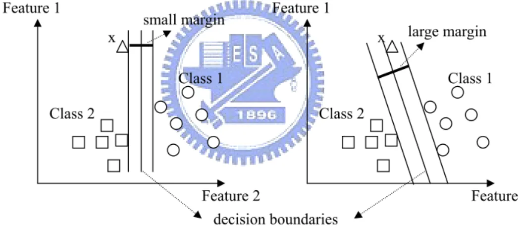
input space into a high dimensional feature space. In this high dimesional feature space, SVM finds a linear hyperplane and use this to make the classification. The corresponding classification using the optimal hyperplane has the two properties: 1) leaving the largest possible part of training samples of the same class on the same side; 2) maximizing the distance of the each class from this hyper plane. If SVM can find the optimal linearly separable hyperplane which minimize the probability of misclassifying the training sam-ples, the unseen test samples will be well classified, too. Figure 2.1 demonstrates the illumination of the learning principle and testing behavior of SVM. In the left diagram with small separating margin, the unknown test sample, x, would be classified to class 2, however, according to the distances between sample x and each class, sample x should belong to class 1. Therefore, the right diagram with large separating margin will provides better test accuracy when coping with the unknown test samples.

Feature 2 Feature 1 Class 1 Class 2 x Feature 2 Feature 1 Class 1 Class 2 x decision boundaries small margin large margin

Figure 2.1. Illumination of the learning principle and testing behavior of SVM.

The SVM is the most popularly used on the microarray data analysis [12, 45, 47, 48, 49]. Because of the characteristic that it is not easily to be overfitting when the number of training samples is small, the SVM performs well on the gene expression data classification problem.

2.1.4 Fuzzy Rule-Base Classifier

There are many machine learning techniques, such as support vector machine (SVM), neural networks (NN), k-nearest neighbor (k-NN), and logistic regression have been used

(26)

in gene expression data classification [12, 13]. However, the learning results of the above-mentioned classifiers cannot be summarized into human-interpretable forms for biologists and biomedical scientists [13]. Fuzzy Rule-Base Classifier not only provides the human-interpretable if-then learning rules but also adopts the “fuzzy” concept to describe the continuous feature value rather than “crisp” one.

The form of a fuzzy if-then rule is:

R : If . . . then Class is . . . .

The most distinguishing property of fuzzy logic is that it deals with fuzzy propositions, that is, propositions which contain fuzzy variables and fuzzy values, for example, “the

gene Xi is up-regulated.” or “the gene Xj is down-regulated.”. However, the truth values

for fuzzy propositions are not binary value , i.e. TRUE/FALSE only, as is the case in propositional boolean logic, but include all the possibilites of certainty grade between two extreme values.

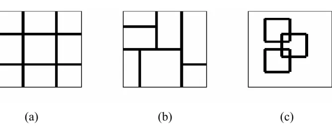
In fuzzy systems, there are three major fuzzy partition methods for the feature space of a membership functions: grid partition, tree partition and scatter partition. In Ho et al. ’s work [37], they are briefly described as follows. Figure 2.2 is the brief illuminations of the three partition method.

Grid Partition

Grid partition is the most commonly used fuzzy partition approach. There may be pn

fuzzy rules in the case of p fuzzy sets on each axis of an n − D feature space using grid partition. A major advantage of grid partition is that fuzzy rules obtained from fixed linguistic fuzzy grids are always linguistically interpretable. However, the grid partition method often results in too many fuzzy rules for human to handle. And the adopted rule filtering strategies often cause the loss of accuracy.

Tree partition

Tree partition results from a series of guillotine cuts. A guillotine cut is made entirely across the subspace to be partitioned, and each of the regions thus produced can then

(27)

be subjected to independent guillotine cutting. Tree partition can significantly relieve the problem of rule explosion and accelerate classification, but its application to high-dimensional problems faces practical problems [50].

Scatter Partition

Scatter partition uses multi-dimensional antecedent fuzzy sets. From the viewpoint of classification performance, scatter partition may be the most effective approach to de-signing high-dimensional fuzzy classifiers [51]. Scatter partition usually generates fewer fuzzy regions than the grid and tree partitions owing to the natural clustering property of training patterns. However, scatter partition of high-dimensional feature spaces is dif-ficult, and thus some learning or automatic evolutionary procedures become necessary [50].

(a) (b)

(c)

Figure 2.2. Illuminations of the three fuzzy partition methods: (a) grid partition; (b) tree partition; (c) scatter partiton.

Each fuzzy partition method forms a corresponding membership functions representing the fuzzy concept mentioned above. Recently, Vinterbo et al. proposed a small and interpretable fuzzy rule-based classifier using a grid partition of feature space for gene expression classification [13]. Because of the continuous and noisy gene expression data of microarray experiments, the fuzzy classifier often makes the classification result more precisely.

(28)

2.2 Models of Genetic Network

The first issue of the inference problem of genetic network is which genetic work model is going to be adopted and to describe the interaction among genes. Based on the nature of the regulation interaction, reverse engineering algorithms for genetic network modeling, in general, can be classified into three categories: by Boolean rules, by stochastic formulas and theory, and by differential equations. In Wu et al. ’s work [52], they summarized the most frequently used models among the four major categories mentioned above: 1) boolean network model, 2) Bayesian network model, 3) linear differential network model, and 4) S-system network model. Following are the brief descriptions about these four models.

2.2.1 Boolean Network Model

Boolean network model is the simplest and the most computationally effective model system that can give some insight into the overall behavior of large genetic networks [53]. In Boolean network models, the interaction between genes can be referred to two situations, true or false (on or off) and the state is determined by a Boolean function of the states of some other genes. These simple models have the advantage that they can be solved with less computing effort. But the drawback is that they can’t quantify interaction intensity between genes and not adequate in analyzing cyclic network structure such as feedback regulatory loops. [54, 55, 56] adopted the Boolean network model to describe the regulation of genetic network.

2.2.2 Bayesian Network Model

Bayesian network model which is able to deal with linear, non-linear, and combinatorial problems is also used to describe genetic networks. Rather than the only two extreme states adopted in Boolean network model, Bayesian network use the stochastic method to model the causality between genes which can quantify degrees of the interactions among networks. There are a set of nodes and a set of edges, which together constitute a directed acyclic graph in a bayesian network. The nodes in the graph represent random variables,

(29)

while the edges indicate the existence of direct causal connections between the linked nodes and the strengths of these connections are expressed in terms of conditional probabilities. But similar to Boolean networks, it suffers from the same dilemma and only applicable to acyclic structures [22, 24]. To cope with the cyclic networks and dynamic modeling the gene regulation, some authors adopted the adapted dynamic Bayesian network [27, 28].

2.2.3 Linear Differential Network Model

The linear differential model is one of the simplest ways to dynamically model the inter-actions between genes. Linear differential models assume that the change of each gene at one time point is determined by a weighted sum of the expressions of all genes at the previous one time point. The mathematical formulism of the linear differential model for a continuous-time system with N genes is described as follows [23]:

dXi(t) dt = N X j=1 wi,j× Xj(t − 1) + bi, i = 1, . . . , N, (2.1)

where Xi(t) is the expression level of the ith gene at time t, N indicates the number of

genes in this genetic network, and bi is a bias term indicating whether gene i is expressed

or not in the absence of regulatory inputs.

The linear differential model is very simple such that it can provide the chance to researchers for finding out the most significant information without taking too complex computational cost. However, there is a major drawback when using the linear differential model: the assumption of linear gene-regulation relationship is unrealistic. To cope with the nonlinear complex systems, such as gene expression networks and metabolic pathways, we need a more general, non-linear, and representative model. [57, 58] applied the linear differential equations to modeling the gene regulation relationship.

2.2.4 S-system Network Model

Another frequently used approach is to use non-linear differential equation models for analysis of gene expression. The most popular model can be referred to the S-system model which has been considered suitable to characterize biochemical network systems and capable to analyze the regulatory system dynamics [29, 30, 31, 32, 33, 34, 35, 26].

(30)

The S-system model is a set of non-linear differential equations as the following form: dXi(t) dt = αi N Y j=1 Xgij j (t − 1) − βi N Y j=1 Xhij j (t − 1) (2.2)

where Xi(t) represents the expression level of gene i at time t and N is the number of

genes in a genetic network. αi and βi are rate constants which indicate the direction of

mass flow and must be positive. gij and hij are kinetic orders which reflect the intensity of

interaction from gene j to i. For inferring an S-system model, it is necessary to estimate

all the 2N (N + 1) S-system parameters (αi, βi, gij, hij) from experimental time-series data

of gene expression.

The S-system models have the ability not only to describe a non-linear gene regulation system but also to cope with the cyclic networks and the dynamic regulation between genes. However, the reverse engineering problem of this general and representative model is a large-scale parameter optimization problem with 2N (N + 1) parameters which is time-consuming and intractable. Genetic algorithm (GA) [36] plays an important role in solving the optimization problem of dynamic modeling of genetic networks using the S-system model [29, 30, 31, 33].

2.3 Genetic Algorithm (GA)

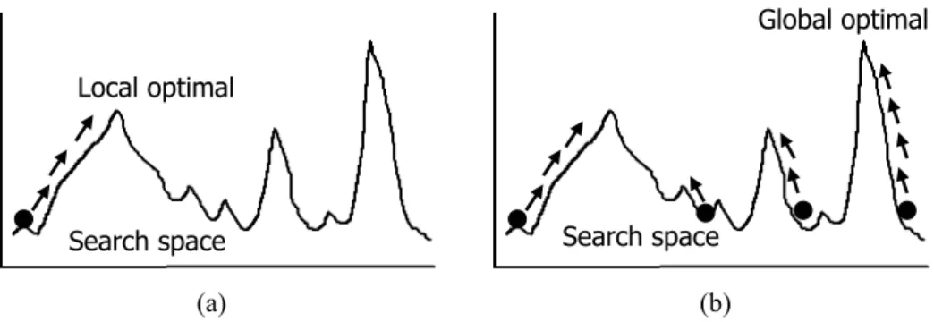
Recently, genetic algorithm (GA) proposed by J. H. Holland in 1970 has become the one of the most popular optimization methods [36]. GA has the advantages that it provides the robust solution quality and that although GA does not need the additional domain knowledge to search the solution space, however, applying appropriate prior knowledge leads to better performance. The main difference between GA and traditional numerical methods is that: 1) GA adopts the coding strategy to transform the candidate solution to “individual chromosome” consisting of a group of parameters; 2) with the population of chromosomes and the specific operators to exchange the information between chromo-somes during searching, GA can efficiently search for the optimal solutions in the search space with high probability to finding out the global optima. Figure 2.3 showes the illumi-nations of the searching models of GA and traditional numerical methods. The qualities

(31)

Search space Local optimal

Global optimal

Search space (a) (b)

Figure 2.3. Illuminations of the searching behaviors between genetic algorithm and tra-ditional numerical method; (a) tratra-ditional numerical method; (b) genetic algorithm.

of the solutions using traditional numerical methods highly depends on the initial given value such that it is easy to fall into local optima.

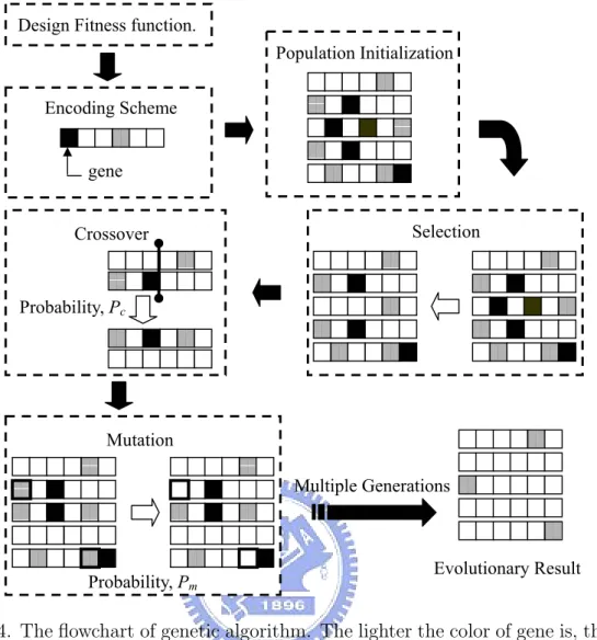
GA consists of three basic operators: 1) Selection: attempting to apply pressure upon the population in a manner similar to that of natural selection found in biological systems; 2) Crossover: allowing solutions to exchange information in a way similar to that used by natural organism undergoing sexual reproduction; 3) Mutation: used to randomly change (flip) the value of single parameter (bit) within the individual chromosome. Figure 2.4 is the flowchart of GA. In this flowchart, the lighter the color of gene is, the better the value of the gene contains. Following are the brief introductions about the major issues in GA: encoding scheme and fitness function, population initialization, selection, crossover, mutation, and termination condition.

2.3.1 Encoding Scheme and Fitness Function

The first stage of building a genetic algorithm is to decide on a genetic representation of a candidate solution to the original problem. This involves defining and arranging each parameter within the individual chromosome and the mapping approach from individual chromosomes and the corresponding candidate solutions to problems being solved.

After deciding on the representation of chromosomes is to design an appropriate fit-ness function. The fitfit-ness functions (or objective functions) are used to quantify each candidate solution mapped from one chromosome, and often, they can be maximized or minimized. Because of the selection operator based on the fitness values a lot, the per-formance of genetic algorithms usually highly depends on the convenience of the adopted

(32)

Design Fitness function. Encoding Scheme gene Population Initialization Selection Crossover Probability, Pc Mutation Probability, Pm Multiple Generations Evolutionary Result

Figure 2.4. The flowchart of genetic algorithm. The lighter the color of gene is, the better the value of the gene contains.

fitness functions.

Following is a simple example for encoding scheme and fitness function design. If we want to maximize the following equation f (x):

f (x) = x2; f or integer x and 0 ≤ x ≤ 4095. (2.3)

We can just use f (x) as the fitness function to be maximized, and adopt the binary representation strategy to encode the value of x such that “110101100100” implies x = 3428 while “010100001100” represents x = 1292.

2.3.2 Population Initialization

One of the characteristics of genetic algorithms is doing parallel search in the solution space with a set of candidate solutions. This set of candidate solutions is called a

(33)

“popu-lation”. To achieve the objective of searching the solution space globally, the chromosomes of populations usually are randomly initialized such that each chromosome will be scat-tered over the solution space uniformly. However, if there are constraints on solutions to the problem being solved, how to guarantee all initial chromosomes feasible is an impor-tant issue to be considered.

2.3.3 Selection

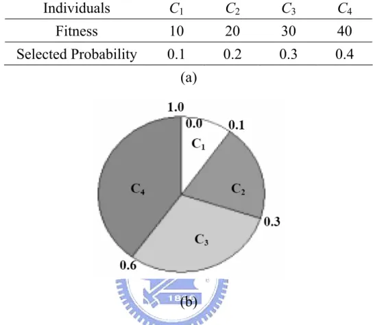
Selection attempts to apply pressure upon the population in a manner similar to that of natural selection found in biological systems. Poorer performing individuals are weeded out and better (fitter) performing ones have a greater chance of promoting the information they contain within the next generation. The typical selection operators can be classified to two categories, parent selection and survivor selection. Both of them are to distinguish among individuals based on their qualities, however parent selection is responsible to allow the fitter individuals to become parents of the next generation, while survivor selection is called after having created the offspring of the selected parents and decide which individual will exist in the next generation. Because of the selection operator, GA can guarantee that after iterated generations, the average quality of the entire population will be improved with a high probability. Following, we will introduce the most common used methods for parent selection: roulette wheel selection and binary tournament selection, and for survivor selection: ranking selection.

Roulette Wheel Selection

With this approach, the probability of selection for one individual is based on the propor-tion of its fitness to the sum of fitness of entire populapropor-tion. Given the fitness value of the

ith individual, fi, and the size of population is Npop, the probability of the ith individual

being selected is:

pi =

fi

PNpop

j=1 fj

. (2.4)

Suppose that there are four individual in the population, and their fitness values and the corresponding selected probabilities are showed in Figure 2.5. For example, in selection, first, randomly generate a real number in [0, 1]. If the real number is in [0, 0.1]

(34)

then child 1, C1 is selected; if the random value is in (0.1, 0.3] then child 2, C2 is selected.

Repeat the steps mentioned above, until the number of individuals in the mating pool is equal to the size of population in the previous generation.

Individuals

C

1

C

2

C

3

C

4

Fitness

10 20 30 40

Selected

Probability 0.1 0.2 0.3 0.4

(a)

(b)

Figure 2.5. An example of roulette wheel selection.

Binary Tournament Selection

The main idea of binary tournament selection is that when doing parent selection, repeat to randomly picking up two individual and place the fitter one to the mating pool, until the number of individuals in the mating pool is equal to the size of population in the previous generation. Compared with roulette wheel selection, in the later period of evolutionary computing, binary tournament selection has a better ability to distinguish the fitter one from two individuals. That is because that in the later period of evolutionary computing, the fitness values of all individual in the population converged such that because of the closed fitness values between individuals, when using roulette wheel selection, it is more difficult to distinguish the better one by two almost the same probabilities. However, even though the fitness values of population have converged, by means of judging which

(35)

one of two has the better fitness, binary tournament selection can still select the better one successfully.

Ranking Selection

Ranking selection is the simplest approach to survivor selection. Rank selection method

replaces the worst Ps× Npop individuals with the best Ps× Npop individuals to form a

new population, where Ps is a selection probability and Npop is the size of population.

Although it is simple, ranking selection have the advantage that it can efficiently speed up the convergence of the entire population and improve the average quality of entire population a lot. [38] adopted ranking selection in their selection operator of GA.

2.3.4 Crossover

The major advantage of genetic algorithm is that with the population of chromosomes (candidate solutions) and the specific operators, crossover, each individual in the pop-ulation can efficiently searching the solution space concurrently. As the name indicate, crossover or recombination allowing two parent individuals to exchange their parameters or information in a way similar to that used by natural organism undergoing sexual

re-production. With a probabilistic parameter, Pc, controlling whether the selected pairs of

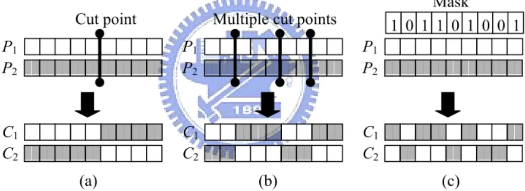
individuals doing crossover or not, we can mate two individuals with different but desir-able features to produce the offspring that combines both of those features. Cooperating with the selection operator, once the better or fitter offspring are generated, they have the higher probability to survive after selection such that the average fitness of population is successfully improved. The most used variations of crossover operator are: one-point crossover, multi-point crossover, and uniform crossover.

One-point Crossover

Before doing one-point crossover, Randomly generate a cut point, then exchange the all parameters of the two parent behind the position of cut point. Figure 2.6(a) shows the behavior of one-point crossover.

(36)

Multi-point Crossover

First, randomly generate multiple cut points. After the positions of multiple cut points are determined, randomly determine whether the parameters of parents between all pairs of successive cut points to be exchange or not. Figure 2.6(b) shows the behavior of multi-point crossover.

Uniform Crossover

Before doing uniform crossover, randomly generate a binary bit string with length being the same as the number of parameters in the individual chromosome. This binary bit string is used as a mask. If a bit value is one, it means that the corresponding parameter should be exchanged, while zero bit implies that the corresponding parameters will not to be exchanged. Figure 2.6(c) shows the behavior of uniform crossover.

P1 P2 C1 C2 Cut point P1 P2 C1 C2

Multiple cut points _{1 0 1 1 0 1}_{0 0 1} P1 P2 C1 C2 Mask (a) (b) (c)

Figure 2.6. Illuminations of (a) one-point crossover, (b) multi-point crossover, and (c) uniform crossover.

2.3.5 Mutation

Mutation operators randomly change (flip) the value of single parameter (bit) within individual chromosome. When doing mutation operation, each parameter or bit in a single individual chromosome is determined whether its value is changed or not based

on a probabilistic parameter Pm. Because of the experiences of medical science, usually,

the mutation brings harmful effects to individuals such that we often set Pm with a

small value. However, the mutation operators still have the significant importance during evolutionary computing. According to the selection and crossover operator, the average

(37)

quality of population will be improved during iterated generations. However, in the last period of evolutionary computing, the fitness values among populations converge and all information contained in the individuals is almost the same. Without producing some new information or parameter values, the entire candidate solutions of population will be trapped into local optima. In this situation, the mutation operator can bring the new information to the entire population such that the population may jump the local optima and find out the global ones.

The mostly used methods of mutation operations are bit flip mutation for binary bit string or randomly generating the perturbing value for each real-valued parameter. The bit flip mutation for binary bit string is that when doing mutation, each bit in the

individual have the probability Pm to flip its value, such as change 1 to 0 or reverse 0

to 1. Figure 2.7 shows the behavior of bit flip mutation. The other commonly used

mutation for real-valued parameters is described below. With a probability Pm, assume

a real-valued parameter x is to be mutated. A perturbation x0 of x is generated by the

Cauchy-Lorentz probability distribution [59]. The mutated value of x is x + x0 or x − x0,

determined randomly.

1 0 0

1 0 1 1 0 1

Mutation point

1 0 0

1 0 0 1 0 1

Figure 2.7. An example of bit flip mutation.

2.3.6 Termination Condition

The termination conditions are the criterions that we terminate the evolutionary search or computing of genetic algorithm. The commonly used termination conditions may be: 1) the average or best fitness values is improved to a default value; 2) The number of generations or fitness evaluation is up to a upper bound set in advance; 3) The best fitness is still not improved after a number of generations; 4) other criterions designed by the users.

(38)

Chapter 3 Intelligent Genetic Algorithm

The used intelligent genetic algorithm (IGA) is a specific variant of the intelligent evolu-tionary algorithm [38] to solve the large-scale parameter optimization problems (LPOP). The main difference between IGA and the traditional GA [36] is an efficient intelligent crossover operation. The intelligent crossover is based on orthogonal experimental design to solve intractable optimization problems comprising lots of design parameters. The following sections describe orthogonal experimental design, factor analysis, intelligent crossover, and the simple intelligent genetic algorithm. The merits of orthogonal exper-imental design and the superiority of intelligent crossover can be further referred to [37] and [38].

3.1 Concept of Orthogonal Experimental Design (OED)

An efficient way to study the effect of several factors simultaneously is to use OED with both orthogonal array (OA) and factor analysis [60, 61, 62]. The factors are the variables (parameters), which affect response variables, and a setting (or a discriminative value) of a factor is regarded as a level of the factor. OED utilizes properties of fractional factorial experiments to efficiently determine the best combination of factor levels to use in design problems.

OA is a fractional factorial array, which assures a balanced comparison of levels of any factor. OA is an array of numbers arranged in rows and columns where each row represents the levels of factors in each combination, and each column represents a specific factor that can be changed from each combination. The term “main effect” designates

(39)

the effect on response variables that one can trace to a design parameter [62]. The array is called orthogonal because all columns can be evaluated independently of one another, and the main effect of one factor does not bother the estimation of the main effect of another factor. Factor analysis using the orthogonal array’s tabulation of experimental results can evaluate the effects of individual factors on the evaluation function, rank the most effective factors, and determine the best level for each factor such that the evaluation function is optimized.

OED can provide near-optimal quality characteristics for a specific objective. Fur-thermore, there is a large saving in the experimental effort. OED specifies the procedure of drawing a representative sample of experiments with the intention of reaching a sound decision [62]. Therefore, OED using OA and factor analysis is regarded as a systematic reasoning method.

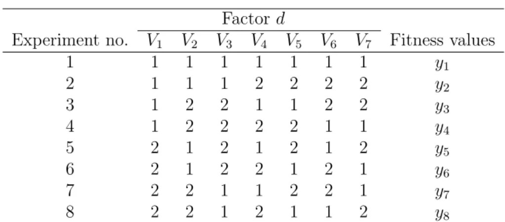
3.2 Orthogonal Array

In this study, the two-level and three-level OAs are used for IGA and OSA [63], respec-tively. The two-level OAs used in IGA are described below. Let there be α factors, with

two levels each. The total number of level combinations is 2α for a complete factorial

experiment. To use an OA of α factors, we obtain an integer M = 2dlog2(α+1)e where the

bracket represents an upper ceiling operation, build an OA LM(2M −1) with M rows and

M − 1 columns, use the first α columns, and ignore the other M − α − 1 columns. OA can reduce the number of level combinations for factor analysis. For instance, Table 3.1

shows an OA L8(27) The number of OA combinations required to analyze all individual

factors is only M = O(α), where α + 1 ≤ M ≤ 2α.

OSA uses three-level OAs where each factor has three levels. The total number of level

combinations for α factors is 3α _{for a complete factorial experiment. To use a three-level}

OA of α factors, we obtain an integer M = 3dlog3(2α+1)e, build an OA L

M(3(M −1)/2) with M

rows and (M − 1)/2 columns, use the first α columns, and ignore the other (M − 1)/2 − α columns. The number of OA combinations required to analyze all individual factors is only M = O(α), where 2α + 1 ≤ M ≤ 6α − 3.

(40)

Table 3.1. An Orthogonal Array of L8(27).

Factor d

Experiment no. V1 V2 V3 V4 V5 V6 V7 Fitness values

1 1 1 1 1 1 1 1 y1 2 1 1 1 2 2 2 2 y2 3 1 2 2 1 1 2 2 y3 4 1 2 2 2 2 1 1 y4 5 2 1 2 1 2 1 2 y5 6 2 1 2 2 1 2 1 y6 7 2 2 1 1 2 2 1 y7 8 2 2 1 2 1 1 2 y8

Algorithm of constructing the two- and three-level OAs can be found in [63]. After proper tabulation of experimental results, the summarized data are analyzed using factor analysis to determine the relative level effects of factors.

3.3 Factor Analysis

Consider the OA LM(2M −1) or LM(3(M −1)/2) is used. Let yt denote a function value of

the combination t, where t = 1, . . . , M . Define the main effect of factor d with level k as

Sdk where d = 1, . . . , α: Sdk = M X t=1 ytWt, (3.1)

where Wt = 1 if the level of factor d of combination t is k; otherwise, Wt = 0. Consider

that the objective function is to be minimized. For the two-level OA, level 1 of factor d makes a better contribution to the objective function than level 2 of factor d does when

Sd1 < Sd2. If Sd1 > Sd2, level 2 is better. If Sd1 = Sd2, levels 1 and 2 have the same

contribution. The main effect reveals the individual effect of a factor. The most effective

factor d has the largest main effect difference M EDd = |Sd1− Sd2|.

For the three-level OA, the level k of factor d makes the best contribution to the

objective function than the other two levels of factor d do when Sdk = min{Sd1, Sd2, Sd3}.

On the contrary, if the objective function is to be maximized, the level k is the best one

when Sdk = max{Sd1, Sd2, Sd3}. The most effective factor has the largest one of main

effect differences M EDd = max{Sd1, Sd2, Sd3} − min{Sd1, Sd2, Sd3}. After the better one

(41)

factors with the better/best levels can be easily derived.

3.4 Intelligent Crossover

All parameters are encoded into a chromosome using binary codes or real values. Like

traditional GAs, two parents P1 and P2 produce two children C1 and C2 in one crossover

operation. Let all encoded parameters be randomly assigned into α groups where each group is treated as a factor. The following steps describe the intelligent crossover opera-tion.

Step 1: Use the first α columns of an OA LM(2M −1).

Step 2: Let levels 1 and 2 of factor d represent the dth groups of parameters coming

from parents P1 and P2, respectively.

Step 3: Evaluate the fitness values yt for experiment t where t = 2, . . . , M . The value

y1 is the fitness value of P1.

Step 4: Compute the main effect Sdk where d = 1, . . . , α and k = 1, 2.

Step 5: Determine the better one of two levels of each factor.

Step 6: The chromosome of C1 is formed using the combination of the better genes

from the derived corresponding parents.

Step 7: The chromosome of C2 is formed similarly as C1, except that the factor with

the smallest main effect difference adopts the other level.

Step 8: The best two individuals among P1, P2, C1, C2, and M − 1 combinations of

OA are used as the final children C1 and C2 for elitist strategy.

One intelligent crossover operation takes M + 1 fitness evaluations, where α + 1 ≤

M ≤ 2α, to explore the search space of 2α combinations.

3.5 The Simple Intelligent Genetic Algorithm

The used IGA is given as follows:

(42)

Step 2: Evaluate fitness values of all individuals. Let Ibestbe the best individual in the

population.

Step 3: Use the simple ranking selection that replaces the worst Ps× Npop individuals

with the best Ps× Npop individuals to form a new population, where Ps is a

selection probability.

Step 4: Randomly select Pc× Npop individuals including Ibest, where Pc is a crossover

probability. Perform intelligent crossover operations for all selected pairs of parents.

Step 5: Apply a conventional bit flip mutation for binary bit string or mutation of randomly generating the perturbing value for each real-valued parameter to

the population using a mutation probability Pm. To prevent the best fitness

value from deteriorating, mutation is not applied to the best individual. Step 6: Termination test: If a pre-specified termination condition is satisfied, stop the

(43)

Chapter 4 Interpretable Gene Expression

Classifier

4.1 The Proposed Interpretable Gene Expression

Clas-sifier (iGEC)

This section proposes an interpretable gene expression classifier (named iGEC) with an accurate and compact fuzzy rule base using a scatter partition of feature space for mi-croarray data analysis. The design of iGEC has three objectives to be simultaneously optimized: maximal classification accuracy, minimal number of rules, and minimal num-ber of used genes. The novel intelligent genetic algorithm introduced in Chapter 3 is used to efficiently solve the design problem with a large number of tuning parameters.

The performance of iGEC is evaluated using eight data sets and high performance of iGEC mainly arises from two aspects. One is to simultaneously optimize all parameters in the design of iGEC where all the elements of the fuzzy classifier design have been moved in parameters of a large parameter optimization problem. The other is to use an efficient optimization algorithm IGA which uses a divide-and-conquer strategy to effectively solve these optimization problems.

4.1.1 Flexible Generic Parameterized Membership Functions

The classifier design of iGEC uses flexible generic parameterized fuzzy regions which can be determined by flexible generic parameterized membership functions (FGPMFs) and a hyperbox-type fuzzy partition of feature space. Each fuzzy region corresponds to a parameterized fuzzy rule. In this study, each value of gene expression is normalized into

運用智慧型基因演算法最佳化微陣列資料分析 - 可語意解讀基因表現量分類器之設計暨基因網路模型之重建

國

立

交

通

大

學

生物資訊研究所

碩

士

論

文

運用智慧型基因演算法最佳化微陣列資料

分析 - 可語意解讀基因表現量分類器之設

計暨基因網路模型之重建

Intelligent Genetic Algorithm for Microarray Data

Analysis – Interpretable Gene Expression Classifier and

Inference of Genetic Network

研 究 生：謝志宏

指導教授：何信瑩 教授

運用智慧型基因演算法最佳化微陣列資料分析 -

可語意解讀基因表現量分類器之設計暨

基因網路模型之重建

Intelligent Genetic Algorithm for Microarray Data Analysis –

Interpretable Gene Expression Classifier

and Inference of Genetic Network

研 究 生：謝志宏 Student：Chih-Hung Hsieh

指導教授：何信瑩 Advisor：Shinn-Ying Ho

國 立 交 通 大 學

生物資訊研究所

碩 士 論 文

運用智慧型基因演算法最佳化微陣列資料分析 - 可語意

解讀基因表現量分類器之設計暨基因網路模型之重建

學生：謝志宏 指導教授：何信瑩

國立交通大學生物資訊研究所

摘 要

Intelligent Genetic Algorithm for Microarray Data Analysis –

Interpretable Gene Expression Classifier and Inference of Genetic Network

Acknowledgements

Contents

List of Figures

List of Tables

Chapter 1

Introduction

1.1

Motivation

1.2

Survey of the Related Works

1.2.1

Gene Expression Classification Problems

1.2.2

Genetic Network Inference Problems

1.3

Sketch of the Thesis

1.3.1

An Interpretable Gene Expression Classifier for Gene

Ex-pression Classification

1.3.2

An Intelligent Two-stage Evolutionary Algorithm for

In-ference of Genetic Network

1.4

Organization

Chapter 2

Background

2.1

Classifiers for Gene Expression Classification

2.1.1

Neural Networks (NN)

2.1.2

k-nearest-neighbor Rule (k-NN)

2.1.3

Support Vector Machine (SVM)

2.1.4

Fuzzy Rule-Base Classifier

(a) (b)

(c)

2.2

Models of Genetic Network

2.2.1

Boolean Network Model

研究生：謝志宏

指導教授：何信瑩教授

研究生：謝志宏 Student：Chih-Hung Hsieh

國立交通大學

碩士論文

學生：謝志宏指導教授：何信瑩

摘要