行政院國家科學委員會專題研究計畫 期中進度報告
子計畫三:父母死亡、職業傷殘對小孩教育發展的影響
(I)(1/2)
計畫類別: 整合型計畫 計畫編號: NSC93-2621-Z-002-013- 執行期間: 93 年 08 月 01 日至 94 年 10 月 31 日 執行單位: 國立臺灣大學經濟學系暨研究所 計畫主持人: 劉錦添 報告類型: 完整報告 處理方式: 本計畫可公開查詢中 華 民 國 94 年 5 月 18 日
Parental Sick, Loss and Children Education Achievement in
Taiwan
(Mid-term Report)
Jin-Tan Liu*, Shin-Yi Chou** and Hung-ju Chen***
May 2005
Abstract
Keywords: Parental Loss, Education Achievement, Taiwan JEL Classification:
________________________
* Department of Economics, National University and NBER. ** Department of Economics, Lehigh University and NBER. ***Department of Economics, National Taiwan University.
Corresponding author: Jin-Tan Liu, Department of Economics, National Taiwan University, 21 Hsu-Chow Road, Taipei 100, Taiwan. Tel: (886-2)2351-9641 ext. 520, fax: (886-2)2321-5704, 2351-1826; E-mail: [email protected]
1. INTRODUCTION
Besides schools, parental involvement would be the most important determinant to the human capital accumulation of their children. Parents not only provide financial supports for their children, but also educate their children. A loss of a parent might be the most drastic shock to a child. It reduces the educational and health investments for the children because of the lower financial resources. Furthermore, the emotional status would also affect the human capital accumulation of the next generation
There has already been quite a substantial body of literature studying the accumulation of human capital through intergenerational altruism (Uzawa (1965), Loury (1981), Becker and Tomes (1979), Becker and Tomes (1986) and Lucas (1988)). Theses works analyze the role of parental income/human capital in the human capital accumulation for their children. Becker et. al. (1990) showed that there is a quantity-quality trade-off between the fertility decision and educational investment per child as parental human capital increases. Similar results can be also found in the study of de la Croix and Doepke (2003). Bell et al. (2003) developed a dynamic model to study the impact of the parental loss on economic growth. The empirical work by Gertler et. al. (2002) and Evans and Miguel (2004) found that the loss of a parent will reduce children’ school participation.
We construct an overlapping generations (OLG) model within which agents differ in both their emotional status and in the human capital and status possessed by their parents, and study the impacts of the parental loss on the human capital accumulation of the next generation. Despite human capital being widely regarded as an extremely important engine of economic growth, rather surprisingly, few studies within the literature have attempted to examine the link between health condition and
human capital accumulation. It is well-known that a student with better health condition can learn better than students with poor health condition. The health condition can be characterized by the physical status and emotional status. We first consider the physical status of children. Assuming that increasing health investment can increase life expectancy, Leung and Wang (2002) constructed a theoretical model and demonstrated that there is positive relationship between health investment and economic growth. In this paper, we assume that parents not only make decisions on educational investment, but also on the health investment for their children. An increase of the health investment will improve children’s health condition and hence, it will increase schooling hours for children. The results demonstrate that both educational spending and health investment are positively correlated with parental human capital/income. Therefore, the death of a parent will lower the educational and health investment for the children.
We then extend the model by considering the emotional status of children by incorporating the shock of parental loss into the accumulation function of human capital and analyze effects of an early parental loss and a late parental loss on the college entrance examination. Our results illustrates that if an early loss of a parent does not cause a large reduction in financial resources for children, then an early parental loss will have smaller impact on children’s performance of the entrance examination then a late parental loss.
2. The Theoretical Model
We consider an infinite-horizon, discrete-time overlapping generations model where agents live for two periods. Each period corresponds to youth and old age (adulthood). We assume that the initial cohorts were born as adults. Every adult gives birth to a young person and a family is composed by an adult and his/her child. We refer to
young agents as children and to adults as parents. There is no population growth and we normalize population size to one.
Each agent is endowed with one unit of time in each period. Moreover, young agents can be differentiated by the parental human capital (h as well as the t) statuses of their parents and themselves. Young agents spend n units of time in t school. The rest of time (1−nt) is lost due to illness. The accumulation function of human capital depends on the educational investments, schooling time, parental human capital and statuses of children and parents. Hence, it is represented as
ht+1 = Atqαt nθt (φtht)δ, α,θ,δ∈(0,1), (1) where q is the educational investment. The parameter t At >0 captures the characteristics of children such as the innate ability and emotional status and we refer this as the status of children. The other parameter
φ
t describes the status of parents. In this paper, we focus the impacts of parental loss; hence, we useφ
t to represent the reduction of the contribution from parental human capital to children’s human capital accumulation.1 Equation (1) indicates that children’s human capital is an increasing function of the educational investment, schooling time and parental human capital. The parametersα
, θ and δ are elasticities of children’s human capital to the educational investment, schooling time and parental human capital. We assume that the human capital accumulation function exhibits decreasing returns to scale; that is,1 < + +θ δ
α .
The hours that a child spends in school depends on his/her health condition. We assume that parents can improve their children’s heath condition by spending more on health investment, I . The impact of health investment on schooling hours can be t
represented by
1 As it will become clear later, t
φ
also can be interpreted as the reduction of family income due to the parental loss.)γ 1 ( ) ( 1 t t t t t I I n I n n + = = , )
γ
∈(0,1 . (2) We assume that 0<n1 ≤1 to reflect the fact that maximal schooling time cannot exceed the time endowment. The properties of nt(It) are as follows:nt'(It)>0, nt ''(It)<0, =∞
→ '( )
lim
0 t t
It n I and Ilimt→∞nt'(It)=0. Substituting equation (2) into equation (1) shows that children’s human capital positively depends on the health investment.
Parents spend all their time for work. Because physical capital is not included in the model, we assume that in period t , adults’ income equals their human capital, h . t
Given the wage income, parents need to decide how much to consume, how much to spend on children’s education and health and how much bequests (b ) to leave for t
their children. Following Becker and Tomes (1986), we assume that parents can borrow from their children’s income to finance their expenditures (if bt <0) and children need to pay for their parent’s debt when they become adults. Agents have the same utility function over their lifecycle. We assume that parents are altruistic and care about their children’s wealth (ht+1 +Rtbt) and their won consumption. The utility function is represented by
ln(ct)+
β
ln(ht+1+Rtbt), (3) where c represents the consumption of adults born at time t t−1, R represents the treal interest rate and
β
is the discount factor. In this paper, we consider a small, open economy and hence, the real interest rate is assumed to be constant (Rt =R,t
∀ ).
The budget constraint for adults is
ct +qt +It +bt =wt, (4) where wt =
φ
tht +Rbt−1 is the wealth for the family in period t .optimal choices of educational spending, health investment and bequest are t t t t t h Rb q h c ( ) 1 1 1 + = + +
αβ
, (5) t t t t t t t h Rb n I n h c ( ) ) ( ' 1 1 1 + = + +βθ
, (6) t t t h Rb R c = +1+ 1 β . (7) Using equations (5) and (7), we can gett = ht+1 R
q α . (8) Using equations (5) and (6), we can obtain
) ( ' ) ( ) ( t t t t t t t I n I n I q q
θ
α
= = . (9) Combining equations (1), (2), (8) and (9), we then deriveAtItα+γθ− + It α−γθ− φtht δ 1−α = B 1 1 1 ] ) ( ) 1 ( [ , (10) where α θ α α
α
θγ
+ − = 1 1 1 ) ( 1 R n B .We first consider the situation when there are no changes of children’s and parents’ statuses and study the impacts of parental human capital on children’s human capital accumulation.
Proposition 1. Given the same statuses of children and parents, the health investment and schooling time are positively correlated with parental human capital.
Proof.
Taking the total derivative of equation (10), then we can get the following relationship between I and t h for constant t A and t
φ
t:0 )] 1 ( 2 ) 1 [( ) 1 ( > − + − − + =
α
γθ
α
δ
t t t t t t I h I I dh dI . (11) To examine the impact of parental human capital on schooling time, note that from equation (2), we can derive that nt'(It)>0. Hence,= '( ) >0 t t t t t t dh dI I n dh dn . (12) Equations (11) and (12) states that the health investment and schooling time will increase as parental human capital increases.
Q.E.D.
Proposition 2. Given the same statuses of children and parents, parents with higher human capital will invest more on their children’s education than parents with lower human capital.
Proof.
First note that from equation (9), we know that
0 )] ( ' [ ) ( '' ) ( }] ( ' [ ) ( ' 2 2 > − = t t t t t t I n I n I n I n I q
θ
α
. Hence, = '( ) >0 t t t t t t dh dI I q dh dq . (13) Q.E.D.Proposition 1 demonstrates that with the same statuses of children and parents, parents with higher human capital will spend more on their children’s health and therefore, their children will spend more time in school. Another important determinant of the human capital accumulation for children is the educational investment and Proposition 2 demonstrates that educational investment is also an increasing function of parental human capital. Because educational investment and schooling time can be represented as functions of parental human capital, then the human capital function for children can be represented as
) , , ( ) ), ( , , ( 1 1 1 t t t t t t t t t t t t h A q n I h h A h h+ = +
φ
= +φ
. (14)Equation (14) shows that the human capital accumulation for children depends on the status of their parents and themselves as well as parental human capital. The
following proposition presents the linkage between parental and children’s human capital.
Proposition 3. Given the same statuses of children and parents, children belonging to high-income parents (or equivalently, parents with higher human capital) will accumulate higher human capital then children belonging to low-income parents.
Proof.
From equation (14), we can get t t t t t t t t t t t t h h dh dn n h dh dq q h dh dh ∂ ∂ + ∂ ∂ + ∂ ∂ = + + + +1 1 1 1 . (15) From the human capital accumulation function (equation (2)), we know that
1 >0 ∂ ∂ + t t q h , 1 >0 ∂ ∂ + t t n h and 1 >0 ∂ ∂ + t t h h . Furthermore, propositions 1 and 2 exhibit that
>0 t t dh dq and >0 t t dh dn . Hence, 1 >0 ∂ ∂ + t t h h
. That is, there is a positive linkage between the children’s and their parents’ human capital.
Q.E.D.
2.1 Parental Loss
In this section, we examine the impacts of parental loss and use the status of parents (
φ
t) to indicate the deaths of parents or not. To simplify our analysis, we assume that when the death of a parent occurs, the family financial resources will be reduced by a constant fraction (1−φ
1). We then normalizeφ
t =1 for the case when there is no parental loss andφ
t =φ
1 <1 if there is a parental loss due to the decrease of supports from parents. As pointed out by Gertler et al. (2002), children may get some formal insurance invested by their parents or informal insurance from relatives, neighbors orthe society when losing their parents, we assume that
φ
1 is greater than zero. From equation (10), we can derive that{ ( )} ) ( 1 t t t t t t t t t h h d A dA I I dI
φ
φ
δ
+ Γ = , (16) where 0 ) 1 ( ) 1 ( 2 1 ) ( > + − + − − = Γ t t t I I Iα
γθ
α
.Proposition 4. Given the same status of children, the losses of parents will affect the health investment for children with low-income parents more than children with high-income parents.
Proof.
From equation (16), we can get the percentage change of health investment when there is a parent loss
0 ) ( ) /( ) ( / > Γ = t t t t t t t I h h d I dI
δ
φ
φ
. (17)Equation (17) shows that the loss of a parent will cause a reduction on health investment. Note that ( ) (1
φ
1)φ
φ
=− − t t t t h h dwhen the death of a parent occurs. Hence, when a parental loss happens, the percentage change of health investment will be 0 ) ( ) 1 ( 1 < Γ − − = t t t I I dI
δ
φ
.Let )Λ(It represent the absolute value of dI /t It. We then get
0 ] ) 1 ( 2 1 [ ) 1 )( 1 ( ) ( ' 1 2 < − + − − − − − − = Λ t t I I
α
γθ
α
γθ
α
φ
δ
. (18) Equation (18) illustrates that the percentage reduction of children’s health investment due to the parental loss is negatively correlated with the health investment without parental losses. Furthermore, Proposition 1 has shown that high-income parents will invest more on their children’s health. Therefore, the losses of parents will affect the health investment for children with rich parents less than children with low-income parents.Proposition 5. Given the same status of children, the loss of a parent will have larger impacts on the human capital accumulation of the child belonging to low-income parents.
Proof.
From equation (2), we know the linkage between the percentage change of schooling time and the percentage of health investment:
t t t t t I dI I n dn ) 1 ( 1 + =
γ
. (19)Also, equations (8) and (1) imply that
{ ( )} 1 1 t t t t t t t t t t h h d n dn A dA q dq
φ
φ
δ
θ
α
+ + − = , (20) t t t t t t t t t t t t h h d n dn q dq A dA h dhφ
φ
δ
θ
α
( ) 1 1 = + + + + + . (21)Combining equations (19), (20) and (21), we then get
( )} ) 1 ( { 1 1 1 1 t t t t t t t t t t t h h d I dI I A dA h dh
φ
φ
δ
γ
θ
α
+ + + − = + + . (22)Using equation (17) to substitute t t
I dI
in equation (22), we then obtain
}{ ( )} ) ( ) 1 ( 1 { 1 1 1 1 t t t t t t t t t t h h d A dA I I h dh
φ
φ
δ
γ
θ
α
+ + Γ + − = + + . (23)With the same status of children, a parental loss will cause the percentage change of children’s human capital as
}(1 ) 0 ) ( ) 1 ( 1 { 1 1 1 1 − < Γ + + − − = + +
φ
γ
θ
α
δ
t t t t I I h dh . (24) Equation (24) indicates that a loss of a parent will lower the child’s accumulation of human capital. Let Ω(It) represent the absolute value of1 1 + + t t h dh in equation (24), then 0 ] ) 1 ( 2 1 [ ) 1 ( 2 ) ( ' 1 2 < − + − − − − = Ω t t I I
α
γθ
α
γ
φ
δθ
. (25) Since high-income parents will have higher I , the loss of a parent will have smaller timpacts on the human capital accumulation of a child belonging to high-income parents.
Q.E.D.
2.2 Long-run versus Short-run Effects
In the previous section, we do not consider the status of children when the parental loss happens. If we consider the emotional status for children when there is a parental death, then its impacts would be even larger. Furthermore, in this section, we want to compare the impacts of an early parental loss and a late parental loss on children’s performance of the college entrance examination. Most children in Taiwan take the college entrance examination at age 18.
We refer it as the case of an early parental loss if children lose their parents before age 6 and as the case of a late parental loss if children lose their parents around age 15. To lose a parent at the early age would induce a larger reduction on both the health and educational investments for the child than losing a parent at later age. We use
φ
2 andφ
3 to denote the reduction of the financial resource when there is an early parental loss and a late parental loss, respectively. Hence, 1>φ
3 >φ
2. A lateparental loss which is close to the timing of the college entrance examination will cause severe emotional disturbances for the children. We use A1, A2 and A to 3
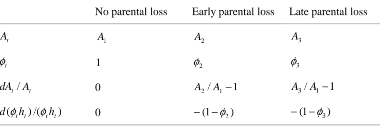
indicate the emotional status of a child when there is no parental loss, an early parental loss and a late parental loss, respectively. Hence, A1 > A2 > A3. Table 1
summarizes the impacts of early and late parental losses comparing with the case without parental losses. The effects of an early and late parental loss are demonstrated in Proposition 6.
Table 1. Impacts of an early parental loss and a late parental loss
No parental loss Early parental loss Late parental loss t A A1 A2 A 3 t
φ
1φ
2φ
3 t t A dA / 0 A2/A1 −1 A3/A1−1 ) /( ) ( tht tht dφ
φ
0 −(1−φ
2) −(1−φ
3)Proposition 6. Given the same parental human capital, if the difference between
φ
2 andφ
3 is small enough or if the difference between A2 and A is large enough, an 3early parental loss will be cause a smaller percentage reduction of the human capital accumulation of a child than a late parental loss.
Proof.
Equation (23) indicates that with an early loss of a parent, the percentage change of
1 + t h is }{(1 ) (1 )} ) ( ) 1 ( 1 { 1 1 2 1 2 1 1
δ
φ
γ
θ
α
+ + Γ − + − − − = + A A I I h dh t t e t t . With a late loss of a parent, the percentage change of ht+1 is}{(1 ) (1 )} ) ( ) 1 ( 1 { 1 1 3 1 3 1 1
δ
φ
γ
θ
α
+ + Γ − + − − − = + + A A I I h dh t t l t t . Hence, l t t e t t h dh h dh 1 1 1 1 + + + + < if 1 3 2 2 3 ) ( A A Aδ
φ
φ
− < − . Q.E.D.Proposition 6 illustrates that if the reduction of the financial resources due to an early parental loss is not very large (
φ
2 is not very low) or if a late parental loss induces a drastic impact on the child’s emotion (A is very low), then an early 3parental loss will cause less severe impacts on the child’s performance in the examination than a late parental loss.
3. Empirical
Model
3.1 Ordinary Least Squares
:
3.2 Propensity Scoring Matching:
B. Propensity Score Matching Method
Matching methods, pairing treatment and control units that have similar observable attributes, eliminate the potential bias due to observable differences. To reduce the difficulties of matching based on high dimensionality of the observable characteristics, Rosenbaum and Rubin (1983) show that matching on the basis of multidimensional vector of pre-treatment characteristics X is equivalent to matching based on the propensity score p(X). The propensity score gives the conditional probability of receiving a treatment given pre-treatment characteristics X, i.e.,
) | 1 Pr( ) (X D X
p ≡ = . Thus, conditional on p(X), the assignment to the treatment and
control groups is random (assumption of ignorability) and matching methods will yield an unbiased estimate of the treatment effect on the treated.
We first estimate the propensity scores from a logit model that a parental loss as a function of the pre-treatment characteristics (Imbens 2000). The results in the first-stage are reported in Appendix A. These models are then used to predict the propensity (probability) of being a parental loss. Then for each family in the treatment group, we match a parental loss family (control group) using the nearest neighborhood matching and kernel matching methods.
Nearest neighborhood matching requires each treated unit i∈T to be matched to the nearest controlled unit, even if a controlled unit is matched more than once
(Becker and Ichino 2002). That is, || || min ) ( i j j p p i C = −
where C(i) denotes a singleton set of control unit matched to the treated unit i.2 Then the matching estimator (τ) can be written as follows:
∑
∑
∈ ∈ − = T i j C i C j ij T i T Y w Y N () 1τ
, = ∈ = otherwise. , 0 ) ( if , 1 ij C i ij w i C j N wwhere N denotes the number of observations in the treatment group, and T C i
N
denotes the number of controls matched with observation i∈T . In practice, C i N is likely to be one. T i Y and C j Y
are the observed outcomes of the treated and control units, respectively. The advantage of using a single controlled unit for each treatment unit is to ensure the smallest propensity-score distance between the treatment and controlled units; that is, we will be comparing very similar control and treatment units. However, the precision of the estimates will be improved if more controlled units are matched, but at the cost of increased bias (i.e. matched controlled units could be very different from the treatment unit) (Dehejia and Wahba, 2002).
Since results could be very sensitive to the matching methods, kernel matching method is also employed to reassure the robustness of our results. The kernel matching estimator is given by
2
In practice, multiple nearest neighbors should be very rare, especially when the propensity scores are estimated based on a large array of continuous variables.
∑
∑
∑
∈ ∈ ∈ − − − = T i C k n i k C j n i j C j T i T k h p p G h p p G Y Y N ) ( ) ( 1τ
where G(.) is a kernel function and hn is a bandwidth parameter. In kernel matching, all treated as well as all controls units, will be used.
REFERENCES
Becker, G.S., K.M. Murphy and R. Tamura (1990), “Human Capital, Fertility, and Economic
Growth, ” Journal of Political Economy 98: 12-37.
Becker, G.S. and N. Tomes (1979), “An Equilibrium Theory of the Distribution of Income
and Intergenerational Completion, ” Journal of Political Economy 87: 1153-8.
Becker, G.S. and N. Tomes (1986), “Human Capital and the Rise and Fall of Families,”
Journal of Labor Economics 4: S1-39.
Bell, C., Devarajan, S. and Gersbach, H. (2003), “The Long-run Economic Costs of AIDS:
Theory and an Application to South Africa,” Mimeo. Sid-Asien Institut, University of
Heidelberg.
de la Croix, D. and M. Doepke (2003), “Inequality and Growth: Why Differential Fertility
Matters,” American Economic Review 93: 1091-1113.
Dehejia, Rajeev H.. and Sadek Wahba (2002), “Propensity Score Matching Methods for
Non-Experimental Causal Studies,” Review of Economics and Statistics, 84: 151-161.
Downey, Douglas B. (1994), “The School Performance of Children from Single-Mother and
Single-Father Families,” Journal of Family Issues, 5: 129-174.
Evans, D. and Miguel, E. (2004), ‘Orphans and Schooling in Africa: A Longitudinal
Analysis’. Mimeo. Harvard University.
Gertler, P., D. Levine and M. Ames (2002), “Schooling and Parental Death,” Review of
Economics Statistics, 86: 211-225.
Kehoe, T. and D. Levine (1993), “Debt-Constrained Asset Markets,” Review of Economic
Studies’, 60: 865- 888.
Leung, C.M. and Y. Wang (2002), ‘Endogenous Health Care, Life Expectancy, and Economic
Growth’. Mimeo. Chinese University of Hong Kong.
Lochner, L. and A. Monge-Naranjo (2002), ‘Human Capital Formation with Endogenous
Loury, G.C. (1981), “Intergenerational Transfers and the Distribution of Earnings,”
Econometrica 49: 843-867.
Lucas, R.E., Jr. (1988), “On the Mechanics of Economic Development,” Journal of Monetary
Economics 22: 3-42.
Uzawa, H. (1965), “Optimum Technical Change in an Aggregative Model of Economic
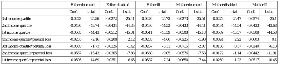
Table 1: Education Achievement
Dependent Variable: Attending University=1
OLS Regression
Father deceased Father disabled Father ill Mother deceased Mother disabled Mother ill
Coef. t-stat Coef. t-stat Coef. t-stat Coef. t-stat Coef. t-stat Coef. t-stat
3rd income quartile -0.0273 -25.56 -0.0272 -25.41 -0.0276 -25.73 -0.0273 -25.51 -0.0272 -25.47 -0.0274 -25.1
2nd income quartile -0.0430 -43.74 -0.0434 -44.35 -0.0436 -44.52 -0.0433 -44.41 -0.0434 -44.54 -0.0433 -43.68
1st income quartile -0.0505 -44.43 -0.0512 -45.31 -0.0511 -45.39 -0.0508 -45.18 -0.0509 -45.37 -0.0508 -44.58
4th income quartile*parental loss -0.0255 -2.16 0.0208 2.12 -0.0283 -4.66 -0.0225 -1.93 0.0324 2.22 0.0003 0.1
3rd income quartile*parental loss -0.0359 -1.73 -0.0226 -1.42 -0.0267 -3.31 -0.0715 -2.97 0.0130 0.37 -0.0240 -6.13
2nd income quartile*parental loss -0.0567 -15.43 -0.0365 -7.83 -0.0560 -9.05 -0.0576 -7.53 -0.0172 -1.14 -0.0442 -11.91
1st income quartile*parental loss -0.0595 -14.69 -0.0351 -6.65 -0.0587 -7.24 -0.0650 -7.44 -0.0250 -1.23 -0.0517 -10.45
Propensity Score Matching Method
Father deceased Father disabled Father ill Mother deceased Mother disabled Mother ill
Coef. t-stat Coef. t-stat Coef. t-stat Coef. t-stat Coef. t-stat Coef. t-stat
3rd income quartile -0.022 -17.627 -0.022 -17.6 -0.022 -17.772 -0.022 -17.634 -0.022 -17.614 -0.022 -17.474
2nd income quartile -0.039 -34.481 -0.039 -35.074 -0.039 -35.054 -0.039 -35.175 -0.039 -34.489
1st income quartile -0.046 -36.208 -0.047 -36.822 -0.047 -36.733 -0.047 -36.886 -0.047 -36.19
4th income quartile*parental loss -0.026 -1.913 0.019 1.49 -0.024 -3.855 -0.025 -1.829 0.029 1.44 0 0.038
3rd income quartile*parental loss -0.035 -1.572 -0.021 -1.246 -0.02 -2.567 -0.067 -3.441 0.016 0.365 -0.02 -5.037
2nd income quartile*parental loss -0.053 -16.383 -0.037 -7.985 -0.05 -9.564 -0.053 -8.02 -0.018 -1.033 -0.042 -11.713
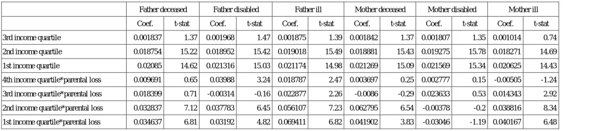
Table 2: Health Outcome
Dependent Variable: Number of hospital visits (96/8-98/5)
OLS Regression
Father deceased Father disabled Father ill Mother deceased Mother disabled Mother ill
Coef. t-stat Coef. t-stat Coef. t-stat Coef. t-stat Coef. t-stat Coef. t-stat
3rd income quartile 0.001837 1.37 0.001968 1.47 0.001875 1.39 0.001842 1.37 0.001807 1.35 0.001014 0.74
2nd income quartile 0.018754 15.22 0.018952 15.42 0.019018 15.49 0.018881 15.43 0.019275 15.78 0.018271 14.69
1st income quartile 0.02085 14.62 0.021316 15.03 0.021174 14.98 0.021269 15.09 0.021569 15.34 0.020625 14.43
4th income quartile*parental loss 0.009691 0.65 0.03988 3.24 0.018787 2.47 0.003697 0.25 0.002777 0.15 -0.00505 -1.24
3rd income quartile*parental loss 0.018399 0.71 -0.00314 -0.16 0.022877 2.26 -0.0086 -0.29 0.023633 0.53 0.014343 2.92
2nd income quartile*parental loss 0.032837 7.12 0.037783 6.45 0.056107 7.23 0.062795 6.54 -0.00378 -0.2 0.038816 8.34
1st income quartile*parental loss 0.034637 6.81 0.03192 4.82 0.069411 6.82 0.041902 3.83 -0.03046 -1.19 0.040167 6.48
Propensity Score Matching Method
Father deceased Father disabled Father ill Mother deceased Mother disabled Mother ill
Coef. t-stat Coef. t-stat Coef. t-stat Coef. t-stat Coef. t-stat Coef. t-stat
3rd income quartile 0.003 2.225 0.003 2.403 0.003 2.266 0.003 2.182 0.003 2.175 0.002 1.485
2nd income quartile 0.02 15.131 0.02 15.472 0.02 15.502 0.02 15.35 0.02 15.672 0.019 14.614
1st income quartile 0.022 14.465 0.022 14.876 0.022 14.739 0.022 14.817
4th income quartile*parental loss 0.009 0.722 0.04 2.403 0.019 2.36 0.005 0.408 0.002 0.116 -0.004 -1.319
3rd income quartile*parental loss 0.02 0.88 -0.004 -0.181 0.025 2.293 -0.006 -0.23 0.025 0.644 0.016 2.97
2nd income quartile*parental loss 0.035 6.782 0.039 4.906 0.058 5.483 0.064 5.158 -0.001 -0.099 0.04 6.45
1st income quartile*parental loss 0.037 5.658 0.034 4.518 0.071 5.486 0.043 3.595 -0.031 -1.797 0.042 5.468