使用蛋白質表面三度空間的交互作用原子機率分布以預測蛋白質-蛋白質交互作用區域

國 立 交 通 大 學

生物資訊及系統生物研究所

博

士 論 文

使用蛋白質表面三度空間的交互作用原子機

率分布以預測蛋白質-蛋白質交互作用區域

PROTEIN-PROTEIN INTERACTION SITE

PREDICTIONS WITH THREE-DIMENSIONAL

PROBABILITY DISTRIBUTIONS OF

INTERACTING ATOMS ON PROTEIN

SURFACES

研 究 生：陳鯨太

指導教授：許聞廉 教授

何信瑩 教授

使用蛋白質表面三度空間的交互作用原子機率分布

以預測蛋白質-蛋白質交互作用區域

Protein-Protein Interaction Site Predictions with

Three-Dimensional Probability Distributions of Interacting

Atoms on Protein Surfaces

研 究 生：陳 鯨 太 Student : Ching-Tai Chen 指導教授：許 聞 廉 博士 Advisors: Dr. Wen-Lian Hsu

何 信 瑩 博士 Advisors: Dr. Shinn-Ying Ho

國 立 交 通 大 學

生 物 資 訊 及 系 統 生 物 研 究 所

博 士 論 文

A Dissertation

Submitted to Institute of Bioinformatics and Systems Biology College of Biological Science and Technology

National Chiao-Tung University in Partial Fulfillment of the Requirements

for the Degree of Ph.D. in

Bioinformatics July 2012

Hsinchu, Taiwan, Republic of China

使用蛋白質表面三度空間的交互作用原子機率分布以預測蛋

白質-蛋白質交互作用區域

研究生：陳鯨太

指導教授：許聞廉 博士 與 何信瑩 博士

國立交通大學生物資訊與系統生物研究所

摘

要

蛋白質-蛋白質交互作用是很多生物程序的關鍵。用來預測蛋白質-蛋白質交互作用 區域的計算方法論是相當重要的工具，能夠提供對於蛋白質功能的深入瞭解、以 及發展針對於蛋白質-蛋白質交互區域的治療方法。蛋白質-蛋白質交互區域的一項 共通特徵是兩個蛋白質交互作用的表面有互補性，類似蛋白質內部的堆積密度及 氨基酸組成的物理化學特性。在此研究中，我們在蛋白質表面建構非共價鍵交互 作用原子的三度空間機率密度地圖以模擬物理化學性質的互補性。交互作用原子 的機率是從蛋白質內部統計而來，機器學習方法則被應用於學習蛋白質-蛋白質交 互作用區域上機率密度地圖的特徵模式。經過訓練的預測機使用一組學習案例(包 含 432 條蛋白質)作為交互驗證之用，並且使用獨立的資料組(包含 142 條蛋白質) 作測試。獨立測試結果中，以氨基酸為單位的馬修斯相關係數為 0.423，正確率、 精準度、靈敏度、特異性分別為 0.753、0.519、0.677 以及 0.779。量測的結果顯示 我們最佳化的機器學習模型是現今最準確的預測機之一。當蛋白質-蛋白質交互作 用區域變大以及當此區域的氨基酸組成擁有更多疏水性時，預測準確率會提高; 而

蛋白質交互作用區域的核心較有可能被給予高預測信心值。我們的結果表示蛋白 質表面的物理化學互補性質是決定蛋白質-蛋白質交互作用的重要因素，而使用蛋 白質內部擷取的非共價鍵交互作用資料所產生出的物理化學互補性特徵，能夠準 確地預測出相當大比例的蛋白質-蛋白質交互作用區域。

Protein-Protein Interaction Site Predictions with

Three-Dimensional Probability Distributions of Interacting Atoms

on Protein Surface

Student: Ching-Tai Chen

Advisors: Dr. Wen-Lian Hsu and Dr. Shinn-Ying Ho

Institute of Bioinformatics and Systems Biology National Chiao-Tung University

Abstract

Protein-protein interactions are key to many biological processes. Computational methodologies devised to predict protein-protein interaction (PPI) sites on protein surfaces are important tools in providing insights into the biological functions of proteins and in developing therapeutics targeting the protein-protein interaction sites. One of the general features of PPI sites is that the core regions from the two interacting protein surfaces are complementary to each other, similar to the interior of proteins in packing density and in the physicochemical nature of the amino acid composition. In this work, we simulated the physicochemical complementarities by constructing three-dimensional probability density maps of non-covalent interacting atoms on the protein surfaces. The interacting probabilities were derived from the interior of known structures. Machine learning algorithms were applied to learn the characteristic patterns of the probability density maps specific to the PPI sites. The trained predictors for PPI sites were

cross-validated with the training cases (consisting of 432 proteins) and were tested on an independent dataset (consisting of 142 proteins). The residue-based Matthews correlation coefficient for the independent test set was 0.423; the accuracy, precision, sensitivity, specificity were 0.753, 0.519, 0.677, and 0.779 respectively. The benchmark results indicate that the optimized machine learning models are among the best predictors in identifying PPI sites on protein surfaces. In particular, the PPI site prediction accuracy increases with increasing size of the PPI site and with increasing hydrophobicity in amino acid composition of the PPI interface; the core interface regions are more likely to be recognized with high prediction confidence. The results indicate that the physicochemical complementarity patterns on protein surfaces are important determinants in PPIs, and a substantial portion of the PPI sites can be predicted correctly with the physicochemical complementarity features based on the non-covalent interaction data derived from protein interiors.

ACKNOWLEDGEMENT

這篇博士論文的完成，首先要感謝我的指導教授許聞廉、以及帶領研究的楊安 綏老師，兩位老師僅管指導學生的方式不盡相同，但對於學術的熱誠以及嚴謹的 研究態度卻一致，我在接受兩位老師指導的過程中獲益良多，此外這些年的相處 讓我有幸見識到頂尖學者應該具備的特質，不論是學術或待人處世上，都是我學 習的典範。宋定懿老師在我擔任研究助理以及博士班初期也曾經指導過我，她在 論文的論述及英文寫作方面提供我相當大的幫助，此外我還要感謝論文口試委員 黃鎮剛老師、何信瑩老師、以及楊進木老師，他們在百忙之中撥冗前來指教，給 我很多精闢的見解及建議，並指出我個人從事研究以及論文口語報告時的盲點， 讓我警惕自己尚有許多不足之處需要持續努力。 資訊所實驗室學長、也是博士班同學信男，從申請入學、修課、準備資格考、 到作研究發表論文都給予我相當多的協助，為我減輕許多負擔，基因體中心一同 奮鬥好幾年的優秀伙伴，包括洪斌、耿彰、俊柏、智偉、正義、及伯瑲等人也提 供相當多專業上的幫助，很感謝也很榮幸能與他們共事。在就讀博士班的這些年 裡，還有數十位曾經相處過的實驗室同仁、TIGP 的同學、中研院攝影社的朋友， 你們或許沒對論文有直接的貢獻，但你們不時給我加油打氣並帶來研究之餘的歡 樂，讓我可以繼續振作精神向前邁進，是相當重要的輔助力量。 我的父親及母親為家庭生計不辭勞苦、從小就營造良好的讀書環境給孩子們， 能夠拿到這個學位你們居功厥偉。我也感謝岳父陳天斯上校以及岳母張淑英女 士，你們對我無條件的信賴及支持不亞於親生父母，在我陷入低潮時是你們提供

柔軟的後盾，把我輕輕托了起來。我也要感謝我的太太詩伊，是你不停鼓勵我相 信我、也是你隨時警惕我告誡我，跟你一起進行的人生很精采過癮，感謝有你的 付出和堅持，我才能夠走到今天。 對我而言，博士班的過程不只是尋求研究上的突破，它更是一場自我內心的探 索。它給予一些挫敗教我保持謙卑，它給予一些誘惑和考驗來堅定我的意志，同 時它也給予掌聲及讚美，讓我保持前進的鬥志，我感到自己是受祝福的，僅管走 來不免跌跌撞撞，但我相信這一切終將成為生命的養份。此刻完成博士班學業， 心中感到一絲欣喜，卻摻雜著更多的兢兢業業，因為在這個領域中，有太多具有 豐富學識涵養的博士專家學者，已經為人類的文明產生傑出貢獻，同他們一般被 冠上博士頭銜的我，自當以諸多前輩的傑出表現為榜樣，持續充實專業知識，將 來在專業領域中發揮一己之力。 鯨太 2012 年 7 月于台北南港

Contents

摘 要 ... ii Abstract ... iv Contents ... viii List of figures ... x List of tables ... xi Chapter 1 Introduction ... 1 Chapter 2 Methods... 5

2.1 Constructing three-dimensional probability density maps (PDMs) for non-covalent interacting atoms on protein surfaces ... 5

2.1.1 Amino acid conformation clustering ... 5

2.1.2 Protein atomistic non-covalent interacting database ... 7

2.1.3 Predicting probability density maps (PDM) of non-covalent interacting atoms for protein surfaces ... 11

2.2 Machine learning for probability density maps (PDMs) on protein surfaces . 20 2.2.1 PDM-based attributes as inputs for machine learning algorithms ... 20

2.2.2 Datasets ... 22

2.2.3 Determining biologically relevant PPI sites ... 24

2.2.4 Artificial neural network (ANN) ... 24

2.2.5 Support vector machines (SVM) ... 25

2.2.6 Bootstrap aggregation (BAGGING) ... 25

2.2.7 Prediction capacity benchmarking ... 26

2.2.8 Prediction confidence level ... 27

2.2.9 Five-fold cross validation and independent test... 30

2.3 Prediction of patches of atoms as protein-protein binding sites ... 31

2.4 Residue-based predictions for the PPI sites ... 31

2.6 Mann-Whitney U-test ... 32 2.7 Web site ... 32 Chapter 3 Results and Discussions ... 33

3.1 Statistical analysis of physicochemical complementarities in known PPI

interfaces ... 33 3.2 Consistency of the U-tests of the physicochemical complementarity features with previous statistical observations ... 35 3.3 Atom-based PPI site predictions with machine learning models based on

physicochemical complementarity features ... 37 3.4 Residue-based PPI site predictions with machine learning models based on

physicochemical complementarity features and the comparison of the

prediction benchmarks among comparable predictors ... 41 3.5 Contribution of the attributes to the machine learning prediction accuracy ... 47 3.6 Training of the machine learning models with subsets of protein-protein

interaction interfaces ... 53 Chapter 4 Conclusions ... 57 References ... 1

List of figures

Figure 1 – Probability density maps and encoded features of human vascular endothelial growth factor A (VEGF).. ... 19 Figure 2 – Mmin,j (in square symbols) and Mmax,j (in diamond symbols) against the 32

attribute types... 22 Figure 3 – Lookup charts converting output activity (probability) from the corresponding

machine learning predictor to prediction confidence level.. ... 29 Figure 4 –Mann-Whitney U-tests for the distributions of numerical attributes around

protein surface atoms.. ... 35 Figure 5 – Atom-based prediction accuracies for each of the 30 protein atom types. ... 38 Figure 6 –Visualization of prediction results for example protein targets with different

prediction accuracy. ... 41 Figure 7 – Residue-based two-class prediction MCCs for each of the 20 natural amino

acid types. ... 43 Figure 8 –The distributions of the prediction accuracies on the 5-fold cross validations

and on the independent test.. ... 44 Figure 9 – Correlations of PPI site prediction confidence level to atomic burial in protein

complexes and to amino acid type.. ... 48 Figure 10 – Correlations of PPI site prediction accuracy to PPI features. ... 50 Figure 11 – Ranking of the attributes derived from PDMs.. ... 53 Figure 12 – Atom-based MCC comparison among machine learning models trained with

List of tables

Table 1 –Atom types for 20 natural amino acids in proteins.. ... 10 Table 2 – A filter system used to eliminate non-interacting atomic pairs based on the work

by McConkey et al. [1] with modifications.. ... 15 Table 3 – Benchmarks for atom-based PPI site predictions. ... 39 Table 4 – Benchmarks for residue-based PPI site predictions ... 44 Table 5 –Residue-based benchmark comparison between the bound state and unbound

state of the proteins in the S17a dataset.. ... 46 Table 6 –Benchmarks for residue-based PPI site prediction for proteins in the S58 dataset..

Chapter 1

Introduction

Proteins perform essential functions in biological systems through recognizing their protein partners and by forming permanent or transient protein complexes. Computational predictions of the protein-protein interaction (PPI) sites on protein surfaces can provide insights into the biological functions of the proteins at the proteomics level and into the sequence-function relationships critical in identifying key targets for therapeutics development. Works on PPI site prediction and analysis have been summarized in many recent reviews .

Protein-protein interactions have been perceived as a process driven in large part by hydrophobic interactions in the core interfaces and by polar interactions in the interface rims. The core interface regions are tightly packed as in protein interior with key residues that are mostly hydrophobic in nature (except for Arg, which is also frequently observed in PPI sites) [2-5]. Energetically, only a few buried hot-spot residues in the PPI sites are responsible for the protein binding free energy (see review [6] and references therein). The rim regions surrounding the PPI core interfaces are integral parts of the PPI sites[2, 7], but the interface packing in these regions are loose with water molecules frequently observed bridging the interfaces [8]. The hydrophilic nature of the rim regions is largely indistinguishable from the hydrophilic property of the overall protein surfaces [4]. Although the trends in physicochemical and geometrical complementarity in the PPI

interfaces have been demonstrated in many analyses [4], identifying clear determinants that correlate with the surface regions mediating PPIs remains challenging [9, 10]. This is particularly true for the protein surfaces mediating non-obligated protein-protein interactions[11].

Computational algorithms have been developed for PPI site predictions. A large portion of these methods are based on information embedded in amino acid sequences and on evolutionary information derived from multiple sequence alignments of homologues in the sequence databases [12-18]. In addition, prediction algorithms combining sequence and structure information have also shown successes in identifying PPI sites [9, 19-23]. Structural features are taken into account for better predictive capability as structure conservation is one of the important factors among interfaces [24]. Moreover, Murakami and Jones characterized surface patches with six physicochemical properties and then linearly combined the six values for a final score as PPI interface [25]. Negi and Braun used a clustering method on surface residues based on amino acid interface propensity scale for interface prediction [26]. Kufareva et al. devised 12 physical descriptors for surface patches along with a partial least square regression to predict PPI interfaces [27]. Overall, combining various sequence and structural features in training machine learning models has been succeeded to an extent in predicting PPI sites, but the PPI site predictions remain challenging with considerable difficulties [9].

The three-dimensional arrangement of amino acid residues in the PPI sites determines the affinity and specificity of the protein interactions, and hence the complementarities of surface geometry and physicochemical nature of the PPI interfaces are expected to be

critical determinants in PPIs. Following this rationale, Sacquin-Mora et al. employed a rigid-body, coarse-grain docking method to detect interfaces within a small dataset [28]. A large scale PPI site prediction with docking algorithms has also been carried out recently by Wass et al., [29]. While the three-dimensional protein-protein complex model structures are likely to be predicted incorrectly, it has been found that the location of the PPI sites can be reasonably predicted with the docking algorithms [30]. The downsides of the docking algorithms are that exploring the large conformation space consumes huge computational resources and that binding geometry evaluations based on various ranking systems are not clearly effective in distinguishing the actual structures from a large set of possibilities. Template-based prediction approaches reduce the solution space of the docking approaches [31] on the premise that PPI sites are relatively conserved throughout proteins with similar sequence and structural features [24]. With the template-based approaches, high-throughput modeling of PPI sites based on protein docking have been shown with accuracy feasible for low to medium resolution models [32].

The successes of the current prediction methods, albeit limited in accuracy, have indicated that not only sequence and structural features of the query proteins are critical determinants for PPI sites, the physicochemical complementarities of the partner surfaces are also important factors in predicting the interface locations. But for most of the proteins, the complementarity information is unavailable without knowing the binding partners and the binding interfaces, which are the targets of the PPI site predictions in the first place. In this work, we circumvent the difficulty by simulating the binding surface physicochemical complementarity with three-dimensional probability density maps

(PDMs), which were derived based on the distributions of non-covalent interacting atoms in protein interiors. The PDMs provide information of possible interacting atoms from the protein partners in the PPI interfaces, because the PPI interface cores share similar amino acid composition with protein interiors [4]. The PDMs were encoded into numerical features to train machine learning algorithms coupled with bootstrap aggregation (bagging) techniques [33]. One machine learning model was trained for each of the 30 protein atom types. The trained models were then used to predict PPI sites by integrating the prediction results for all the protein surface atoms on the query proteins. Five-fold cross validation was carried out with the training set composed of 432 non-redundant proteins. The cross validation yielded overall residue-based MCC (Matthews correlation coefficient) of 0.424. An independent group of 142 proteins was used as the test set. The residue-based MCC for the independent test set was 0.423, and the residue-based accuracy, precision, sensitivity, specificity were 0.753, 0.519, 0.677, and 0.779 respectively. The results are among the best predictions for PPI sites, indicating that the physicochemical complementarity derived from PDMs for protein interaction interfaces is a critical determinant for protein-protein interactions.

Chapter 2

Methods

2.1 Constructing three-dimensional probability

density maps (PDMs) for non-covalent interacting

atoms on protein surfaces

2.1.1 Amino acid conformation clustering

Amino acids in proteins are limited in structural diversity. Protein structures are determined by mainchain and sidechain torsion angles of the constituent amino acids. The distributions of the torsion angles are clustered around prevalent conformational centers, instead of spreading continuously over the torsion angle space. The mainchain torsion angles are clustered at the - and the -regions in the Ramachandran plot; the distributions of the sidechain torsion angles are also concentrated on only a few allowable regions, depending on the chemical constituents of the sidechain [34, 35]. Moreover, the distribution of each of the sidechain torsion angles is dependent on the torsion angles of the backbone of the amino acids [36]. Thus, amino acid conformations in proteins can be organized into limited sets of clusters based on the mainchain and sidechain torsion angle set of each of the amino acid types, allowing interacting atom pair database retaining conformational information of the parent amino acids.

parent amino acid conformational types. To cluster amino acid conformations into a limited set of clusters for each type of amino acid, we assigned torsion angles to each of the amino acids in known protein structures with the computer program DSSP [37] and MOLEMAN 2 [38]. For each type of amino acid from the protein structure entries in PDB, a set of vectors with torsion angle elements in degree ({φ, ψ, χ1, …, χi}, where φ, ψ are backbone torsion angles and χi are sidechain torsion angles as defined conventionally) was established; amino acid residues with incomplete structure were excluded from the data sets. The vectors were used as input to the fuzzy c-means algorithm [39] for clustering. The number of the clusters was determined as the minimal integer satisfying the condition that increasing the number of clusters beyond this minimal integer made little change to the partition index and separation index – two fuzzy c-means algorithm indexes describing the relative mean distance within and between clusters [40]. To augment the optimal decision on cluster numbers, we calculated the distribution of the intra-cluster RMSD (root mean squared deviation) in Å for superimposed amino acid structures between cluster members and the centroid conformation within a cluster for each cluster sets. The convergence of this intra-cluster RMSD to a minimal RMSD provided a more structure-related reference in contrast to the torsion angle-based structural descriptors in determining the optimal cluster number. After the determination of the cluster numbers, the centroid conformation of each of the clusters was determined as the center of mass of the vectors in the cluster. Details of the number of clusters, the torsion angles of the centroid conformations, and the distribution information of the members in the clusters are listed in Yu. et al. [41].

2.1.2 Protein atomistic non-covalent interacting database

It is straightforward to construct the database of atomistic non-covalent interacting pairs with real protein complexes and real interfaces. The available tertiary structures for protein complexes, however, are statistically insufficient for meaningful distribution of each of the 31 atom types with respect to 152 centroid conformations (from 20 amino acid types). Instead of using real protein complexes, we determined to randomly and sequentially dissect a single protein chain into two parts as a simulation for protein-protein interaction. The rationale for the concept comes from the fact that the correlation between the amino acid frequency vectors of PPI core and protein interior is considerably high (correlation coefficient of 0.71) as opposed to that of protein surface and protein interior (correlation coefficient of 0.33) [42]. Another study using intramolecular contact propensities for ranking residues in PPI sites indicates that intramolecular contact propensities may replace interface propensities in protein interface residue identification [43]. The aforementioned facts have hint the potential possibility of predicting protein interface residues with the information extracted from protein interior, thus supporting our approach of simulating protein-protein interactions with random separation of a single protein.

Atomistic contact interactions in proteins of known structures were organized into a database containing non-covalent atomistic interaction information for atom pairs in protein structures. For each of the atoms in residue X of a protein, the non-covalent interacting atoms were recorded as the following: Following the work of Laskowski et al.

[44], for each atom (P) in residue X, the relative location of the atom P was defined with two consecutive atoms R and Q, where R is covalently linked to P, and Q is covalently linked to R. Atom R was set at the origin of the reference coordinate system; atom P was located on the z-axis; atom Q was on the z-x plane of the reference coordination system. In principle, all non-covalent interacting atoms to atom P were recorded in the database with the reference coordination system. In this work, only non-covalent atomistic interactions in protein interiors were organized into the atomistic interaction database: First, a protein structure was randomly separated into two parts by cleaving at a random peptide bond. Interface residues with solvent accessible surface area (SASA) change more than 40% of the total SASA due to the separation of the two protein halves were considered for non-covalent atomistic interactions. The solvent accessible surface area (SASA) for each of the amino acid residues was calculated with DSSP. Only the atoms from the other half of the proteins were recorded for interacting with atom P when the pairwise distance between the two atoms was less than 5 Å . Atoms within 9 consecutive residues from the N and C directions of the atom P were excluded as interacting atoms to the atom P. This was to record the atomistic contact interactions mimicking the interactions in protein-protein interfaces. After all the interface residues were surveyed, the protein structure was again randomly separated at a different cleavage site and the survey for the atomistic contact interactions of each of the interface residues was repeated. This process repeated 40 times for each of the protein structures in the 9468 non-redundant protein structures with less than 60% sequence identity [45]. After the survey on all the non-covalent interacting atom pairs, the database was organized into a large number of files; each file is specific to an amino acid type, a conformational type

based on the torsion angle vector of the amino acid, an atom type in the parent amino acid, and the interacting atom type. The structure of the data files facilitates the speedy random access of the database in predicting distribution of probability density maps (PDM) of non-covalent interacting atoms as described in the following section. Atoms in the 20 natural amino acids are assigned to one of the 30 interacting atom types found in proteins plus the crystal water oxygen as the 31st atom type (Table 1).

Water oxygen distributions around the surface amino acids in 915 non-redundant protein structures solved to high resolution (resolution<1.5Å , sequence identity less than 30%, different graph topology and subunit structure) [46] were recorded with the same P-R-Q reference coordination system and were stored in the same file system as described above. Water oxygens within 3.2 Å radius (within hydrogen bonding distance) to the interacting amino acid atoms were recorded in the database. This database was used for evaluating the desolvation penalties and water-mediated interactions in protein-protein interaction interfaces.

Table 1 –Atom types for 20 natural amino acids in proteins. The Table was derived from Laskowski et al [44] with modifications.

ID # Atom Type Radius(Å ) Description

1 NH1 1.65 Backbone NH

2 C 1.76 Backbone C

3 CH1E 1.87 Backbone CA (exc. Gly)

4 O 1.40 Backbone O

5 CH0 1.76 Arg CZ, Asn CG, Asp CG, Gln CD, Glu CD

6 CH1S 1.87 Sidechain CH1: Ile CB, Leu CG, Thr CB, Val CB

7 CH2E 1.87 Tetrahedral CH2 (except CH2P,CH2G) All CB

8 CH3E 1.87 Tetrahedral CH3

9 CR1E 1.76 Aromatic CH (except CR1W, CRHH, CR1H)

10 OH1 1.40 Alcohol OH (Ser OG, Thr OG1, Tyr OH)

11 OC 1.40 Carboxyl O (Asp OD1, OD2, Glu OE1, OE2)

12 OS 1.40 Sidechain O: Asn OD1, Gln OE1

13 CH2G 1.87 Gly CA

14 CH2P 1.87 Pro CB, CG, CD

15 NH1S 1.65 Sidechain NH: Arg NE, His ND1, NE1, Trp NE1

16 NC2 1.65 Arg NH1, NH2 17 NH2 1.65 Asn ND2, Gln NE2 18 CR1W 1.76 Trp CZ2, CH2 19 CY2 1.76 Tyr CZ 20 SC 1.85 Cys S 21 CF 1.76 Phe CG 22 SM 1.85 Met S 23 CY 1.76 Tyr CG 24 CW 1.76 Trp CD2, CE2 25 CRHH 1.76 His CE1 26 NH3 1.50 Lys NZ 27 CR1H 1.76 His CD2 28 C5 1.76 His CG 29 N 1.65 Pro N 30 C5W 1.76 Trp CG 31 HOH 1.40 Water

2.1.3 Predicting probability density maps (PDM) of

non-covalent interacting atoms for protein surfaces

A probability density map (PDM) of a non-covalent interacting atom type is a three-dimensional distribution of likelihood for the type of atom to appear around protein surface amino acids. In this work, the PDMs were reconstructed from the interacting atom pair databases described in the previous section for the 31 interacting atom types shown in Table 1.

To construct a PDM for an interacting atom type on a target protein surface, the computer algorithm first enclosed the target protein structure in a rectangular box clearing the structure by a margin of at least 7 Å from all sides of the protein’s edge. The three-dimensional rectangular box was then gridded with 0.5 Å per unit in three-dimensional space. This grid size was a balance between the resolution of the PDM and the computational resources needed for the PDM construction. The grid points enclosed within the Connolly surface [47] of the target protein were masked from assigning PDM.

The torsion angles of sidechain and mainchain of all the amino acids in the protein structure were calculated with MOLMAN2 and DSSP respectively. For each of the amino acid residues in the protein, the conformational type of the amino acid X was determined by the torsion angle vector, which had the least Euclidean distance to the centroid conformation of the assigned conformational cluster. With the assignment of the conformational type for each of the amino acids in the protein structure, the non-covalent

interacting atoms around each atom P in the protein structure were allocated from the database according to the atom type of P, the assigned three-atom reference system P-R-Q as described in the previous section, the amino acid type of the parent residue containing atom P, and the conformational type of the parent amino acid. Interacting atoms outside the sphere with the radius equal to the sum of the van der Waals radii of the interacting atom and atom P plus a tolerance of 0.5 Å were not included as the interacting atoms with atom P. The coordinates of the allocated interacting atoms were transformed to the coordination system of the protein structure and mapped around the protein surface. An atom of non-covalent interaction was to be mapped only once for which the distance of the atom to P was the shortest. 31 PDMs were constructed from all the interacting atoms allocated for all the protein atoms (30 atom types) in the protein structure.

In order to keep PDMs high in information content and low in noise from irrelevant interactions, two strategies have been implemented. First, allocation of interacting atoms according to the amino acid conformational type (as described above) is crucial for retaining information content in PDMs. Alternative approach for PDM construction with interacting atoms allocated from mixed amino acid conformational types would lead to loss of fidelity in relative orientations of the interacting atoms, resulting in spreading PDMs around dihedral bonds. We found that mapping interacting atoms obtained from an atom in an amino acid conformational type onto the surroundings of the atom in another amino acid conformational type led to serious spatial distortion of the distribution of the interacting atoms. Second, only interacting atomic pairs in the database are used for PDM constructions. Atom pairs in the database were recorded by a threshold of distance in

proximity. But frequently, many of such distributions of proximal atom pairs are results of covalent structures of non-interaction pairs in a nevertheless stable structure. In this work, non-interacting atomic pairs were eliminated with a filter Table as shown in Table 2 [1]. Only the atomic pairs with the value in the matrix of the Table less than -0.1 were considered as interacting pairs and only these interacting atoms were included in the PDM constructions.

PDMs were constructed by mapping the interacting atoms allocated from the database as described in the previous paragraphs to the 3D grid system. To construct the PDM, each of the interacting atoms was distributed to 8 nearest grid points; the portion of the distribution was normalized by the database redundancy and was inversely proportional to the square of the distance from the atom to the grid:



  ₈ 1 2 2 1 1 1 k ki ji i ji d d n p v (1)

, where vji is the value to be accumulated at a nearest grid point j for interacting atom i; dji is the distance of grid point j to the center of the interacting atom i; grid points indexed k=1~8 are the nearest grids to the atom i; n is the number of residues collected in the database for the amino acid in the target protein with the conformational type defined by the torsion angle vector; pi is the background probability for atom type i to appear in all protein structures (when calculating water oxygen PDM, pi equals to 1). The factor 1/n in the Equation is to normalize the interacting atom density according to one conformation for each of the residues in the target protein and the background probability pi is to

normalize the PDM based on the appearance frequency of the atom type i in proteins (except for water oxygen). The PDM for each of the interacting atom types was additively accumulated to completion as each of the atoms in the target protein surface finished contributing to the PDMs.

PDMs constructed for 31 interacting atomic types on the surface of 20 natural amino acids and their various conformations are displayed online:

http://ismblab.genomics.sinica.edu.tw/introduction/diaa/. Figure 1 shows a set of PDMs on the example protein surface.

2 – A fil ter sy st em u se d to e li m in ate n o n -in tera cti n g a to m ic p airs b ase d o n th e wo rk b y M cCo n k ey e t al. [ 1 ] with m o d ifi ca ti o n s. Du rin g th e cti o n o f th e P DMs, o n ly th e ato m p airs with th e m atri x v alu e les s th an -0 .1 we re in clu d ed in th e p ro b ab il it y d en sity m ap s. Th e ato m p airs fo r th e m atri x v alu e co lo re d in re d we re n o t in clu d ed fo r P DM co n stru cti o n s.

1 Contour cutoff = 0.0005 2 Contour cutoff = 0.0005 3 Contour cutoff = 0.0005 4 Contour cutoff = 0.0005 5 Contour cutoff = 0.0005 6 Contour cutoff = 0.0005 7 Contour cutoff = 0.0005 8 Contour cutoff = 0.0005 9 Contour cutoff = 0.0005

10 Contour cutoff = 0.0005 11 Contour cutoff = 0.0005 12 Contour cutoff = 0.0005 13 Contour cutoff = 0.0005 14 Contour cutoff = 0.0005 15 Contour cutoff = 0.0005 16 Contour cutoff = 0.0005 17 Contour cutoff = 0.0005 18 Contour cutoff = 0.0005

19 Contour cutoff = 0.0005 20 Contour cutoff = 0.0005 21 Contour cutoff = 0.0005 22 Contour cutoff = 0.0005 23 Contour cutoff = 0.0005 24 Contour cutoff = 0.0005 25 Contour cutoff = 0.0005 26 Contour cutoff = 0.0005 27 Contour cutoff = 0.0005

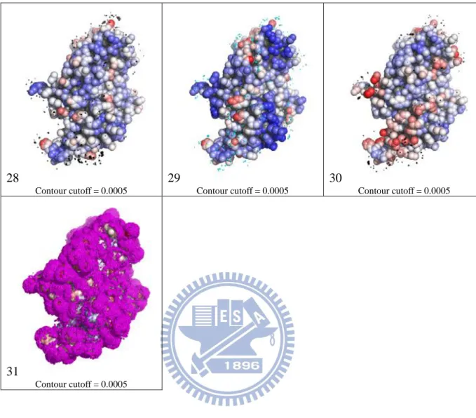
28 Contour cutoff = 0.0005 29 Contour cutoff = 0.0005 30 Contour cutoff = 0.0005 31 Contour cutoff = 0.0005

Figure 1 – Probability density maps and encoded features of human vascular endothelial growth factor A (VEGF). Structure of VEGF is extracted from PDB ID 2FJG chain V and W. Number 1 to 31 in each cell of the table corresponds to each of the interacting atom types defined in Table 1 of the main text. The PDMs are shown in contours colored according to the interacting atom type: cyan for nitrogen, black for carbon, and magenta for oxygen. The contour level is set to 0.0005. Color spectrum of protein atoms in each cell are based on the corresponding ai,j values. Solvent inaccessible atoms are colored in gray. Interactive 3-D graphic presentation of the PDMs can be viewed from the web server http://ismblab.genomics.sinica.edu.tw/ > gallery.

2.2 Machine learning for probability density maps

(PDMs) on protein surfaces

2.2.1 PDM-based attributes as inputs for machine learning

algorithms

One machine learning model was trained for each of the 30 protein atom types (atom types 1~30 in Table 1). The input attributes for each of the machine learning models were calculated from the PDMs on the protein surface. For each protein atom i, the PDM values for interacting atom type j associated with the grids within 5 Å radius centered at the atom i were summed and associated with the center of the atom as Si,j:



  r_ik A k k j j i g S _, , 5 _, (2)

where ri,k is the distance between atom i to a grid point k; gk,j is the PDM value of atom type j at grid point k.

The distance-weighted sum (Ai,j ; j=1~31 for the 31 interacting atom types 1~31 in Table 1) over Sk,j for atoms k within 10Å from atom i was calculated with Equation (3).





  _       ₁₀ 2 , 2 , 10 , , , _, , n i k i d n in k i d k k j j i j i d d S S A (3)

where Si,j is defined in Equation (2); di,k is the distance between atom i and atom k; di,n is the distance between atom i and atom n. Ai,j encodes complementarity information on interacting atom type j over a circular protein surface patch centered at atom i on the

protein. The 32nd attribute for the atom i was the fraction of the space not occupied by the van der Waals volume of the protein in the 10 Å sphere centered at the atom i.

The attributes ai,j (j=1~31 for the 31 interacting atom types in Table 1, and j=32 for the geometry attribute) associated with protein atom i as inputs for the machine learning algorithms were scaled between 0 and 1. Equation (4) shows the calculation of ai,j from Ai,j (j=1~32):

if Ai,j > Mmax,j then ai,j=1; otherwise,

if Ai,j < Mmin,j then ai,j=0; otherwise,

j j j j i j i M M M A a min, max, min, , ,    (4)

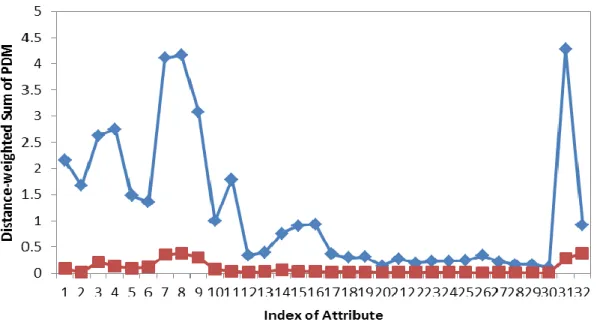
where Mmax,j is the median of the distribution of the maximal Ai,j from each of the proteins in the S432 non-redundant protein data set (see below) and Mmin,j is the median of the distribution of the minimal Ai,j of the same dataset. Figure 2 shows the plots of Mmin,j and Mmax,j against the 32 attribute types.

Figure 2 – Mmin,j (in square symbols) and Mmax,j (in diamond symbols) against the 32 attribute types. The maximum and minimum Ai,j values were derived from each protein in S432 and the medians of the maximum (Mmax,j j=1~32, shown in diamond symbols) and the minimum (Mmin,j j=1~32, shown in square symbols) are plotted against the attribute index. These values were used for normalization of Ai,j (Equation (4)).

2.2.2 Datasets

Three datasets were downloaded from the SPPIDER website [23]. These data sets include a training set, S435, a test set, S149, and an unbound dataset, S21a. We made several modifications to the datasets as the following: Chain A of PDB ID 1GY9 was removed because the complex described in Elkins et al. [48] could not be found in the current PDB. Chain A and C of PDB ID 1DF9 were removed since the records were obsolete. By removing the three proteins from S435, we obtained a dataset named S432. For the independent test set, seven proteins were removed for the following reasons: Chain A and B of PDB ID 1NRJ were removed because they already existed in the training set. Chain

K and L of PDB ID 1N13, chain D of PDB ID 1NF3, and chain D of PDB ID 1L9W were removed because they were identical to chain A and B of PDB ID 1N13, chain C of PDB ID 1NF3, and chain A of PDB ID 1L93 in the training set, respectively. Chain A of PDB ID 1PUG was removed because it was a hypothetical protein. By removing seven proteins from S149, we obtained the independent test set S142. For the unbound dataset, chain A of PDB ID 1GQN and chain A of PDB ID 1RZX were removed because they were identical to chain A of PDB ID 1L93 and chain C of PDB ID 1NF3 in the training set, respectively. Chain A of PDB ID 1J8B was removed because it was a hypothetical protein. Chain A of PDB ID 1NX6 was removed because its interface was engineered with two insertions compared to its bound state protein, chain A of PDB ID 1T4B. By removing the four proteins from S21a, we obtained the unbound dataset S17a.

In order to test the performance of the predictors devised in this work with other comparable predictors in the public domain, we downloaded protein complex structures released in 2011 from PDB website with the following criteria: 1) resolution is less than 3.0 Å , 2) chain length is greater than 100 amino acids, 3) entry has two subunits in biological ensemble, 4) entry does not have DNA, RNA, ligands, or modified residues, 5) there is no missing atom in the PDB files, and 6) pairwise sequence identity between any two proteins is less than 30%. The protein chains were further filtered to ensure none of them share greater than 30% sequence identity to proteins in S432, the training set used in this work as described in the previous paragraph. This set of 58 protein chains, denoted S58, was used as the test set for the comparison of prediction capabilities among different PPI site prediction servers.

2.2.3 Determining biologically relevant PPI sites

All PDB chain records in the three datasets above were checked with PQS (protein quaternary structure) server [49] to determine the biologically relevant PPI sites, so that crystal packing interfaces were removed and biological units were reassembled from asymmetric units. PPI sites at atomistic level were defined with the difference of solvent accessible surface area (dSASA) upon complex formation by NACCESS software [50] as below. i u i c i u i SASA SASA SASA dSASA , , ,   , (5)

where SASAu,i and SASAc,i are the SASA of atom i in the uncomplexed and complexed state, respectively. An atom i was defined as a PPI site atom when dSASAi is greater than 0.

2.2.4 Artificial neural network (ANN)

The standard feed-forward back-propagation neural network [51] was used to learn the weight of the network by employing gradient descent to minimize the sum of squared error between the network output values and the target values. The input layer consisted of 32 nodes for the input attributes described in Equation (4). The only hidden layer contained 15 nodes. The output layer had a single node with the activity value between 0 and 1, matching the negative and positive cases respectively for the atoms in PPI sites as defined in Equation (5). Sigmoid function, denoted as sf, was used as the transfer function for the hidden and output layers of of the ANN network.

1 )] x exp( 1 [ ) x ( sf     (6)

As an alternative to the more common Levenberg-Marquardt back-propagation training algorithm [52], the very high speed resilient back-propagation (RPROP) training technique was used [53, 54]. Resilient propagation is capable of automatic adjustment for learning rate and momentum. It has the advantage of faster convergence while requiring less manual determination of network parameters. Each of the ANN models was trained for 1000 iterations. During training, the model was tested on validation set after every ten training iterations. The number of training iteration which yielded the best MCC (see below for MCC definition) on the validation set was used to determine the predictors. The open source java-based neural network library ENCOG was used for the implementation.

2.2.5 Support vector machines (SVM)

The details of the standard SVM methodology implemented with LIBSVM package has been described previously [33]. In brief, the SVM is a two-class classification approach with a maximized-margin hyperplane, where margin is the distance from the separating hyperplane to the closest data point [55, 56]. The cost (c) and gamma (γ) parameters of the SVM were optimized with grid searching for the optimal MCC using only the training dataset.

2.2.6 Bootstrap aggregation (BAGGING)

Since non-binding atoms in the training set greatly outnumbered binding atoms, ordinary machine learning algorithms would produce learning biases without suitable treatment.

The methodology included multiple predictors to produce an ensemble of prediction results [57]. Each individual classifier in the predictor ensemble was trained with a different sampling (bag) of the training set, and the final prediction was calculated by averaging with equal weight the output values from the predictors [58]. In each bag, all of the positive cases were included, along with randomly sampled negative cases that were 1.5 times as many as positive cases. The bag number was set to ten, which balanced the need for effectiveness and training efficiency. All the ten bags were used to train either a set of ANN models (named ANN_BAGGING) or a set of SVM models (named SVM_BAGGING).

The machine learning parameters can be downloaded from the web-server http://ismblab.genomics.sinica.edu.tw/ >Download. The attributes ai,j (j=1~31 for the 31 interacting atom types in Table 1, and j=32 for the geometry attribute) associated with protein atom i for all proteins in the data sets S432, S142, S17a, S58 can be downloaded from the same web-server.

2.2.7 Prediction capacity benchmarking

The prediction capabilities of the machine learning models were benchmarked by accuracy (Acc), precision (Pre), sensitivity (Sen), specificity (Spe), F-score, and Matthews correlation coefficient (MCC) [59].

FN FP TN TP TN TP      Acc (7)

FP TP TP   Pre (8) FN TP TP   Sen (9) FP TN TN   Spe (10) Sen Pre Sen Pre 2 score -F     (11) ) )( )( )( ( MCC FN TN FP TN FN TP FP TP FN FP TN TP         (12)

where TP is the number of true positives; TN the number of true negatives; FP the number of false positives; and FN the number of false negatives. Sensitivity (also known as recall) can be viewed as a measurement of completeness, whereas precision is a measurement of exactness or fidelity. MCC, as a measurement of the quality of two class classifications (positive and negative), is generally regarded as a balanced measurement which can be used even if the classes are of very different sizes. Its value ranges between -1 and 1; random correlation gives MCC of zero while perfect correlation yields MCC of one.

2.2.8 Prediction confidence level

Prediction activity (ANN_BAGGING) or probability (SVM_BAGGING) with value ranging from 0 to 1 from the output of the machine learning algorithm was normalized to prediction confidence level so that the prediction results from different machine learning models can be compared on a level ground. For each of the 30 protein atom types, the

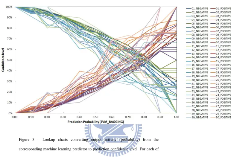
machine learning outputs from the validation sets were sorted into bins of interval 0.1. The prediction confidence level for each of the bins was calculated as the fraction of the true positives over the total number of predictions in the bin. In the end, lookup-tables for output-confidence relationships were constructed; the machine learning outputs can be converted to prediction confidence levels with these lookup tables. Figure 3 shows the relationships between machine learning outputs and the prediction confidence levels for each of the trained machine learning models.

(a )

Figure 3 – Lookup charts converting output activity (probability) from the corresponding machine learning predictor to prediction confidence level. For each of the 30 protein atom types, the machine learning outputs from the validation sets were sorted into bins of interval 0.1. The confidence level of each of the bins was calculated as the fraction of true positive over the total number of predictions in the bin. The panels (a) and (b) are derived from ANN_BAGGING and SVM_BAGGING predictions respectively. In each of the panel, two sets of curves are shown; one set for the prediction confidence level described as above (i.e., the positive prediction confidence); the other set for the negative prediction confidence. The sum of the positive prediction confidence level and the negative prediction confidence level equals to one.

2.2.9 Five-fold cross validation and independent test

Five-fold cross validation was performed for each of the 30 protein atom types in the S432 dataset. Each dataset was randomly divided into 5 equal portions with similar distributions of positive and negative cases. One portion of the dataset was selected as test set, another one portion as validation set, and the rest as training set. The training set was used to train the models, and the validation set was used to optimize the prediction parameters so as to achieve the best predictive capability without over-fitting. The optimized models were then benchmarked by the test set. The process took turns to benchmark prediction accuracy on the 5 non-overlapping test sets with the predictors optimized with the corresponding training and validation set. The accuracy benchmarks were the averaged results from the 5-fold cross validation.

For each of the predictors, an optimal threshold for the output activity value was determined with the validation set. Positive predictions have the output activity values greater than or equal to the threshold; the negative predictions have the output activity values smaller than the threshold. With these thresholds, the TP, TN, FP, and FN in Equations (7)~(12) were determined and the accuracy benchmarks were calculated. The thresholds for the predictors of all 30 atom types were determined to optimize the MCC for the predictions with the validation set.

Five predictors for each protein atom type were optimized after performing the 5-fold cross validation on the S432 dataset. The predictors which yielded the best testing performance were assessed in the independent test with S142, S17a, and S58 dataset.

2.3 Prediction of patches of atoms as protein-protein

binding sites

A protein-protein binding site was predicted by a cluster of surface atoms predicted as positive cases with high prediction confidence level. Protein surface atoms in PPI sites with prediction confidence level greater than 60% were used as cluster centers to include neighboring surface atoms within radius of 11 Å . Within each of the surface patches, all the surface atoms with the confidence level for positive prediction greater than 20% were included in the tentative patch of atoms as a PPI site. If the pairwise distance of any two seeds was within 10 Å , the two corresponding patches were merged as one patch. The parameters were optimized for residue-based prediction accuracy with the validation set.

2.4 Residue-based predictions for the PPI sites

To facilitate comparison of this work with previous methods predicting binding sites at the residue level, a heuristic procedure was used to transform the atom-based binding site predictions as described in the previous paragraph into binding site predictions at the residue level: only the residues with more than 30% of the surface atoms (SASAu>0) included in the atom-based binding patch were considered as positive residues of the residue-based patch. Similarly, actual PPI sites at the residue level were defined by patches of positive residues, each of which has more than 30% of the surface atoms (SASAu>0 in the uncomplexed structure) on the residue defined as PPI atoms (dSASA>0, as shown in Equation (5)). This definition enabled the comparison of prediction results with actual binding sites at the residue level. The percentage parameter was optimized for

residue-based prediction accuracy with the validation set.

2.5 Computational efficiency for predicting PPI sites in

a typical protein

The building of PDMs for a typical protein of 200 residues with Intel Xeon X5650 (2.67GHz) CPU is around 50 minutes with single thread and around 23 minutes with two threads. The following procedures for generating input attributes and for predicting with machine learning models take less than 20 seconds.

2.6 Mann-Whitney U-test

Mann-Whitney U-test is a non-parametric statistical method to test whether two groups of numerical values come from identical continuous distributions of equal medians – increasing p-value indicates decreasing difference of the two distributions and p-value of 1 indicates that the two distributions are statistically indistinguishable. The Mann-Whitney U-tests were carried out with the statistic tool ranksum in MATLAB (http://www.mathworks.com/help/toolbox/stats/ranksum.html).

2.7 Web site

Predictions can be submitted to the webserver

http://ismblab.genomics.sinica.edu.tw/. All the benchmark results can also be accessed in interactive graphic presentations from the same web address above.

Chapter 3

Results and Discussions

3.1 Statistical analysis of physicochemical

complementarities in known PPI interfaces

It has been well-established that geometrical and physicochemical complementarities are critical determinants in PPI interfaces [5]. The amino acid preferences and packing density for PPI core interfaces resemble those of protein interior [4, 60]. The physicochemical complementarities among interface residues are characterized by hydrophobic interactions in the core interface regions and polar interactions in the rim regions of the interfaces [2-4, 7, 61, 62]. Based on the general description of typical PPI interfaces, we hypothesized that the distribution patterns of the non-covalent interacting atoms on a PPI surface should provide abundant information in distinguishing PPI surface regions from non-PPI surface regions.

Figure 4 demonstrates the validity of the hypothesis above. The physicochemical complementarities around the protein surface atom i were simulated with the PDMs of non-covalent interacting atoms and were described with the 32 numerical features calculated with Equation (2) (i.e., Ai,j for interacting atom type j=1~31 as shown in Table 1; j=32 derived from protein surface geometry). The matrix element (j,i) in Figure 4 shows the Mann-Whitney U-test result for the two groups of Ai,j: one group of Ai,j was calculated for the interacting atom type j around the surface atom type i in the known PPI

sites on proteins in the S432 dataset and the other group was calculated for the same interacting atom type around the non-PPI site atom type i in the same dataset. The matrix elements showing decreasing p-value substantially less than the statistical threshold of 0.025 are colored in red with increasing depth. These U-test p-values reflect the significant statistical differences in the attributes calculated from the PDMs or surface geometry between the protein surface atoms in known PPI sites and the atoms outside known PPI sites.

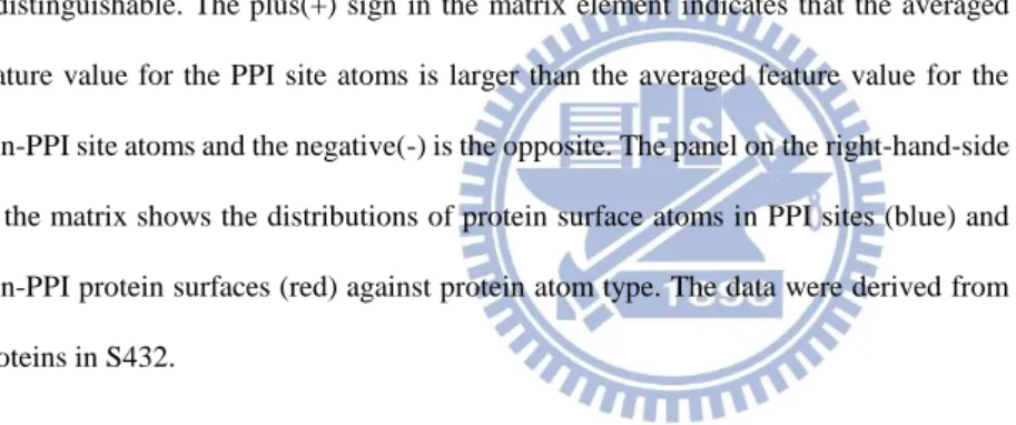
Figure 4 –Mann-Whitney U-tests for the distributions of numerical attributes around protein surface atoms. The y-axis of matrix shows the atom type index (i=30 protein atom types shown in Table 1) and the x-axis shows the j index for the 32 Ai,j features, where j=1,31 represents the 31 interacting atom types shown in Table 1 and the 32nd feature reflects the local geometry of the protein surface. The matrix element (j,i) shows the Mann-Whitney U-test p-value in color-code for the two groups of Ai,j : one group of Ai,j was calculated for the attribute type j around the surface atom type i in the known PPI sites on proteins in the S432 dataset and the other group was calculated for the same attribute type around the non-PPI site atom type i in the same dataset. The p-values were calculated with the Mann-Whitney U-test implemented as the function ranksum in MATLAB. Two sets of data were input to the function and the output p-value is the probability for the two distributions of data to be statistically indistinguishable. The plus(+) sign in the matrix element indicates that the averaged feature value for the PPI site atoms is larger than the averaged feature value for the non-PPI site atoms and the negative(-) is the opposite. The panel on the right-hand-side of the matrix shows the distributions of protein surface atoms in PPI sites (blue) and non-PPI protein surfaces (red) against protein atom type. The data were derived from proteins in S432.

3.2 Consistency of the U-tests of the physicochemical

complementarity features with previous statistical

observations

The U-test results shown in Figure 4 are comparable with general PPI site characteristics from previous statistical observations. Space around the main chain atoms (rows of y=1~4) in PPI sites are enriched with higher densities of interacting backbone carbonyl group (x=2,4) and are neighbored by higher densities of interacting hydrophobic and aromatic carbons (x=6~9), while the interacting charged atoms (x=11, 15~16, 25~28) are largely depleted near the main chain atoms in the PPI sites. This is in agreement with the

observation that main chain atoms are frequently used in polar interactions in PPI [3]. In particular, the carbonyl oxygen (row of y=4) is most frequently used in hydrogen bonding in PPI sites [3]. Aliphatic and aromatic carbons (rows of y=6~9) in PPI sites are surrounded with high density of interacting aliphatic carbons, aromatic carbons, and atoms from Met and His (x=6~9,18~25, 27~30), while charged interacting atoms (x=11, in particular x=26 for Lys Nz) are also depleted in the PPI sites. But, interestingly, Arg (x=15,16) remains favorable in the PPI sites near the aromatic carbons (y=9), in particularly with atoms from Trp (y=18,24,30). Arg also interacts with carboxyl oxygen (y=11) more in the PPI sites. This is largely in consistent with the knowledge-based pairwise potentials devised with protein-protein interaction datasets [5, 62]. The sulfur atom of Cys is highly enriched in the PPI sites as interacting atoms (column x=20), in good agreement with the high interface propensity for Cys [63]. Interacting water molecules (column x=31) are more dense in PPI sites near polar atoms (y=1~4,10~13,16~17). This is in consistent with the statistical survey by Rodier et al. [8], suggesting that water molecules in the PPI interfaces play important roles in protein complex formation. The results in the last column (column of x=32) suggest that PPI sites are more flat or convex than non-PPI surfaces, which is in good agreement with the survey by Jones and Thornton [63]. Although the dataset did not provide enough statistical resolution for rows of y=18~30 (see the dataset distribution indicated by the histogram next to the U-test matrix), the consistencies listed above nevertheless suggest that the distribution patterns of the non-covalent interacting atoms predicted with the PDMs on PPI interfaces can provide statistical characteristics in distinguishing the known PPI sites from the other protein surface regions that have not been known to bind to

proteins. Since the PDMs were derived from known protein structures, the correlation between the PPI interface features (Figure 4) predicted with the PDMs and those derived from surveys of PPI interfaces also implies that both protein folding and binding are governed by similar energetic principles.

3.3 Atom-based PPI site predictions with machine

learning models based on physicochemical

complementarity features

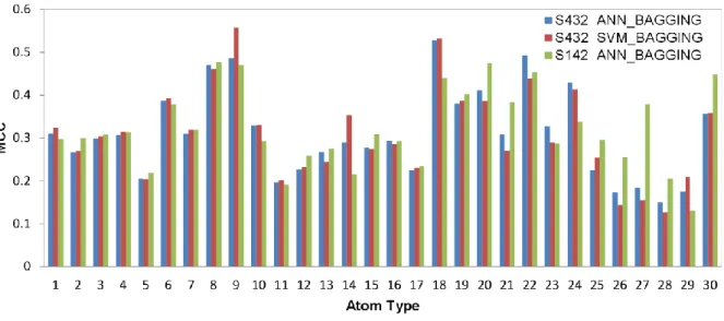
The results in Figure 4 indicate that the 31 features calculated with PDMs (a set of example PDMs on a protein are shown in Figure 1) and the 32nd feature based on the surface atom local geometry for each of the 30 protein atom types can be used as effective attributes in training machine learning models for PPI site predictions. Machine learning algorithms ANN_BAGGING and SVM_BAGGING were trained for each of the 30 protein surface atom types with five-fold cross validation on the S432 dataset as described in the Methods section. The atom-based MCCs for the five-fold cross validation for each of the atom types are summarized in Figure 5. The benchmarks for the prediction models are shown in Table 3. The differences of the averaged performance for the two machine learning algorithms are essentially indistinguishable (Figure 5 and Table 3), and thus only the ANN_BAGGING models with the best performance were used to benchmark on the S142 dataset as an independent test. The benchmark results on the independent test are compared with the five-fold cross validation in Figure 5 and in Table 3. The benchmark results for the independent test were comparable with the five-fold cross validation results, indicating that the machine learning predictors can be generalized to predict PPI sites on

protein surfaces of unknown interaction partners. Figure 5 shows that the prediction models for the atom types from hydrophobic residues with aliphatic and aromatic side chains (atom type index=8,9,18~24,30) were predicted with relatively higher accuracies than the atom types from main chain and hydrophilic side chains. This suggests that the core PPI interfaces composed of hot-spot residues (except Arg) are more distinguishable as PPI sites in comparison with the surrounding rim regions populated with higher percentage of polar groups.

Figure 5 – Atom-based prediction accuracies for each of the 30 protein atom types. The x-axis represents indexes for the 30 atom types shown in Table 1. The y-axis shows averaged two-class prediction MCCs from the 5-fold cross validation of the ANN_BAGGING and SVM_BAGGING predictors trained and tested for each of the specific protein atom type with the S432 dataset. The prediction MCCs for the independent test with ANN_BAGGING on the S142 dataset are also shown for comparison.

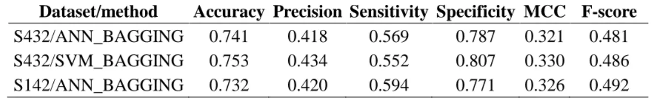
Table 3 – Benchmarks for atom-based PPI site predictions. Five-fold Cross validation was performed on the S432 dataset with ANN_BAGGING and SVM_BAGGING. Independent test was performed on the S142 dataset with the best ANN_BAGGING predictors from the five-fold cross validation. The benchmark measurements are defined in Equations (7)~(12).

Dataset/method Accuracy Precision Sensitivity Specificity MCC F-score

S432/ANN_BAGGING 0.741 0.418 0.569 0.787 0.321 0.481 S432/SVM_BAGGING 0.753 0.434 0.552 0.807 0.330 0.486 S142/ANN_BAGGING 0.732 0.420 0.594 0.771 0.326 0.492

The PPI surface patches on protein surfaces were predicted by combining the machine learning predictions for each of the surface atoms. The activity (probability) outputs from the machine learning models were first converted into prediction confidence levels so that surface atoms with high confidence level predictions can be clustered into surface patches as PPI sites (see Methods). Figure 6 shows a few examples of protein surface PPI site predictions, compared side-by-side with actual PPI sites, with various prediction accuracies (residue-based MCC ranging from 0.7 to 0.1). The complete set of prediction results on the proteins from the training and test sets can be viewed with interactive 3-D structural presentation from the web server http://ismblab.genomics.sinica.edu.tw/> benchmark > protein-protein.

Figure 6 –Visualization of prediction results for example protein targets with different prediction accuracy. Panels (A) to (D) demonstrate four proteins with two-class prediction MCC of 0.650, 0.454, 0.262, and 0.107, respectively. The target proteins were selected from the S142 dataset. The predictions were carried out with the best ANN_BAGGING model from the 5-fold cross validation on the S432 dataset. In each panel, the left structure shows the atom-based positive prediction confidence level from blue (confidence level of 0) to red (confidence level 1) for each of the surface atoms. The middle structure shows the residue-based predictions. The atoms colored in red were predicted with confidence level greater than 0.6; atoms in orange are the atoms belonging to the residues in the residue-based PPI site prediction but the prediction confidence levels are less than 0.6. The right-hand-side structure shows the actual PPI sites: the PPI surface atoms are colored according to dSASA (see Equation (5)) from blue (dSASA of 0 for atoms not involving in PPI) to red (dSASA of 1 for atoms completely buried in the protein complex). The color-codes are shown at the top of the figure. Atoms not used in prediction (colored in yellow) belong to residues with incomplete phi and psi angles, as in the N-termini or C-termini of proteins. The non-surface atoms are colored in gray. The complete prediction results can also be viewed in color-coded 3-D protein structures from the web server http://ismblab.genomics.sinica.edu.tw/> benchmark > protein-protein.

3.4 Residue-based PPI site predictions with machine

learning models based on physicochemical

complementarity features and the comparison of

the prediction benchmarks among comparable

predictors

Residues in the predicted PPI surface patches were predicted based on the atom-based PPI site predictions (see Methods) and were benchmarked with the residues in actual PPI sites. The example residue-based PPI site predictions are also compared side-by-side with the

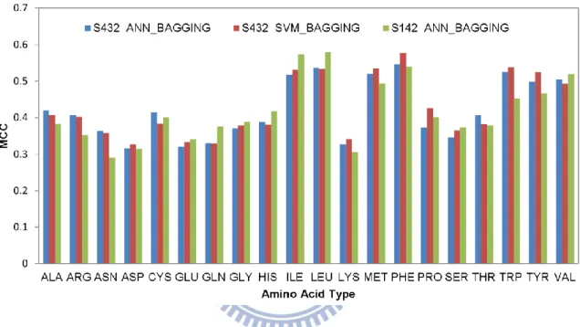
atom-based predictions and the actual PPI sites in Figure 6. The residue-based MCC for each of the amino acid types are shown in Figure 7. The accuracy benchmarks are summarized in Table 3. Again, the two machine learning algorithms are comparable in terms of the prediction performance (Table 4 and Figure 7). The generalized prediction capacity of the ANN_BAGGING models was demonstrated with the results of the independent test, for which the results were essentially indistinguishable from the results of the five-fold cross validation as shown in Figure 7 and Table 4. The prediction results can also be viewed in color-coded 3-D protein structures from the web server http://ismblab.genomics.sinica.edu.tw/> benchmark > protein-protein.

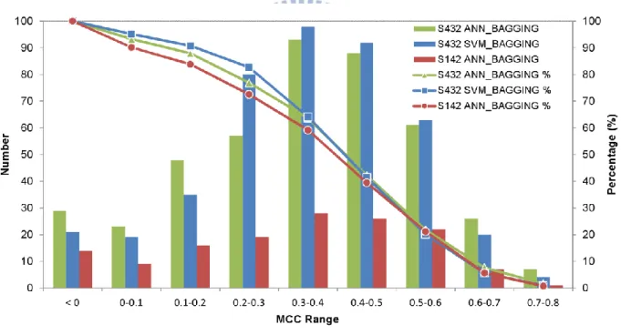
The distribution of prediction accuracy for proteins in the S432 and S142 dataset are shown in Figure 8, for which the overall benchmark results are summarized in Table 4. The independent test (MCC=0.423) for the residue-based PPI site predictions, as shown in Table 4, can be compared with previous publications based on the same training and test datasets. Porollo et al. [23] developed SPPIDER predictor for PPI site residue predictions with essential the same training and test datasets based on a combination of structural and sequence features. Their residue-based prediction MCC for the independent dataset is 0.42. In another work, a detailed analysis of the sequence and structural attributes on the same training and test datasets has concluded that the best performance for independent PPI site residue-based predictions yielded MCC of 0.37 on the same test set [9]. By taking away the evolutionary information from the prediction inputs, the MCC dropped to 0.34. Hence, the PPI site predictions based on the physicochemical complementarities derived from the PDMs on the protein surfaces are currently the best