多重輸入多重輸出正交分頻多工空間分割存取下鏈系統在通道估計錯誤下之共同波束設計

國 立 交 通 大 學

電信工程學系

碩 士 論 文

多重輸入多重輸出正交分頻多工空間分割存取下鏈系統在

通道估計錯誤下之共同波束設計

Joint Tx/Rx MMSE Beamforming Design for Multi-user

MIMO-OFDM SDMA Downlink System under Channel

Estimation Error

研究生：林偉凱

指導教授：紀翔峰

多重輸入多重輸出正交分頻多工空間分割存取

下鏈系統在通道估計錯誤下之共同波束設計

研究生：林偉凱 指導教授：紀翔峰 博士

國立交通大學

電信工程學系碩士班

摘要

近年來，多重輸入多重輸出正交分頻多工空間分割多重存取技術已成為現今 寬頻無線網路系統的主要方法之一，在此論文中，我們將著重此技術在多用戶下 鏈系統中的波束設計及應用。 過去，已有不少的文獻研究收發機共同波束設計在多重輸入多重輸出系統的 應用，然而在這些研究都考慮單一用戶系統，此外，他們也都假設在有完美的通 道估計來設計。然而，這個假設在實際通訊系統中是不存在的，故在此論文中， 我們將針對多用戶系統，在通道估計有誤差的情況下，提供一個收發機共同波束 設計方法能有效抵抗通道錯誤所造成的系統效能損失。 收發器共同波束技術能將原本空間上互相干擾的多重輸入多重輸出系統轉

換成一個子通道間互相獨立不干擾的等效系統。而在我們所提出的多重輸入多重 輸出正交分頻多工空間分割多重存取下鏈系統中，藉由在傳送端利用零空間技 巧，我們能將多用戶系統轉換為一個用戶間互相獨立的系統，如此便可將文獻中 的單一用戶收發機共同波束技術應用在每個獨立用戶上。此外，在有多路徑的頻 率選擇通道下，我們將採用正交分頻多工技術應用在上述系統中。 進一步的，先前所提到的設計方法皆假設在有完美的通道估計條件下，然而 在實際系統上通道估計通常會有誤差，此誤差將造成顯著的系統效能損失，此損 失可歸咎於因為不完美零空間矩陣所造成多用戶間互相的干擾，以及因為不完美 收發機共同波束設計所造成每個用戶本身資料串之間的干擾。在此論文中，我們 將考慮多用戶多重輸入多重輸出正交分頻多工空間分割多重存取下鏈系統在通 道估計有誤差的情況下，提供一個較能抵抗因為通道錯誤所造成系統效能損失的 收發機共同波束設計。最後，我們利用電腦模擬來評估比較系統效能。

Joint Tx/Rx MMSE Beamforming Design for

Multi-user MIMO-OFDM SDMA Downlink

System under Channel Estimation Error

Student：Wei-Kai Lin Advisor：Dr. Hsiang-Feng Chi

Department of Communication Engineering

National Chiao Tung University

Hsinchu, Taiwan

Abstract

The techniques of MIMO-OFDM SDMA have recently considered one of the candidates for the broad-band multiple-access wireless systems. In this thesis, we focus on the research of beamforming in the applications of multi-user MIMO-OFDM SDMA downlink wireless system.

Many researchers have used the joint Tx/Rx beamforming approach in the MIMO systems. However, they only considered the single user system. In addition, their methods are proposed under the perfect channel estimation assumption, which is no true in the real world. In this thesis, we will aim at multi-user MIMO SDMA systems to propose a MMSE beamforming algorithm, which has better immunity to

the channel estimation errors than the previously published methods.

The joint Tx/Rx beamforming technique can transform a mutually cross-coupled MIMO transmission system into a set of independent eigen subchannels so that subchannel signal can be decoded without the interference from other antennas. In our proposed MIMO-OFDM SDMA downlink system, by using null-space technique in the base station (Tx side), the multi-user MIMO downlink system can be simplified into several independent single user MIMO subsystems. The MMSE beamforming algorithm is further applied to each single user MIMO subsystem achieving the spatial diversity gain. In addition, to combat the frequency-selective channel caused by multi-paths, we focus the aforementioned problems in the MIMO-OFDM systems.

However, all the previously proposed methods are derived under the assumption of perfect channel estimation. But in real wireless systems, the channel estimate always contains estimation errors which may cause significant performance degradation when these methods are used. The performance loss can be imputed to the multi-user interference induced by the imperfect null-space matrix and the inter-stream interference caused by imperfect Tx/Rx beamforming. In this thesis, without the assumption of perfect channel estimation, we will consider the joint Tx/Rx beamforming design for multi-user MIMO-OFDM SDMA downlink system which is more robust to channel estimation error than the previous methods. Finally, the performance of the proposed schemes will be evaluated by computer simulations.

誌謝

光陰似箭，短短兩年碩士班的研究生涯，以此論文之告成，即將劃上句號。 在這兩年裡，首當感謝指導教授 紀翔峰老師於研究以及論文上給予充分且詳實 的指導與教誨鼓勵，令學生受益匪淺。 其次感謝交通大學電信系教授 吳文榕老師以及教授 黃家齊老師擔任口試 委員的指導與建議，在此也表現由衷的感謝。 衷心的感謝實驗室的學長、同學及學弟們給予研究上的指導幫助才能順利完 成碩士生涯，也共同度過許多快樂的時光，更有難忘的回憶，謝謝你們。 最後，要特別感謝我的父母以及家人還有女友及其家人，特別是父母的辛苦 栽培以及默默付出，還有女友平時的照顧，使得我得以全心投入學業。再次衷心 的謝謝以上諸位，由於你們的幫忙，此論文得以完成，衷心感謝。 僅以此篇論文獻給對我付出關心的你們。 民國九十五年八月 研究生林偉凱謹識於交通大學

Contents

中文摘要………1 英文摘要………3 誌謝………5 Contents……….6 List of Figures………...9 1 Introduction……….11

1.1 MIMO-OFDM Based System………..11

1.1.1 Overview of MIMO System…...………..12

1.1.1.1 MIMO Channel Models………....12

1.1.1.2 Properties of MIMO Channels………..14

1.1.1.3 Tradeoffs Between Gains………..18

1.1.2 Introduction of OFDM Technology………...19

1.1.3 MIMO-OFDM System…...………..22

1.2 Motivation………24

1.3 Thesis Organization………...………...26

2 Joint Tx/Rx MMSE Beamforming Design for Single User MIMO-OFDM Downlink System with Perfect CSI...……….27

2.1 Introduction……….27

2.2.1 Single Carrier Flat-fading Case………... 28

2.2.2 OFDM-based Case……… 30

2.3 Joint Tx/Rx Beamforming Design for Single User Case………32

2.3.1 Problem Description……….. 32

2.3.2 Optimum Transmit and Receive Beamformings………... 33

2.3.2.1 Lagrange Multiplier Method………... .33

2.3.2.2 Two Step Method………...………...36

2.3.3 Equivalent Decomposition of MIMO-OFDM system………....37

2.4 Conclusions…………...………39

3 Joint Tx/Rx MMSE Beamforming Design for Multi-user MIMO-OFDM SDMA Downlink System with Perfect CSI...………41

3.1 Introduction………...41

3.2 Joint Tx/Rx Beamforming MIMO SDMA System Models……….43

3.2.1 MIMO SDMA under Single Carrier Flat-fading Channel…………..43

3.2.2 MIMO-OFDM SDMA………....44

3.3 Joint Tx/Rx Beamforming Design for Multi-user Case………...44

3.3.1 Null-space Constraint Design……….44

3.3.2 Joint Tx/Rx Design with Null-space Constraint……….47

3.3.3 Derivation of The Joint Tx/Rx Design with Null-space Constraint...49

3.4 Simulation Results and Comments………..52

4 Robust Design of Joint Tx/Rx MMSE Beamforming with Excellent Channel Estimation Error Immunity for Multi-user MIMO-OFDM SDMA Downlink

System...56

4.1 Introduction………..56

4.2 Robust Design of Joint Tx/Rx Beamforming...……..58

4.2.1 Problem Description………...58

4.2.2 Robust Designs………...61

4.2.2.1 Robust Design Against MUI……….61

4.2.2.2 Robust Design Against Imperfect Beamformings…………63

4.2.2.3 Robust Design Using Moving Average Method…………...65

4.3 Simulation Results and Comments………..66

4.4 Conclusions...………72

5 Conclusions and Perspective………..74

5.1 Conclusions………..74

5.2 Perspective………...…75

List of Figures

Figure 1-1 A MIMO system with M transmit and N receive antennas under flat-fading channel……….12

Figure 1-2 A MIMO system with M transmit and N receive antennas under frequency selective channel………...13

Figure 1-3 Beamforming gain obtained from a SIMO system...15

Figure 1-4 Multiplexing gain obtained from a MIMO system ...17

Figure 1-5 Smart antennas overview.……… 17

Figure 1-6 (a) OFDM (b) Conventional MCM...19

Figure 1-7 Classical scheme of an OFDM communication system...22

Figure 1-8 MIMO-OFDM transmit side...22

Figure 1-9 MIMO-OFDM receive side...23

Figure 2-1 Joint Tx/Rx beamforming design for single user MIMO system...29

Figure 2-2 Joint Tx/Rx beamforming processing at transmitter of a single user MIMO-OFDM system…………. 31

Figure 2-3 Joint Tx/Rx beamforming processing at receiver of a single user MIMO-OFDM system... 31

Figure 2-4 The matrix model of a single user MIMO-OFDM system at k-th subcarrier...38

Figure 2-5 Equivalent decomposition of MIMO-OFDM system at k-th subcarrier...39

Figure 3-1 Joint Tx/Rx beamforming design for a multi-user MIMO SDMA downlink system... 43

Figure 3-2 Joint Tx/Rx beamforming design for a multi-user MIMO downlink system with null-space matrix... 44

Figure 3-3 The vertical concatenation representation of a multi-user MIMO channel matrix... 45

Figure 3-4 The horizontal concatenation representation of a multi-user null-space matrix... 46

Figure 3-5 The product of the MIMO channel and the null-space matrix...47

Figure 3-6 Joint Tx/Rx beamforming for multi-user MIMO-OFDM downlink system with null-space matrix... 48

Figure 3-7 Joint Tx/Rx beamforming for multi-user MIMO-OFDM downlink system at transmitter... 48

Figure 3-8 Joint Tx/Rx beamforming for multi-user MIMO-OFDM downlink system at u-th user receiver... 49

Figure 4-1 Joint Tx/Rx beamforming design for multi-user MIMO downlink system under imperfect CSI...57 Figure 4-2 Joint Tx/Rx beamforming for multi-user MIMO-OFDM downlink system with null-space matrix...59

Figure 4-3 Joint Tx/Rx MMSE beamforming design for MIMO-OFDM SDMA system under CSI error 0.075.... 67 Figure 4-4 Joint Tx/Rx MMSE beamforming design for MIMO-OFDM SDMA system under CSI error 0.05... 67

Figure 4-5 Joint Tx/Rx MMSE beamforming design for MIMO-OFDM SDMA system under CSI error 0.025.... 68 Figure 4-6 Joint Tx/Rx MMSE beamforming design for MIMO-OFDM SDMA system under CSI error 0.05... 69

Figure 4-7 Joint Tx/Rx MMSE beamforming design for single user MIMO-OFDM system under CSI error 0.1...70 Figure 4-8 Joint Tx/Rx MMSE beamforming design for single user MIMO-OFDM system under CSI error

0.075……….... 71 Figure 4-9 Joint Tx/Rx MMSE beamforming design for single user MIMO-OFDM system under CSI error

0.05………...71 Figure 4-10 Joint Tx/Rx MMSE beamforming design for single user MIMO-OFDM system under CSI error

---

Chapter 1

Introduction

---

In the recent years, due to the rapid increase in broadband access demand, the wireless system with high data rates and high link quality services has become one of the hot research topics. The MIMO-OFDM system is considered as one of the most promising technologies to provide these services. In this chapter, we will begin with the brief overview of MIMO systems, OFDM technology, and the MIMO-OFDM system. Then, we describe the motivation of the research. Finally, the organization of this thesis will be presented in the end of this chapter.

1.1 MIMO-OFDM Based System

To meet the requirement of high data rates and good link quality, the multiple-input multiple-output (MIMO) orthogonal frequency division multiplexing (OFDM) is considered as one of the promising technologies for broadband wireless communication systems, such as 802.11n and 802.16e. In the following sections, we will briefly introduction the basics of MIMO [1] [2] [3] and OFDM [4] technologies and describe how they can provide high data rate and link quality services. These two technologies are further combined [5] to solve the multi-path channel problem in

broadband wireless systems. Each subcarrier of OFDM system can be treated as a simple flat-fading MIMO channel.

1.1.1 Overview of MIMO System 1.1.1.1 MIMO Channel Models

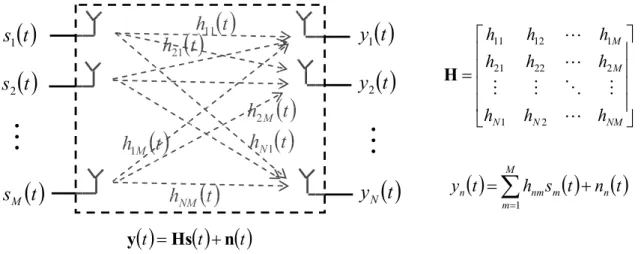
The basic signal model for a single-carrier flat-fading MIMO channel with M transmit and N receive antennas is illustrated in Figure 1-1 where H=

{ }

h_nm is the channel matrix with dimension N×M , s

( )

t =

{

s_m

( )

t

}

is input vector and

( )

t =

{

y_n

( )

t

}

y is output vector. The discrete-time model with matrix form can be wrote as

( )

k Hs

( ) ( )

k n k

y = + (1.1.1.1-1) where y

( )

k =

[

y1

( ) ( )

k ,y2 k ,L,y_N

( )

k

]

T is the receive signal vector,

( )

[

( ) ( )

( )

]

T M k x k x k x k = 1 , 2 ,L,

x is the transmit signal vector, H=

{ }

h_nm is channel matrix with dimension N×M and n

( )

k is noise vector.

( )

t s₁

( )

t s₂

( )

t s_M

M

( )

t y₁

( )

t y₂

( )

t y_N

M

( )

t h₁₁

( )

t h21

( )

t h1_M

( )

t h_NM

( )

t h_N1

( )

t h_2M

Figure 1-1 A MIMO system with M transmit and N receive antennas under flat-fading channel

⎥ ⎥ ⎥ ⎥ ⎦ ⎤ ⎢ ⎢ ⎢ ⎢ ⎣ ⎡ = NM N N M M h h h h h h h h h L M O M M L L 2 1 2 22 21 1 12 11 H

( )

t h s

( )

t n

( )

t y M _n m m nm n =

∑

+ =1

( )

t Hs

( ) ( )

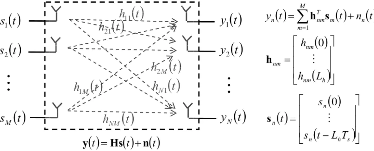
t n t y = +

We now consider the frequency-selective fading channel. The signal model for such environment is shown as following Figure 1-2

( )

t s₁

( )

t s₂

( )

t s_M

M

( )

t y₁

( )

t y₂

( )

t y_N

M

( )

t h₁₁

( )

t h21

( )

t h_1M

( )

t h_NM

( )

t h_N1

( )

t h2_M

where H=

{ }

hT_nm is the MIMO channel matrix with dimensions N×M

(

L_h+1

)

, and

h

L is maximum channel order. The MIMO system can be described by the

discrete-time model as

∑

= − + = L l l k l k k 0 n s H y (1.1.1.1-2) ⎥ ⎥ ⎥ ⎥ ⎦ ⎤ ⎢ ⎢ ⎢ ⎢ ⎣ ⎡ + ⎥ ⎥ ⎥ ⎥ ⎦ ⎤ ⎢ ⎢ ⎢ ⎢ ⎣ ⎡ ⎥ ⎥ ⎥ ⎥ ⎦ ⎤ ⎢ ⎢ ⎢ ⎢ ⎣ ⎡ = ⎥ ⎥ ⎥ ⎥ ⎦ ⎤ ⎢ ⎢ ⎢ ⎢ ⎣ ⎡

∑

= k N k k k M k k L l l NM l N l N l M l l l M l l k N k k n n n s s s h h h h h h h h h y y y , , 2 , 1 , , 2 , 1 0 , , 2 , 1 , 2 , 22 , 21 , 1 , 12 , 11 , , 2 , 1 M M L M O M M L L M (1.1.1.1-3)

Note that when M =1, the MIMO channel reduces to a single-input multiple output (SIMO) channel. Similarly, when N =1 , the MIMO channel reduces to a multiple-input single-output (MISO) channel. When both M =1 and N =1, the MIMO channel simplifies to a simple traditional SISO channel. Following, we will discuss some properties of MIMO channels.

( )

t Hs

( ) ( )

t nt y = +

( )

t

( )

t n

( )

t y M _n m m T nm n =

∑

+ =1 s h

( )

( )

⎥⎥ ⎥ ⎦ ⎤ ⎢ ⎢ ⎢ ⎣ ⎡ = h nm nm nm L h h M 0 h

( )

( )

(

)

⎥⎥ ⎥ ⎦ ⎤ ⎢ ⎢ ⎢ ⎣ ⎡ − = s h n n n T L t s s t _M 0 s

1.1.1.2 Properties of The MIMO Channel

MIMO channels have a number of advantages over traditional SISO channels such as the beamforming (or array) gain, the diversity gain, the interference suppression gain and the multiplexing gain [2] [6]. The beamforming and the diversity gains exist not only in MIMO channels but also in MISO or SIMO channels. However, the multiplexing gain is a unique feature that exists only in MIMO channels. Some gains can be simultaneously achieved while others compete and become a tradeoff [2] [6]. We briefly introduce these gains as follows [2] [6]:

z Beamforming (or array) Gain: Multiple antennas (or array antenna) at transmit or receive terminal coherently combine the signal energy improving the signal-to-noise ratio (SNR) and suppress interference. Therefore, if the bit-error-ratio (BER) of a communication system is plotted with respect to the transmitted or received power per antenna using a logarithmic scale, the beamforming or array gain is easily characterized as a shift of the performance curve due to the gain in SNR.

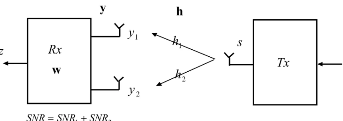
Besides, beamforming is a term traditionally associated with array processing or smart antennas in wireless communication systems where an array antenna can be arranged either at transmitter or at receiver. For illustration purposes, we consider a SIMO system shown in Figure 1-3 with the received signal given by y = sh +n where h is the channel of the desired signal and n is white noise with E

[ ]

nnH =σ2I.

Rx

Tx

s

y

1

y

2

y

w

z

h

1 2

h

h

The receiver uses a beamforming vector w to combine all the elements of y in a coherent way as z=wHy. If the beamvector matches the channel, that is if w=h, the SNR is maximized and given by

SNR = 2 2

σ

h

(1.1.1.2-1) which clearly shows the increase of SNR with respect to using a single receive dimension SNR = 2 2 σ h (1.1.1.2-2) z Diversity Gain: Diversity gain obtained from multiple antennas helps to

combat channel fading and enhance the link reliability. The receiver receives replicas of the information signal through independently fading links, branches, or dimensions occurred by multiple antennas equipped at the transmit or the receive terminal. This type of gain is clearly related to the random nature of the channel and is closely connected to the statistics of channels. If the BER of a communication system is plotted with respect to the transmitted power or the received power per antenna using a logarithmic

2 1 SNR

SNR SNR = +

scale, the diversity gain is easily characterized as the increase of the slope of the performance curve in the low BER region [2]. The basic idea is that with high probability, at least one or more of these links will not be in a fade at any given instant. In other words, the use of multiple dimensions reduces the fluctuations of the received signal and eliminates the deep fades.

Clearly, this concept is suitable for wireless communications where fading exists due to multipath effects and it may not be useful for wireline communications where the fading effect does not exist.

There are three main forms of traditional diversity used in wireless communication systems, temporal diversity, frequency diversity, and spatial diversity. The spatial diversity gain can be obtained from receive and transmit antenna array.

z Interference suppression gain: Interference suppression gain is obtained from multiple antennas equipped at receiver where adaptively combines to selectively cancel or avoid interference and pass the desired signal.

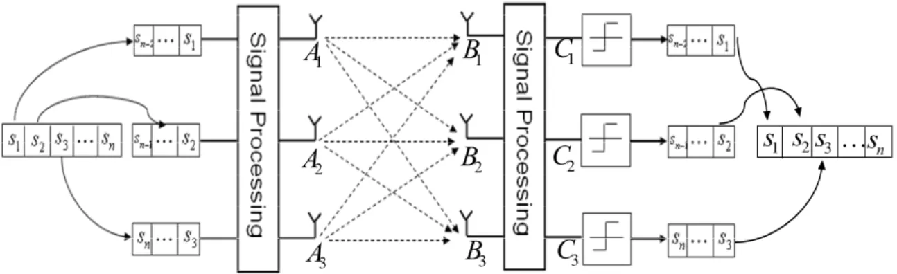
z Multiplexing Gain: Spatial multiplexing gain uses multiple antennas at both ends to create multiple channels and increase of rate, at no additional power consumption. While the beamforming and the diversity gains can be obtained when multiple antennas are equipped at either transmit or the receive side, multiplexing gain requires multiple dimensions at both ends of the link. The basic idea is to exploit the multiple dimensions to create several parallel subchannels within the MIMO channel, which lead to a

transmission of several symbols simultaneously. Figure 1-4 shows the spatial multiplexing gain obtain from a MIMO system.

1

s

s

₂

s

_3L

s

_n 1

A

2

A

3

A

1

B

2

B

3

B

1

C

2

C

3

C

These types of smart antenna can be used to improve coverage, link quality, data rates and system capacity. We summarize the above descriptions inFigure 1-5.

Space-time Processing

Smart Antenna

MISO/SIMO MIMO

Array Gain Interference

Reduction Diversity Gain Multiplexing Gain

Coverage Link Quality Capacity Data Rate

Outdoor

Specular Channel

Indoor Scattering Channel

Figure 1-4 Multiplexing gain obtained from a MIMO system

1.1.1.3 Tradeoffs Between Gains

z Beamforming and Diversity Gains

Beamforming gain is a concept that refers to combine multiple copies of the same signal for a specific channel realization not for the statistics of a channel. However, diversity gain is directly related to the statistical behavior of a channel. With multiple antennas at receive terminal, both array and diversity gains can be achieved at the same time by a coherent combination of the received signals and there is no tradeoff between them. With multiple antennas at transmit terminal, beamforming gain requires CSI (Channel State Information) at the transmitter while diversity gain can be achieved even when the CSI is unknown.

z Beamforming and Multiplexing Gains

Maximum beamforming gain on a MIMO channel implies that only the maximum singular value of the channel should be used. However, for multiplexing gain, the optimum approach is to use a set of the channel singular values according to a water-filling strategy. In other words, maximum beamforming gain requires establishing only a single substream for communication while maximum multiplexing gain requires establishing several substreams at the same time.

z Diversity and Multiplexing Gains

Traditionally, the design of systems has been focused on either extracting maximum diversity gain or maximum multiplexing gain. However, both of these gains can be simultaneously obtained, but there is a fundamental tradeoff

gain is related to the data rate, the tradeoff between them is essentially the fundamental tradeoff between the error probability and the data rate of a system.

1.1.2 Introduction of OFDM Technology

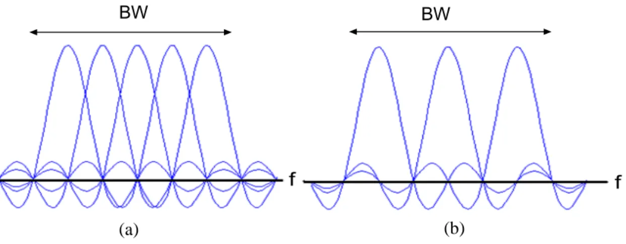
OFDM is a promising technique to achieve high data rate and combat multipath fading effect in wireless communications. OFDM can be thought of as a hybrid of multi-carrier modulation (MCM) and frequency shift keying (FSK) modulation [4]. MCM is the principle of transmitting data by dividing the stream into several parallel sub-streams and modulating each of these data sub-streams onto individual carriers; FSK modulation is a technique which data is transmitted on one carrier from a set of orthogonal carriers in each symbol duration. Orthogonality among these carriers is achieved by separating these carriers by an integer multiple of the inverse of symbol duration of the parallel bit streams. Using OFDM technique, all the orthogonal carriers are transmitted simultaneously. In other words, the entire allocated channel is occupied through the aggregated sum of the narrow orthogonal subbands. Figure 1-6 illustrates the spectral efficiency of OFDM compared to conventional MCM.

f f (b) (a) BW BW

We now briefly describe some fundamental principles of FSK modulation as they pertain to OFDM modulation. The input sequence determines which of the carriers is transmitted by its symbol duration, that is,

( )

t A

(

j f_it

) ( )

t T i = exp 2π Π / s (1.1.2-1) where , / T i f f_i = _c+ i=0,1_K,L−1 (1.1.2-2)

( )

⎩ ⎨ ⎧ ≤ ≤ = Π otherwise , 0 2 2 for , 1 /T -T/ t T/ t

L is the total number of carriers and T is the symbol duration. In order to avoid

that the carriers interfere with each other during detection, the spectral peak of each carrier must coincide with the zero crossing of all the other carriers as depicted in Figure 1-6. Thus, the difference between the center lobe and the first zero crossing represents the minimum required spacing and is equal to 1/T. An OFDM signal is constructed by assigning parallel bit streams to these subcarriers with minimum required spacing, normalizing the signal energy, and extending the bit duration, i.e.,

( )

( ) (

n j ft

)

n L i N N

A

n = x_i exp 2π_i , for 0≤ ≤ ,0≤ ≤

s (1.1.2-3)

where x_i

( )

n is the n-th bit of the i-th data stream. Recall that from the Discrete Fourier Transform (DFT) pairs, the above equation is just the inverse DFT (IDFT) of

( )

n

x_i scaled by A . The output sequence s

( )

n is transmitted one symbol at a time across the channel.

symbol. This makes a portion of the transmitted signal s~ periodic with period L , i.e.:

(

n m

) (

s L n m

)

n-m LCP

s − =~ + − , for ≤

~ _(1.1.2-4) where L is length of CP. Hence the received signal using vector notation is given _CP by

( ) ( ) ( ) ( )

n s n h n n n

y = ~ ∗ +

~ _(1.1.2-5)

where ∗ denotes linear convolution, h is the channel impulse response vector, and

n is the additive noise vector. Now if length of CP is longer than the delay spread of

the channel, received useful part y

( )

n becomes circular convolution one

( ) ( )

n s n _Lh

( ) ( )

n n n

y = ⊗ + (1.1.2-6) where ⊗_L denotes L-point circular convolution. Note that the DFT transform for the convolution theory is based on circular convolution. Hence, the received signal at the k-th subcarrier after DFT results a simple scalar multiplication and can be written as

k k k

k S H N

Y = ⋅ + (1.1.2-7) where Y _k , S_k and H are the k-th subcarrier of DFT of _k y , s and h respectively. Figure 1-7 illustrates the classical scheme of an OFDM communication system. Because of the advantages of OFDM, it becomes a popular transmission scheme for wireless communication systems. For examples, OFDM has been adopted in many standards such as digital audio and video broadcasting (DAB and DVB) and wireless local area networks (WLAN) standards etc.

S/P IFFT (add CP) P/S h(n) + Noise S/P FFT P/S (remove CP)

( )

n s _y

( )

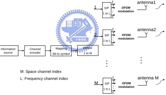
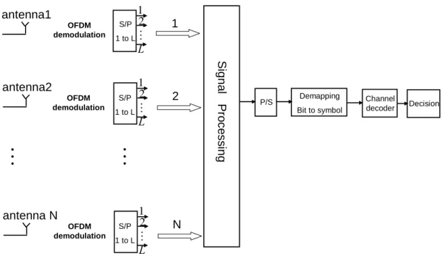
_n Y S 1.1.3 MIMO-OFDM System

After describing the features of MIMO and OFDM techniques, we now combine these two techniques to form MIMO-OFDM systems [5]. Figure 1-8 and 1-9illustrate the basic structure of transmitter and receiver of MIMO-OFDM system respectively.

Information source Channel encoder Mapping Bit to symbol Demux 1 to M S/P 1 to L 1 1 2 LM OFDM modulation antenna1 S/P 1 to L 2 1 2 LM OFDM modulation antenna2 S/P 1 to L M 1 2 LM OFDM modulation antenna M

M

M

Figure 1-7 Classical scheme of an OFDM communication system

M: Space channel index L: Frequency channel index

antenna1 antenna2 antenna N

M

OFDM demodulation OFDM demodulation OFDM demodulation 1 2 LM 1 2 LM 1 2 LM 1 2 N

M

S/P 1 to L S/P 1 to L S/P 1 to L Signa l P ro c e s s ing P/S Demapping Bit to symbol Channel decoder Decision

At the transmitter, the input data symbols are de-multiplexed to M branches,

M means the number of transmit antennas. Thus for each branch, we perform the

OFDM modulation and transmitted from each antenna. At the receiver, we perform the OFDM demodulation. After removing CP and passing the signal to DFT, we obtain the major feature, that is, for each subcarrier of OFDM demodulation, it can be treated as a simple flat-fading MIMO channel. Following equationshows the receiver signal property after OFDM demodulator at k-th subcarrier:

⎥ ⎥ ⎥ ⎥ ⎦ ⎤ ⎢ ⎢ ⎢ ⎢ ⎣ ⎡ + ⎥ ⎥ ⎥ ⎥ ⎦ ⎤ ⎢ ⎢ ⎢ ⎢ ⎣ ⎡ ⎥ ⎥ ⎥ ⎥ ⎦ ⎤ ⎢ ⎢ ⎢ ⎢ ⎣ ⎡ = ⎥ ⎥ ⎥ ⎥ ⎦ ⎤ ⎢ ⎢ ⎢ ⎢ ⎣ ⎡ k N k k k M k k k NM k N k N k M k k k M k k k N k k n n n x x x H H H H H H H H H y y y , , 2 , 1 , , 2 , 1 , , 2 , 1 , 2 , 22 , 21 , 1 , 12 , 11 , , 2 , 1 M M L M O M M L L M (1.1.3-1)

where H_ij,k represents the channel frequency response at k-th subcarrier from i-th antenna to j-th antenna. We have explored the MIMO-OFDM based system and obtained the flat-fading feature at each subcarrier of OFDM. We can begin to study

the joint Tx-Rx beamforming design under flat-fading MIMO channel and easily extend to MIMO-OFDM based system which obtains spectral efficiency and combats the frequency selective channel environment. It will be analyzed in chapter 2.

1.2 Motivation

MIMO wireless communication systems have attracted a lot of interest in the recent years. Since they offer multiplicity of spatial channels, they provide significant capacity and performance increase, compared to conventional SISO communication systems. Space-time coding [7] [8] and spatial multiplexing [9] are two primary techniques of achieving high data rate over MIMO channels. Spatial multiplexing involves transmitting independent data streams across multiple antennas, whereas space-time coding appropriately maps data symbol streams across space and time for transmit diversity and coding gain at a given data rate. Both of these schemes do not require channel knowledge at the transmitter. In a number of applications, the CSI may be available at the transmitter by sending back the CSI from the receiver. When the CSI is known at both transmitter and receiver, the best performance can be obtained by the use of EVD (Eigen Value Decomposition) weighting combined with water-pouring strategy [10]. However, this approach is feasible by adaptively controlling the number of data streams and the modulation/coding schemes in each stream. The high complexity makes this approach impractical in the real wireless systems. A sub-optimal approach which uses a fixed number of data streams and the predefined identical modulation/coding schemes is proposed in [11]. The design is

(commonly termed as the pre-filter and the post-filter). Other joint Tx/Rx designs with different criterions and constraints have also been presented in [6], [12], [13], and [14]. These joint designs commonly have the solutions which are scalable with respect to the number of antennas, the size of the coding block, and the power constraints. The solutions are shown to be able to convert the mutually cross-coupled MIMO transmission system into a system with a set of parallel eigen subchannels (also termed channel eigenmodes).

These solutions cannot be directly applicable to Multi-user MIMO space division multiple access (SDMA) systems [15-17], where a multi-antenna base station (BS) communicates at the same time with several multi-antenna terminals. The joint Tx-Rx design problem in multi-user MIMO-SDMA system can be decoupled into several single user design problems by using a null-space constraint [18], where each joint design problem only depends on his single user MIMO channel. That means the null-space constraint block-diagonalizes the whole MIMO channel into several single user MIMO channels and results zero multi-user interference (MUI) between each user.

In addition, in terms of spectral efficiency, a frequency-selective MIMO channel can be handled by using the multi-carrier approach, such as the OFDM technology, which treats each sub-carrier as a flat-fading MIMO channel. In this thesis, we will apply the joint beamforming design to the multi-user MIMO-OFDM SDMA system. Furthermore, we will consider the system in which the channel estimation contains errors. These channel estimation errors cause significant performance degradation in the Tx/Rx beamforming. To cope with the channel information error in multi-user

joint design problem, we combine two methods published in [6] and [18] to improve the performance. We also apply the moving average approach in the design for slow-fading wireless channel environments.

1.3 Thesis Organization

The focus of this thesis is on the joint beamforming design of the transmitter and receiver for multi-user MIMO-OFDM SDMA under channel estimation error. In order to clearly and completely describe the whole system, we separate the system into three topics and then analyze these topics in following chapters step by step.

The thesis is organized as follows. In chapter 2, we analyze the joint Tx/Rx MMSE beamforming design for single user MIMO channel case when the CSI is perfect known at both terminals and extend it to MIMO-OFDM system according to principles of chapter 1.1. In chapter 3, we investigate the joint beamforming design problem in multi-user MIMO-OFDM SDMA system with perfect CSI. Chapter 4 considers the case that the channel estimation contains errors. We apply some robust methods to improve the system performance. Furthermore, we use the moving average approach to enhance the system performance under slow time-variant channel environment. In last chapter, we conclude the thesis with some respectives.

---

Chapter 2

Joint Tx/Rx MMSE Beamforming Design for

Single User MIMO-OFDM Downlink System

with Perfect CSI

---

In chapter 1, we have introduced the basics of OFDM system, channel models and properties of MIMO systems, and the MIMO-OFDM based system. We now concentrate on the joint Tx/Rx beamforming design for single user MIMO downlink system under the flat-fading channel and perfect CSI conditions. According the concepts of MIMO-OFDM system described in section 1.1.3, we then extend the joint beamforming design problem to MIMO-OFDM based system which obtains spectral-efficiency and combats the frequency selective channel environment.

2.1 Introduction

For MIMO system, space-time coding and spatial multiplexing are promising techniques for achieving high data rates requirement. Neither of the two techniques require CSI at transmit side. However, in some situations, channel information could

be available at the transmitter because of the feedback information from the receiver. If the CSI is known at both of transmit and receive terminals, the optimal solution is provided by the eigen-value decomposition (EVD) weighting scheme combined with a water-pouring strategy [10]. However, instead of using the optimal solution, a sub-optimal solutions using a fixed number of data streams and a fixed identical modulation/coding scheme have been proposed [11]. Other joint designs subject to different constraints and criteria also have been presented [6] [12-14]. The joint Tx/Rx design diagonalizes the MIMO channel into eigen subchannels; achieve the symbol by symbol detection and the system structure can be scalable with respect to the number of antennas, size of the coding block, and transmit power. In this chapter, we focus on the joint MMSE beamforming design which minimizes the accumulative mean square error subject to the total transmitted power as the constraint.

2.2 Joint Tx/Rx Beamforming MIMO System Models

2.2.1 Single Carrier Flat-fading Case

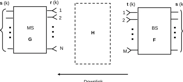
The model of joint Tx/Rx beamforming design for single user MIMO downlink system in flat-fading channel environment is illustrated in Figure 2-1. We consider a wireless communication system with M transmit and N receive antennas under the flat-fading environment. Thus, the flat-fading MIMO channel H can be represented by a channel matrix with dimension N×M. The input symbol streams are passed through the transmit beamforming F (pre-filter) which is optimized for a known channel and then the pre-filter output is transmitted into the flat-fading MIMO

channel. The received signal is processed by the receive beamforming G (post-filter). In this thesis, we will not consider coding and modulation design and only concentrate on transmit and receive beamforming design.

BS

…

s (k) t (k) M 1 2 r (k)

…

N 1 2 MS s (k)

…

…

Downlink H F G

For a MIMO channel without any delay-spread, the joint beamforming design system equation can be written as

Gn GHFs

sˆ= + (2.2.1-1) where H is the MIMO channel matrix described as above, sˆ is the B×1 received vector, and s is the B×1 transmitted vector. Note that

( )

(

M N

)

rank

B= H ≤min , (2.2.1-2) is the number of parallel transmitted data streams. F is the M× transmit B beamforming matrix, G is the B×N receive beamforming matrix and n is the

1 ×

N noise vector. The transmit beamforming adds a redundancy of M − across B space, because the number of input symbols is just B but produces M output symbols transmitted simultaneously through M transmit antennas. That results the

performance improvement due to the diversity gain. Besides, the receive beamforming removes the redundancy that be introduced by the transmit beamforming and results B output data for detection.

To derive the beamforming, we assume the following properties:

{ }

H = ; E

{ }

H = ; E

{ }

H =0;

E ss I nn R_nn sn (2.2.1-3) where the superscript H represents the conjugate transpose (Hermitian) operation. For simplicity of analysis, we assume that the transmitted signals are uncorrelated and normalized to unit power. B=rank

( )

H , the full-loaded case, the elements of MIMO channel matrix are uncorrelated with full rank. If B<rank

( )

H , under-loaded case, we can also apply it to our system. However the over-loaded case B>rank

( )

H is not possible for any practical system that transmits independent data streams more than rank of the MIMO channel H in order to have an acceptable performance.

2.2.2 OFDM-based Case

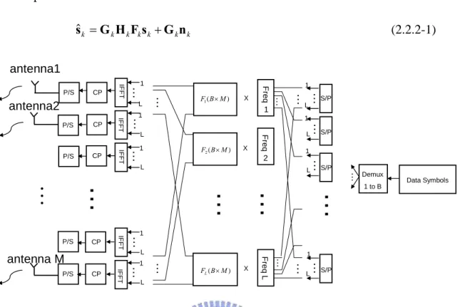
The OFDM technique which has attracted a lot of interest in the recent years as it can combat delay spread, easily deal with frequency selective channels and achieve the spectral efficiency described in section 1.2.1. Now, we apply the above MIMO system to the frequency selective channel with OFDM transmission, where the flat-fading conditions prevail on each subcarrier. The MIMO-OFDM system model in each subcarrier is similar to Figure 2-1. The difference is that the pro- and post-filter are processed at each subcarrier of OFDM. The MIMO-OFDM system equation has the similar form as the flat-fading case (2.2.1-1) and is shown as below where

subscript notation k of denotes the subcarrier index k k k k k k k G H Fs G n sˆ = + (2.2.2-1) Data Symbols Demux 1 to B 1 L … L … L … … 1 1 … … Fr e q 1 Freq L

…

Fr e q 2 …

…

L … IF F T L 1 1 … … … … L 1 L 1 L 1 IF F T IF F T IF F T IF F T CP CP CP CP CP P/S P/S P/S P/S P/S X X X

…

…… _{( )} 1B M F × ) ( 2B M F × ) (B M FL × S/P

…

S/P S/P S/P L … L 1 1 … L 1 L 1 antenna1 antenna2 antenna M

M

CP-1 CP-1 CP-1 CP-1 CP-1 S/P S/P S/P S/P S/P FF T FF T FFT FF T FF T L 1 L 1 L 1 L 1 L 1 … … … … … … …

…

) ( 1B N G × ) ( 2B N G × ) (B N GL × C1 CB

…

…

P/S

…

Data Symbols … … … … C2 antenna1 antenna2 antenna N

M

Note that, in MIMO-OFDM based system, the transmit beamforming is

Figure 2-2 Joint Tx/Rx beamforming processing at transmitter of a single user MIMO-OFDM system

performed in frequency domain, that is, before the OFDM modulation. And the receive beamforming should be also performed in frequency domain, that is, after OFDM demodulation. Figure 2-2 and Figure 2-3 illustrate the detail operations at transmitter (BS) and receiver (MS) respectively.

2.3 Joint Tx/Rx Beamforming Design for Single User Case

2.3.1 Problem Description

Now we will design transmit and receive beamforming matrices F and G to minimize the accumulative MSE in the flat-fading MIMO channel environment. However, as explained before, the flat-fading characteristic is preserved at each subcarrier of OFDM. Thus, we modify the above MIMO system and directly design

k

F and G for the MIMO-OFDM system. The MSE matrix at each subcarrier of _k

MIMO-OFDM system is defined as the covariance matrix of the error vector and showed as below:

(

)

(

)

{ }

H k k k k k k k F ,G MSE F ,G E e e E = = (2.3.1-1) where e is the symbol estimation errors and defined as _k e_k = ˆ

(

s_k−s_k

)

. Replacing the system equation (2.2.2-1) into (2.3.1-1), we obtain the MSE matrix as below:

(

)

{ }

{

(

)(

)

}

(

)

[

]

[

(

)

]

{

}

(

)(

)

{

}

(

)( )

{

}

( ) (

)

{

}

{

( )( )

H

}

k k k k k k k k H k H k k k k k k k H k k k k k k k k k k k k H k k k k k k k k k k k k k k H k k k k H k k k k k E E E E E E s s n G s F H G s s n G s F H G n G s F H G n G s F H G s n G s F H G s n G s F H G s s s s e e G , F E + + − + − + + = − + − + = − − = = E ˆ ˆ (2.3.1-2)

is fixed and known at the transmitter and the receiver The MSE matrix in equation (2.3.1-2) can be simplified as:

(

) (

)(

)

(

) (

)

H k k k k k k H k k k H k k k k k k k k k F H G F H G I G R G F H G F H G G , F E _nn − − + + = , (2.3.1-3)

Thus, the minimize MSE problem can be stated as follows:

{ }

(

(

)

)

(

k kH

)

Tk k k k k p trace E k k , 2 trace subject to min = = F F G , F E e ,G F _(2.3.1-4)

where p_T,k is the transmitted power constraint at k-th subcarrier. Note that the above equation (2.3.1-4) is based on the Frobenius norm:

{ }

{

( )

}

(

{

( )

H

}

)

k k H k k k E trace trace E E e 2 = e e = e e (2.2.1-5) After formulating the problem of the joint beamforming design for transmitter and receiver over flat-fading channel and frequency-selective channel (OFDM-based). In the next section, we will continue to derive two other methods which have the same solution as the above transmit and receive beamformer.

2.3.2 Optimum Transmit and Receive Beamformings

2.3.2.1 Lagrange Multiplier Method

First, we use the method of Lagrange duality and Karush-Kuhn-Tucker (KKT) conditions to solve the joint design problem in equation (2.3.1-8). We add the Lagrange multiplier μ_k to form the Lagrangian shown as below:

(

k k k

)

trace

(

E

{ }

k Hk

)

k

[

trace

(

k kH PTk

)

]

L μ ,F ,G = e e +μ FF − , (2.3.2.1-1)

(

)

[

(

)(

)

(

) (

)

]

k

[

(

k kH Tk

)

]

H k k k k k k H k k k H k k k k k k k k k P trace trace L , , , , − + − − + + = F F F H G F H G I G R G F H G F H G G F _nn μ μ (2.3.2.1-2)

The following KKT conditions are necessary and sufficient to solving the optimal transmit and receive beamforming F and _k G . _k F and _k G are optimal solutions _k if and only if there is a μ_k that together with F and _k G satisfy the conditions: _k

(

, ,

)

=0 ∇ L _{k k k} k F G F μ (2.3.2.1-3)

(

, ,

)

=0 ∇ L _{k k k} k F G G μ (2.3.2.1-4)

(

, ,

)

=0 ∇_μkL μ_k F_k G_k (2.3.2.1-5) From the equation (2.3.2.1-3) and (2.3.2.1-2), we can obtain

0 , = + − H k k k k H k H k H k k kFF H G H F R G H _nn (2.3.2.1-6) and from the equation (2.3.2.1-4) and (2.3.2.1-2), we can obtain

0 = + − H k k k k k k H k H k H k k kFF H G G H G H F H μ (2.3.2.1-7) To obtain above two equations, we have to use the fact:

(

)

(

∂ trace AXB

) ( )

/ ∂X =BA (2.3.2.1-8)

(

)

(

∂trace AXHB

)

/

( )

∂X =0 (2.3.2.1-9)

Now we are going to solve the two equations (2.3.2.1-6) and (2.3.2.1-7) to obtain the optimal transmit and receive beamformer. First of all, we define the SVD of following equation:

(

)

(

)

H k k k k k k k k H k V V S 0 0 S U U H R H _nn1, ~ ~ ⎟⎟ ~ ⎠ ⎞ ⎜⎜ ⎝ ⎛ = − (2.3.2.1-10)

and S is a diagonal matrix with B nonzero singular values with decreasing order.

k

S~ is a diagonal matrix with zero singular values; U~_k and V~_k are orthogonal matrices with dimensions M×

(

M −B

)

which form a basis of the null space of

k k H kR H H _nn1 , −

. Note that we have assume that the rank of H is B for simplicity. _k Applying the similar approaches used in [7], we can obtain the transmit and receive beamforming matrices with structures as follows:

k k k V ΦF F = (2.3.2.1-11) 1 , − = H _k k H k k ΦG U H Rnn G k (2.3.2.1-12) Where k F

Φ and Φ_Gk are diagonal matrices with nonnegative values and with dimension B× . Thus, the transmit and receive beamforming matrices diagonalize B the MIMO channel matrix into a set of eigen subchannels. We will explain the results in section 2.3.3. The diagonal matrices

k

F

Φ and

k

G

Φ in above two equations are

given by:

(

1₂ 1₂ 1

)

12 + − − − − = _{k k k} k S S Φ_F μ (2.3.2.1-13)

(

)

2 12 1 1 2 1 2 1 − + − − − = _{k k k k} k S S S Φ_G μ (2.3.2.1-14) The subscript notation + denoted that the negative elements of the diagonal matrices are replaced by zero and μ_k in the above two equations is chosen to satisfy the transmit power constraint and given by:

( )

1 , 2 1 2 1 − − + ⎟ ⎠ ⎞ ⎜ ⎝ ⎛ = k k T k k trace P trace S S μ (2.3.2.1-15)

Up to now, we have showed the Lagrange multiplier approach to derive transmit and receive beamforming matrices. In next section, we show another method to derive these beamforming matrices. These approaches are different, but the results are identity since both of them are looking for the optimal solutions.

2.3.2.2 Two Step Method

Recall that the minimized accumulative MSE problem is stated in (2.3.1-4) and the accumulative MSE matrix is given in equation (2.3.1-3). We now use the two-step derivation approach to design the system. In first step, we derive the optimal receive beamforming matrix G by assuming that the transmit beamforming matrix is fixed _k and then leave the difficult part which is to derive the transmit beamforming matrix

k

F to next step.

The optimal receive beamforming solution G_{k ,opt} that minimizes the MSE matrix is the same as the Wiener solution which is known to minimize the

(

)

(

MSE _{k k}

)

trace F ,G and is given by the following equation

( )

(

G

)

0

G =

∇ trace MSE _k

k (2.3.2.2-1)

And then the optimal solution G_{k ,opt} can be obtained as below:

(

)

1 , , − + = H _k k H k k k k k opt k F H H F F H Rnn G (2.3.2.2-2) The optimal receive beamforming is exactly the Wiener filter solution. Replacing the optimal receive matrix G_{k ,opt} into the MSE matrix, we obtain the following concentrated error matrix:

(

)

(

)

(

₁

)

1 , 1 , , − − − + = + − = k k H k H k k k k H k H k k k H k H k opt k k k H R H F I F H R H F F H H F I G , F E nn nn (2.3.2.2-3)

Thus, the joint beamforming design problem is simplified to the design of the transmit beamforming with the receive beamforming matrix given by Wiener solution (2.3.2.2-2). Note that, without any constraint, the minimization of (2.3.2.2-3) will lead to the trivial solution of increasing to infinity of the norm of F . Thus, the solution of _k the optimization problem with transmit power as a constraint:

(

)

(

)

(

k kH

)

Tk opt k k k p trace trace k k , , subject to min = F F G , F E G , F (2.3.2.2-4)

is given by F_k =V_kΦ_Fk , where Φ is a _Fk B× diagonal matrix with the following B elements 2 1 , 2 1 , 1 2 1 , 1 1 , , , 1 + − = − = − ⎟⎟ ⎟ ⎟ ⎟ ⎠ ⎞ ⎜⎜ ⎜ ⎜ ⎜ ⎝ ⎛ − + =

∑

∑

k ii k ii B j jjk B j k jj k T k ii P λ λ λ λ φ (2.3.2.2-5)

where λ_k denotes the singular values of the matrix S . The above equation is _k actually equivalent to the elements of equation (2.3.2.1-13) which is the matrix form. If we replace the transmit beamforming into the optimal receive beamforming matrix derived in first step, we can obtain the same optimal receive solution given in section 2.3.2.1.

2.3.3 Equivalent Decomposition of MIMO-OFDM system

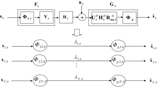
mutually cross-coupled MIMO transmission system into a set of parallel eigen subchannels (also termed channel eigenmodes) system. From the results of previous section, the matrix model of MIMO-OFDM system at k-th subcarrier similar to flat-fading case can be illustrated in Figure 2-4.

k , f

Φ

V

_k H_k 1 nn

R

H

U

− k H k H k ,

Φ

g

+

Downlink k

F

n

k

G

_k k

sˆ

k

s

Mathematically, the product of optimal beamforming matrices F_{k ,opt} and G_{k ,opt} in equation (2.3.2.1-11) and (2.3.2.1-12) and the channel matrix H becomes: _k

k k k k H k H k opt k k opt k H F ΦG U H Rnn H VΦF G k 1 , , , − = (2.3.3-1) Using the SVD in equation (2.3.2.1-10), it can be rewritten as:

k k k k H k k k H k opt k k opt k H F ΦG U U S V VΦF ΦG S ΦF G , , = _k = _k (2.3.3-2) Since k G Φ ,S and _k k F

Φ are all diagonal matrices, the MIMO channel are

decoupled into parallel eigen subcarriers. Figure 2-5 illustrates the equivalent MIMO-OFDM system at k-th subcarrier.

M

k f,

Φ

_1, k f,

Φ

_2, k f,N

Φ

_, k , f Φ V_k H_k 1 nn

R

H

U

H − _k k H k ,

Φ

g

+

k F nk Gk k sˆ k s k , 1 s k , 2 s k N , s k g,

Φ

_1, k g,

Φ

_2, k g,N

Φ

_, k , 1 ˆ s k , 2 ˆ s k N , ˆ s k , 1

λ

k , 2

λ

k N ,

λ

The major interest of the diagonalized structure is that all the matrix equations can be substituted with scalar ones with the consequent great simplification and only the symbol by symbol detection need to be performed.

2.4 Conclusions

In this chapter, we have shown the system model for flat-fading channel environment and extend to OFDM-based system which can combat the frequency selective channel and achieve the spectral efficiency. Each subcarrier of MIMO-OFDM based system can be treated as flat-fading case and solved by the same ways. We have also developed two forms of joint MMSE transmitter-receiver beamforming: the Lagrangian and the two-step methods. Both approaches result in the same close-form solution.

The joint design problem shows that the optimal beamforming matrices F_{k ,opt}

and G_{k ,opt} in equation (2.3.2.1-11) and (2.3.2.1-12) cascaded with the channel matrix

k

H in between will result in a diagonal matrix. That is, the original mutually

cross-coupled MIMO transmission system is decoupled into a set of parallel eigen subchannels system. It means that the matrix equations can be simplified to scalar ones so that we can perform symbol by symbol detection similar to a set of parallel SISO systems. This joint design approach makes the number of antennas, the size of the coding block, and the transmit power become scalable.

---

Chapter 3

Joint Tx/Rx MMSE Beamforming Design for

Multi-user MIMO-OFDM SDMA Downlink

System with Perfect CSI

---

In this chapter, we extend the single user joint Tx/Rx beamforming design to the multi-user case so that we can achieve the multiple access via the space domain the so called spatial-division multiple access (SDMA) [15] [18]. Compare to the conventional frequency-division multiple access (FDMA) and time-division multiple access (TDMA), the SDMA can conduct multi-user transmission at the same time and frequency. That is, we can reuse the frequency bandwidth. However, the multi-user interference (MUI) can potentially cause performance degradation. The technique of null-spacing [18] is proposed to handle the MUI problem.

3.1

Introduction

Different from most of the SDMA systems which assume a single antenna equipped at mobiles, the MIMO system we consider is the system with multiple

antennas used at both transmitter and receiver. We will further extend the MIMO SDMA system to MIMO-OFDM SDMA system by the concepts mentioned in chapter 2. In the multiple access system, the MUI is a major problem which causes significant performance loss. A way of solving this problem is to use the null-space constraint to decouple the multi-user MIMO SDMA joint design problem into several single user problems which have been described in previous section, where each problem only depends on each single user MIMO channel. In other words, the product of the MIMO channel and the null-space matrix at transmit side results in a block-diagonal matrix, which means the MUI between each user is completely removed. Thus, each user terminal only has to deal with its own inter-stream interference.

In this chapter, we first model the single carrier flat-fading MIMO SDMA system which combines the joint Tx/Rx beamforming design with the null-space technique. Then we extend such system to MIMO-OFDM SDMA case which preserves the flat-fading property at each subcarrier. Thus, the beamforming and null-space matrices have to be designed based at each subcarrier. That is, we have to perform the pre-filter with the null-space constraint before OFDM modulation at the transmitter and at the receiver. The post-filter is also performed after OFDM demodulation. The null-space matrix design technique will be introduced in section 3.3.1. Thereafter, we will introduce the combination of the joint Tx/Rx beamforming and the null-space constraint to deal with the multi-user MIMO-OFDM SDMA downlink system.

3.2

Joint Tx/Rx Beamforming MIMO SDMA System Models

3.2.1 MIMO SDMA under Single Carrier Flat-fading Channel

Figure 3-1 illustrates a multi-user MIMO SDMA downlink system under single carrier flat-fading channel. We consider the transmit side (BS) equipped with M antennas simultaneously communicates with U user terminals (mobile station or MS). Each user terminal has N receiver antennas. The BS transmits several data u symbol streams towards the U user terminals simultaneously. C data streams are 1 transmitted towards user terminal 1, C data streams are transmitted towards user 2 terminal 2, and so on.

H

…

_BS

…

C1 CU … … 1 M 2 s1_(k) sU_(k) t(k)

…

MS-1 MS-U

…

…

1 N1 1 NU r1_(k) rU_(k)

…

…

C1 CU s1_(k) sU_(k) Downlink

If we do nothing at BS, each user terminal will receive the mixture of all data streams and needs to recover its own streams. Note that the receiver antennas N of u each user terminal is greater or equal to the number of data streams C in order to u make sure an acceptable performance.

The joint Tx/Rx beamforming design combined with null-space matrix can be

depicted in Figure 3-2. 1 W _WU 1 H U H

…

_…

∑

= × U u u D M 1 M Nu_×

∑

1 F U F 1 G U G 1 1 _C D × U U _C D × 1 1 _R C × U U _N C ×

…

_…

C1 CU C1 CU 1 1 N 1 U N 1 M

…

…

…

…

…

O

0 0 0 0 0 0 G 1 G

O

0 0 0 0 0 0 F 2 G U G 1 F 2 F U F

∑

∑

_Cu× _Nu

∑

∑

_Du× _Cu

M M

K

K

K M

M M

K

K

K

M

O

0 0 0 0 0 0 1 1 _D N × U U _D N ×

K

_K

K

M M

M

× ×

∑

∑

_Nu× _Du 3.2.2 MIMO-OFDM SDMA

By using the OFDM technology, the transmit beamforming and null-space matrix is designed based on each subcarrier and performed before OFDM modulation at the transmit side. At each user terminal, the receive beamforming is also designed based on each subcarrier and performed after OFDM demodulation. And at each subcarrier, the flat-fading conditions prevail and can be treated as above single carrier flat-fading MIMO system shown in Figure 3-2.

3.3

Joint Tx/Rx Beamforming Design for Multi-user Case

3.3.1 Null-space Constraint Design

Now we introduce the design of the null-space matrix which block-diagonalizes

the MIMO channel. The following design is based on MIMO-OFDM system where the subscript notation k denotes the subcarrier index. In order to remove the MUI between each user, a null-space matrix denoted by W is designed that the product _k of the MIMO channel matrix and the null-space matrix H_kW_k at k-th subcarrier results a block-diagonal matrix with u-th block in the diagonal which is u-th user’s data streams. That is the MUI is completely eliminated and leaves only each user’s inter-stream interference which can be deal with by each user’s processing.

) ( R T H

∑

u×

…

) ( 2 2 _{N M} H × ) ( 1 1 _{N M} H × ) (N M HU U _× ) ( N M H

∑

u _×

First of all, the multi-user MIMO channel matrix H at k-th subcarrier can be _k viewed as a vertical concatenation of U MIMO subchannels matrix H which u_k means the BS to u-th user’s MIMO subchannel at k-th subcarrier and with dimension

M Nu_×

. We illustrate the whole multi-user MIMO channel by Figure 3-3.

In order to block-diagonalize the whole MIMO channel matrix H , we have to _k design the null-space matrix W with horizontal concatenation of _k U sub-matrices