線上購物零售業之消費者退貨影響因素分析
73
0
0
全文
(2) 線上購物零售業之消費者退貨影響因素分析. 學生:孫馨璍. 指導教授:馮正民 教授 黃昱凱 教授. 國立交通大學交通運輸研究所碩士班 摘. 要. 網際網路的代表著一新興市場,電子商務成為重新整合供應者與消費者關 係的新商業模式。資策會預期2008年臺灣B2C市場規模可達1385億,相較於去年 度的市場規模有38%的成長。由此可見,線上購物的規模與成長不容小覷。然而, 隨著市場的成熟,退貨也逐漸成為線上購物零售商所需克服的議題之ㄧ。過去的 文獻探討到退貨議題,往往集中在供應商與零售商間,但隨著線上購物的興盛, 零售商與終端消費者間的退貨議題,逐漸被受重視。 本研究擬針對線上購物之交易,利用實證資料以決策樹分類模型判別交易 是否退貨,藉以了解何判別變數影響顧客之退貨傾向。判別變數分為三大類別, 分別是顧客屬性變數、商品變數以及服務變數。 研究結果發現,變數中-商品種類、價格與配送天數能夠較有效地判別消 費者退貨傾向的高低,最後,針對決策樹所歸納出的規則與變數範圍,研擬對應 策略以作為網站管理者控制線上購物退貨之參考。. 關鍵字:線上購物零售業、退貨傾向、決策樹分類器.
(3) An Analysis of the Factors Affecting Consumers’ Propensity to Return in E-Retailing. Student:Xin-Hua Sun. Advisors:Prof. Cheng-Min Feng Prof. Yu-Kai Huang. Institute of Traffic and Transportation National Chiao Tung University. ABSTRACT The internet represents a growing and huge market. The development of e-commerce is an efficient business model which enables new relationship between consumers and suppliers. In particular, the B2C market in Taiwan is expected to reach NT $138.5 billion with 38% increase in 2008. The E-retailing is obviously becoming a noticeable market. However, as the market grows and matures, “return” becomes one of the challenges for E-tailers. In the past, most of the literature on return issues focused on the wholesaler-retailer relationship. Recently, due to the advent of Internet-based retailing within the past decade, attention is shifting to the issue of returns in the retailer-consumer relationship. In this study, we use empirical data and conduct a Decision Tree model to analyze the critical variables revealing the customer return propensity. There are 3 dimensions of variables in our data set- customer demographic variables, merchandise variables and service variables. We find that three variables- category, price and delivery days could be used to distinguishing customer return propensity more effectively. In accordance with these variables, we propose some strategies for website managers to control returns in E-retailing.. Keywords: E-retailing, Return Propensity, Decision Tree.
(4) 誌. 謝. 從第一次為北門的眉宇所驚豔,而今倏忽兩年過去,即將踏出北交的我們 也將揚首起步,朝向未來邁進。 在北交的這段期間,老師們的教導以及對論文的指正與建議;馮老師、昱 凱學長在論文指導的費心,和對於職涯上的經驗分享;洪姐、柳姐、何姐不厭 其煩地幫忙處理生活瑣事;博班學長姐在學術與就業的指引,謝謝你們過去的 提攜與奉獻。 ITT97 同學、ITT98 學弟妹,謝謝你們為研究生生活帶來的刺激,有這樣 一群同齡的朋友,共同分享撰寫論文過程中的苦與樂,一起在研究的過程中激 發對科學探討的興趣,一起在閒暇時出遊、開 Party,使得兩年的生活過得更加 充實、快樂。 謝謝所有分擔了我的責任和激勵我成長的人,感謝賦予我生命與思辨能力 的爸媽,我的成就歸功於你們不曾間斷的付出。. 2008 年 6 月於台北交研所.
(5) Table of Contents CHAPTER1. INTRODUCTION...........................................................1. 1.1 Research Background and Motivation..........................................................1 1.2 Research Objectives......................................................................................2 1.3 Research Scope .............................................................................................3 1.4 Research Procedures .....................................................................................3. CHAPTER2. LITERATUREE REVIEW ............................................5. 2.1 E-retailing .....................................................................................................5 2.2 Return Issues in E-retailing.........................................................................10 2.3 Data Mining ................................................................................................12 2.4 Summary .....................................................................................................14. CHAPTER3. METHODOLOGY........................................................16. 3.1 Classification Model ...................................................................................16 3.2 Decision Tree Induction..............................................................................17 3.3 Research Framework ..................................................................................19. CHAPTER4. EMPIRICAL DATA ......................................................21. 4.1 Case Introduction ........................................................................................21 4.2 Data Collection ...........................................................................................24 4.3 Data Preprocessing......................................................................................26 4.3 Variable Explanation...................................................................................27 4.4 Data Analysis ..............................................................................................29. CHAPTER5. RESULTS AND ANALYSIS.......................................39. 5.1 Setup and Sampling ....................................................................................39 5.2 Model Development....................................................................................40 5.3 Results Discussion ......................................................................................47 5.4 Developing Strategy....................................................................................52. CHAPTER6. CONCLUSION AND SUGGESTION.........................57. 6.1 Conclusion ..................................................................................................57 6.2 Limitations and Suggestions .......................................................................58. REFERENCE..........................................................................................59 APPENDIX..............................................................................................62. I.
(6) List of Figures FIGURE 1.1 FIGURE 2.1. FIGURE 2.2. FIGURE 3.1 FIGURE 3.2 FIGURE 3.3 FIGURE 4.1 FIGURE 4.2 FIGURE 4.4 FIGURE 5.1 FIGURE 5.2 FIGURE 5.3 FIGURE 5.4. RESEARCH PROCEDURE ..............................................................................4 INTEGRATED PRODUCT RETURNS SYSTEM............................................... 11 STRUCTURAL EQUATION MODEL .............................................................12 GENERAL APPROACH FOR BUILDING A CLASSIFICATION MODEL ..............16 AN EXAMPLE OF DECISION TREE ..............................................................18 ANALYSIS PROCEDURE OF DECISION TREE ...............................................20 ORDER PROCEDURE OF ONLINE SHOPPING ...............................................22 RETURN PROCEDURE OF ONLINE SHOPPING .............................................23 DISTRIBUTION OF AGE DATA ....................................................................37 DATA SAMPLING .......................................................................................40 RETURN PROPENSITY WITH PRICE.............................................................53 RETURN PROPENSITY WITH AVERAGE DELIVERY DAYS ............................54. DELIVERY SCHEDULING ON WORK DAYS .................................................54 FIGURE 5.5 DELIVERY SCHEDULING ON WEEKEND .....................................................55 FIGURE 5.6 ADJUSTED DELIVERY SCHEDULING ON WEEKEND ....................................55 FIGURE 5.7 TRANSACTION FREQUENCY AND AVERAGE RETURN FREQUENCY .............56. II.
(7) List of Tables TABLE 2.1 INTERNET BUSINESS MODEL ........................................................................5 TABLE 2.2 RE-THINKING THE E-RETAILING PROCESS ....................................................9 TABLE 4.1 DESCRIPTION OF ORIGINAL DATA ...............................................................25 TABLE 4.2 DESCRIPTION OF INPUT VARIABLES ............................................................28 TABLE 4.3 TARGET VARIABLE .....................................................................................29 TABLE 4.4 GENDER / RETURN CROSS TABULATION .....................................................29 TABLE 4.5 LOCATION / RETURN CROSS TABULATION ..................................................30 TABLE 4.6 MERCHANDISE CATEGORY / RETURN CROSS TABULATION .........................32 TABLE 4.7 PAYMENT / RETURN CROSS TABULATION....................................................34 TABLE 4.8 DELIVERY APPROACH / RETURN CROSS TABULATION ................................34 TABLE 4.9 CARRIAGE / RETURN CROSS TABULATION ..................................................35 TABLE 4.10 ACTUAL DELIVERY DAYS / RETURN CROSS TABULATION.........................35 TABLE 4.11 AVERAGE DELIVERY DAYS / RETURN CROSS TABULATION .......................36 TABLE 5.1 TABLE 5.2 TABLE 5.3 TABLE 5.4 TABLE 5.5 TABLE 5.6 TABLE 5.7 TABLE 5.8. INFORMATION OF DECISION TREE SETTING ................................................39 GENERAL INFORMATION OF DECISION TREES .............................................40 SELECTED RULES OF DECISION TREE-FEMALE CUSTOMERS ......................41 SELECTED RULES OF DECISION TREE- MALE CUSTOMERS .........................43 SELECTED RULES OF DECISION TREE- LOW FREQUENCY CUSTOMERS .......44 SELECTED RULES OF DECISION TREE- HIGH FREQUENCY CUSTOMERS ......45 SELECTED RULES OF DECISION TREE-FEMALE MERCHANDISE ..................47 GENERAL INFORMATION OF DECISION TREES .............................................52. III.
(8) CHAPTER1. INTRODUCTION. 1.1 Research Background and Motivation The internet represents a growing and huge market. The development of e-commerce is an efficient business model enables new relationship between consumers and suppliers. Consumers can surf on the internet, browse the information, and compare prices of diversified merchandise. For suppliers, internet represented a new business channel for suppliers and consumers. An October 2007 report established by MIC1 in Taiwan, the online shopping market is anticipated to be NT $185.5 billion in 2007. Furthermore, the expected growth rate in 2008 will be 36% and the total amount will be NT $250 billion in 2008. In Particular, the B2C market is expected to reach NT $108 billion with 31% increase. In 2008, the growth rate of B2C market will be 38% and the total amount of business volume will be NT $138.5 billion. The online shopping is obviously becoming a noticeable market. As this percentage continues to increase, so does the need to understand why and how users choose to adopt it instead of offline channel, which helps researchers and e-commerce providers to get a better understanding of the future adoption of E-commerce. (Sungjoo Lee, 2007) Some problems in E-retailing include an unproven financial model; high merchandise return rates; establishing customer trust; distribution costs; bounded rationality and the different cognitive process between fun and routine purchases (Stern, 1999). While the E-retailing market developing continually and maturely. The number of retailer increases and the competition among retailers turn to be severe as well. The furious competition is not only in price of various merchandises but also in service of specific website. Some E-tailers use loose return policy as a symbol of service upgrade as well as a marketing approach to broaden customer base. Much of the literature on return issues focused on the wholesaler-retailer relationship (Kandel, 1996; Padmanabhan & Png, 1997), recent attention is shifting to the issue of returns in the retailer-consumer relationship. This change results from the advent of Internet-based retailing within the past decade. (Mollenkopf et al., 2007). 1. MIC, Market Intelligence Center was established in 1987, which is a division of Taiwan's Institute for Information Industry 1.
(9) To better understand the crucial factors of returns and effectively reduce the return rate in E-retailing, this study aims to use empirical data and data mining analysis to understand how the consumer characteristics, merchandise dimension and service affect returns in E-retailing market.. 1.2 Research Objectives There are several objectives of this study defined bellow: 1.. Review the significant case of E-retailing in Taiwan and the return process of internet shopping. Explaination: To fully understand the process of return operation in e-retailing, we review a major website in Taiwan which provides a virtual channel for retailers.. 2.. Identify the critical factors that related to returns in transaction process. Empirical data and data mining technology applied. Explaination: After reviewing the significant case and literature, we will select some predicted variables as observed variables. To continue, we will use Decision Tree (One of the classification technique of Data Mining) to distinguish whether an order was returned or not, meanwhile, to indicate the critical variables relating to return propensity in E-retailing market.. 3.. Apply return knowledge to propose suggestion on developing strategies to the website managers and retailers in E-retailing market. Explaination: The result of decision tree will demonstrate some important rules of return propensity. This study will finally try to provide available strategies based on the outcome of data mining.. This study will provide a dominant influence in understanding consumers’ propensity of return and. In the final, it will give E-retailing managers a comprehensive insight while developing return strategies for targeted customers.. 2.
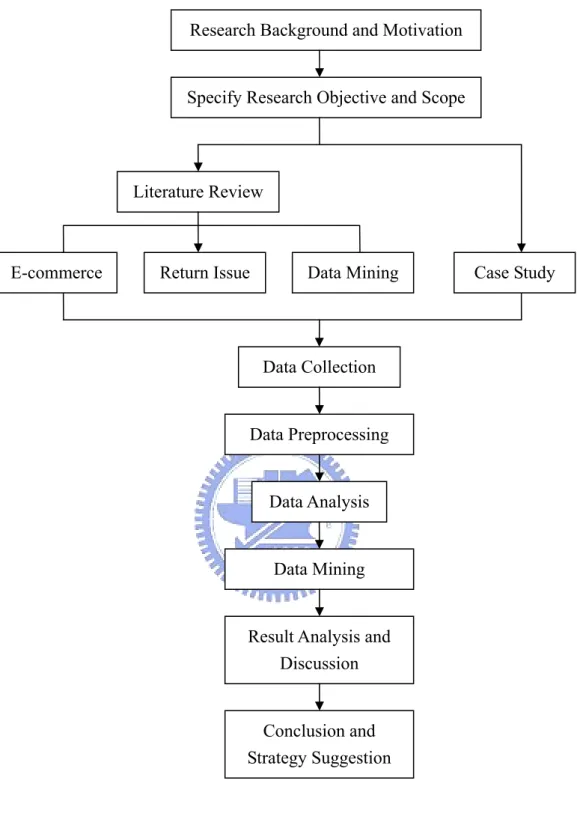
(10) 1.3. Research Scope. This study will review the impact of return upon E-commerce. Particularly we will focus on B2C business model, which concentrates on the business to end-consumer view of e-commerce, often termed E-retailing. In the case study of empirical analysis, the business part is separated to two participants. One is the website operator and the other one is the retailers solicited by the website operator. The website operator is responsible for soliciting from diverse merchandise suppliers and unifying the information flow and payment flow. The website operator is namely the intermediary between retailers and consumers. On the other hand, the retailers are responsible for deciding the marketing strategies and inventory flow. Consumers search information, order items and pay the bill via the website platform. And then, retailers pick up the items to be delivered according to the orders. Only physical merchandise will be discussed in this study while financial and digital merchandise will be excluded. Exchange service will be included in this study. However, it is transformed to return the undesirable items and purchase a new one.. 1.4 Research Procedures In Chapter1, this study defines research objectives while explaining an outlook of this issue. The remaining of this study is organized as follows: Chapter2 describes some background and reviews on previous related literatures. Chapter3 introduces the research methodology and the impending research procedure. In Chapter 4, we will introduce the overview of our case and data resource. Statistical description of each variable will also be involved in this chapter. Chapter 5 presents the output of decision tree and provides some discussion of our results. This study concludes with a summary of its contributions and directions for future research in Chapter 6.. 3.
(11) Research Background and Motivation. Specify Research Objective and Scope. Literature Review. E-commerce. Return Issue. Data Mining. Data Collection. Data Preprocessing. Data Analysis. Data Mining. Result Analysis and Discussion. Conclusion and Strategy Suggestion. Figure 1.1 Research Procedure. 4. Case Study.
(12) CHAPTER2. LITERATUREE REVIEW. 2.1 E-retailing 2.1.1. The definition of E-retailing. The Internet currently plays an important role as a business medium. People use the Internet as a business medium, so-called electronic commerce (e-commerce) (Eastin, 2002). More precisely explanation could refer to the definition adopt by Grandon and Pearson (2004): the process of buying and selling products or services using electronic data transmission via the Internet and the www. Based on two classification schemes- Seller and Buyer, e-commerce can be placed into four categories. There are: B2B, B2C, C2B, and C2C business model. This study will focus on business-to-consumer model which concentrates on the business to end-consumer view of e-commerce, often termed e-retailing. Table 2.1. Internet Business Model. Buyer Seller. Business Consumer. Business. B2B. B2C. Consumer. C2B. C2C. Source: Kricjnamurthy, 2003. Defined by Kricjnamurthy (2003), business models in the B2C sector can be broadly classified as 5 groups as below: 1.. Direct sellers Direct sellers make money by selling products or services to consumers. Their primary source of income is the margin on each transaction. There are two types of direct sellers- E-tailers and manufacturers. E-tailers, such as Amazon.com, collect orders from consumers and either directly ship the products or pass the order on to wholesalers or manufacturers for delivery. Manufacturers that sell directly are using the power of the Internet to reach customers directly. A prime example of this is Dell.com gaining market power by establishing direct customer relationships. 5.
(13) 2.. Intermediaries Online intermediaries are the largest number of B2C companies today. These companies facilitate transactions between buyers and sellers and receive a percentage of the value of each transaction. B2C intermediaries are of two types- brokers and infomediaries. Brokers facilitate transactions between buyers and sellers. Infomediaries act as a filter between companies and consumers. Individuals provide the infomediary with personal information and, in turn, receive targeted ads and offers. Companies can buy aggregated market research reports and target individuals based on data held private by the infomediary. Brokers make money by charging a fee on each transaction; while informediaries make money by selling market reports and helping advertisers target their ads. One example of broker is virtual mall- a company that helps consumers to buy from a variety of stores. The company makes money on each transaction (e.g., Yahoo! Stores, Rakuten). Broker is also the role of the case introduced later in this study.. 3.. Advertising-Based Business These businesses have ad inventory on their site and sell it to interested parties.. 4.. Community-Based Model Community-based models allow users worldwide to interact with one another on the basis of interest areas. These businesses make money by accumulating loyal users and then targeting them with advertising.. 5.. Fee-Based Model This type of business charges viewers a subscription fee to view its content.. 2.1.2. Characteristic of E-retailing. Shopping online is more complex than traditional shopping, where consumers select, purchase and then leave a store with their items. The online shopping process involves finding an appropriate site and then navigating that site to select and make purchases. The next part of the process involves waiting for fulfillment, checking the order when it arrives, and returning it if there is a problem (Boston Consulting Group, 1998). 6.
(14) Reynolds (1997) identified four major challenges for e-retailing.: the transferability of retail brands; the appropriateness and availability of distribution networks; the market share practicalities of extending market reach; and supplier relationships. He concluded ‘‘a truly profitable, transactional presence on the Internet appears somewhat more problematic than many of its proponents would have retailers believe’’ in 2000. Wood (2001) pointed when consumers shop by catalog or internet, their physical remoteness from product creates two key differences from in-store shopping. First, direct examination of the product alternatives is precluded, and therefore the quality of information about sensory product attributes may be inferior. Second, for non-digital products, customers cannot simply take their purchases home; they must wait for delivery to gather the kind of experiential information that is present during in-store purchases. Both characteristics raise the level of risk to the consumer. Lee and Tan (2003) integrated extant literature on retailing and consumer choice to develop an economic model of consumer choice in which a consumer self-selects between online and in-store shopping. Two important factors impacting consumer choice between online versus in-store shopping are identified: (1) the retail context utility and (2) the consumers’ perceived product and service risks. The model developed by Lee and Tan (2003) postulated that consumers derive utility from the shopping experience and are more likely to shop online for products/services that are low in purchase risks. Consumers are also more likely to shop online for products with well-known brands than lesser-known ones. However, they are less likely to shop online from lesser-known retailers who carry well-known brands than from reputable retailers, even if the latter carry lesser-known brands. The result confirmed that most consumers still value the physical aspects of a shopping experience. It also shows that consumers’ perceived product risk may not necessarily be higher for the online shopping context. However, consumers do perceive service risk to be higher in the online shopping context. The close correlation between risk aversion and Internet shopping tendency shown suggested that traditional retailers and entrepreneurial startups who are contemplating venturing into online retailing should focus on the less risk-averse consumers as their initial target segment. The result also implies that traditional retailers could use the appropriate risk relievers to lower the perceived risk of the more risk-averse consumers. In the end of this study, the authors suggested well-established traditional 7.
(15) retailers could use their known reputation and/or well-known brands as risk relievers to reduce the risk aversion of online consumers. New startups in electronic retailing are disadvantaged by their lack of an established reputation. Entrepreneurial start-ups in electronic retailing can reduce consumers’ perceived risk of purchase by carrying only well-known brands. Burt and Sparks (2003) considered the retail process as five directions: comprising the sourcing of products; stockholding, inventory and store merchandising; the marketing effort including branding; customer selection, picking and payment; and distribution of items by or to the consumer. (See Table 2.2) They pointed that buyers and suppliers that have previously had trouble reaching each other can connect in E-retailing. Suppliers can gain access to more buyers. Buyers can participate easily and view items from multiple suppliers. The electronic interface should lower transaction costs for both buyer and seller, and this transparency will likely drive down prices as well. E-retailing provides a 24 hrs shopping opportunity and in theory widens the “store” catchment area from the local to national or global level. Thus the traditional retail boundaries of “store reach” are changed both temporally and geographically. Further observation, in most sectors the logistics process and associated activities have moved towards fewer large consolidated drops whether to a centralized depot or store. The in-built inefficiencies in terms of cost and service levels of a large number of direct deliveries (to store) are recognized. However, e-retailing would appear to reverse or add to this process, requiring a large number of small drops (to the home). In reality these journeys currently take place but the scheduling and cost of this activity is borne by the customer. In an e-retailing system, the management of this process (and possibly the cost) will now be passed on to the retailer.. 8.
(16) Table 2.2 Re-thinking the E-retailing Process Aspects Sourcing of products Stockholding, inventory and store merchandising. Activity/process. Costs. Unchanged, though retailer dominance of supply chains possibly enhanced. Online activity, Information and not product more important, more QR and JIT type activity. Probably unchanged, though Potential to reduce costs of in some categories potential to stockholding through less transfer stock to supplier stock, but to increase costs of transport. Some online replenishment benefits and possible stock reduction. Brand ownership become More spend on the brand, but more critical including retailer unclear about the returns brands, but also key manufacturer brands (of which there will be fewer). Reduced efficiency for retailers, but less clear for manufacturers, potential for gains from loyal customers. Consumers taking ownership but retailers left to do the process, e.g. picking and delivery. Retailers may see costs rise. Reduced retailer efficiency. Currently done by consumers but moving to retailer. Costs will be incurred, for some retailers the consumer may be persuaded to pay. Reduced efficiency for retailers. Menus and scripts will help customers, possibilities of Automated replenishment for some. Distribution of Outsourced and/or goods, by, or to consolidated the customer Source: Burt and Sparks (2003).. Potentially reduced for all parties. Efficiency. Electronic linkages, online relationships. Corporate branding may The marketing become more important, effort including multi-channel retailing will branding grow, clearer view of customer loyalty Customer selection, picking and payment. Ownership. Efficiency gains, arguably to all parties.
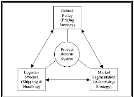
(17) 2.2 Return Issues in E-retailing Yalabik et al. (2005) focused on the system-design level of return management system. They identified three components of an integrated product returns system that can improve a company’s bottom line. The first component is the refund policy. In any purchase, even if the customer is well informed about the product, there is a possibility that after taking the product home the customer might realize that the product is not exactly what was expected. The customer obviously has some needs and is seeking fulfillment of those needs by buying the product. However, if the product turns out not to be what the customer thought it to be prior to the purchase, then those needs are not fully satisfied and the value of the product is reduced in the eyes of this customer. The customer, aware of this risk from the beginning, will be reluctant to go ahead with the purchase unless there is some protection mechanism. A refund policy provides such protection by allowing a customer to spend some time with the product before making a final decision. As a result, a refund policy decreases a customer’s risk associated with making a purchase, and thereby increases the total demand for the product. The second component is the logistics process. When a return occurs, both the retailer and the customer experience costs. For the customer, there is the transaction cost associated with returning a product (e.g., the expense and hassle of shipping) and for the retailer there is the handling cost associated with processing the return (e.g., the cost of repackaging). Thus, an efficient logistics process could result in either or both of two effects: Like a refund policy, it could increase total demand by reducing the customer’s cost associated with making a purchase; or it could increase the average profit margin by reducing direct costs. The third component is the marketing initiative to sharpen market segmentation. Recall that, in any purchase, there is some probability that the product will not match what a given customer thought it to be prior to the purchase. However, the greater the a priori information content of the product’s characteristics, the better segmented the market will become, and thus, the higher the probability that a given purchase will result in a match between the product’s properties and the customer’s needs. Thus, an effective marketing initiative could result in an increased average number of matches per sale..
(18) Figure 2.1. Integrated Product Returns System. Source: Yalabik et al. 2005 Mollenkopf et al. (2007) provided evidence of the impact of the returns management system upon customer loyalty intentions by structural equation model. They suggested that when a customer initiates a return, this in effect presents a service recovery opportunity for the Internet retailer. They focused attention on the return service aspect of an Internet retailer’s relationship with its customers. Specifically, Mollenkopf et al. proposed that three variables directly and positively influence loyalty intentions: perceived value of the returns offering, return satisfaction, and previous service experience. Perceived value of the returns offering measures the customer’s perception of the entire returns management system, including both policy and process issues. The return satisfaction construct focuses more narrowly on the customer’s experience with a specific return transaction. Three important results were discussed. First, return processes that require high levels of customer effort can have a severely negative impact on a customer’s satisfaction with the return transaction. Second, the results demonstrated not only does previous service experience have a strong direct effect upon loyalty intentions, but it also indirectly affects customers’ loyalty intentions through their satisfaction with, and the value they perceive from, the returns offerings. Third, managers should evaluate their firm’s service recovery quality in terms of recovery responsiveness, compensation, and contact. The ability to respond promptly and appropriately to a customer’s return situation, the manner in which customers are compensated for problems, and the accessibility of knowledgeable customer service representatives 11.
(19) (live or through online chats) during the return process all have a strong influence on a customer’s perceived value of the returns offering, which in turn affects the customer’s loyalty intentions.. Figure 2.2. Structural Equation Model Source: Mollenkopf et al. (2007). 2.3 Data Mining 2.3.1. Data Mining in E-commerce. Data mining techniques are applied to solving recommendation problems in e-commerce in most cases. Recommendation systems track past actions of a group of customers to make a recommendation to individual members of the group. Web usage mining is the process of applying data mining techniques to the discovery of behavior patterns based on Web data. With the advance of e-commerce, the more individualized data collection generated by systems provides the opportunity for more refined segmentation and targeting of activities. The importance of Web usage mining is growing larger than before. The overall process of Web usage mining is generally divided into two main tasks: data preparation and pattern discovery. The data preparation tasks build a server session file where each session is a sequence of requests of different types made by a single user during a single visit to a site. (Kim et 12.
(20) al., 2002) Kim et al. (2002) focused on the recommendation problem of helping selective customers find which products they would like to purchase by suggesting a list of top-N recommended products for each of them at a specific time. The suggested procedure is based on Web usage mining, product taxonomy, association rule mining, and decision tree induction. This personalized recommendation procedure can get further recommendation effectiveness when applied to Internet shopping malls. Lee et al. (2007) identified some characteristics of services which encourage customers to buy online and to develop a prediction model for success based on customer recognitions of service offerings in e-commerce. A review of Decision Tree model reveals that purchasing frequency and price are key factors for online services by being selected as decision criteria at the first layer. These factors are in fact important attributes of the general products in e-commerce. Besides the above two factors, labor intensity, criticality and contact time representing the service characteristics are also factors that are selected as decision criteria at the second layer. The findings provide a guide for those who want to adopt e-commerce as its business model or expand its online services. Besides, e-customer behavior model was suggested from the findings and can be used for predicting customer behavior.. 2.3.2. Data Mining in Return Issue. Yu and Wang (2007) used a hybrid mining approach for analyzing return patterns from both the customer and product perspectives, classifying customers and products into levels, and then for adopting proper returns policies and marketing strategies to these customer classes for sustaining better profits. A multi-dimensional framework and an associated model for the hybrid mining approach are provided with a demonstrated example for validation. They generated a set of 249 simulated data that consists of 1,000 transactions in association with 100 customers and 50 products. The customer dimension contains customer ID, gender, age, education degree, and income level. The product dimension includes product ID, price, product type, size and ease of operation. In the clustering analysis, they also conduct the RFM data of a customer and of a product. Both RFM information of customer and product are analyzed by the hybrid mining approach. The result of classification analysis implied that customer dimension and product dimension could be key factors to identify the return ratio. Furthermore, the association rules provide some suggestions on the leniency of return policy.. 13.
(21) 2.4 Summary Two points of brief summary are discuss as below while a final summary follows. 1.. Return Issues in E-retailing Wood (2001) investigated the effect of return policy leniency on remote purchase. He concluded two characteristics raise the risk level to consumersprecluded product examination and waiting time for delivery. Mollenkopf et al. (2007) proved impact of the returns management system upon customer loyalty intentions. Their research demonstrated that “perceived value of the returns offering” and “return satisfaction” directly and positively influence customer loyalty intentions. These literatures implicate that on-line shopping customers receive higher risk than in-store shopping. In this time, return management will be relatively more significant to reduce the perceived risk of customers. Some literatures have verified that return management has positive effect on lowering cost and increasing sales of on-line retailing business.. 2.. Predicted Variables Selection Lee et al. (2007) identified characteristics which encourage customers to buy online. They found “purchasing frequency” and “price” as key factors by being selected as decision criteria at the 1st level. Labor intensity, criticality and contact time represented the service characteristics are also factors that are selected as decision criteria at the 2nd level. Yu and Wang (2007) recognized factors which identify customers return rate. The result from simulated data implied that customer and product dimension could be key factors to identify the return ratio. Yalabik et al. (2005) focused on return management system design and identified three components- refund policy, marketing initiative, and logistics process of a returns system that can improve a company’s bottom line. Lee and Tan (2003) identified various factors impacting customer choice on virtual store vis-à-vis physical one. They concluded that customers are less likely to shop on-line from lesser-known retailers who carry well-known brands than from reputable retailers, even if the latter carry lesser-known brands. These literatures implicate that customer dimension (Frequency, Age, and 14.
(22) Gender etc.) and product dimension variables (Price, Product type etc.) might be critical indicators for distinguishing return propensity. Moreover, evaluation function (include reputation index) might be also important to customer’ choice. Meanwhile, logistics process should be involved in to evaluate the service level of each retailer. This shows three basic dimensions of input variables in this study are chosen- customer dimension, merchandise dimension and service dimension. In E-retailing, most of the applications of decision tree are used as consumer choice model within marketing field. Few are applied in reverse part in E-retailing. Data mining technology mostly focuses on web usage mining or recommendation list in E-retailing filed. However, while the E-retailing market becomes more and more flourishing and competitive, return issue should be regard as important clue for sustained success.. 15.
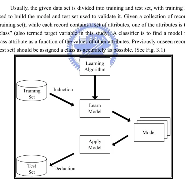
(23) CHAPTER3. METHODOLOGY. 3.1 Classification Model A classification technique (or classifier) is a systematic approach to building classification models from an input data set. Classification technique employs a learning algorithm to identify a model that best fits the relationship between the attribute set and class label of the input data. The model generated by a learning algorithm should both fit the input data well and correctly predict the class labels of records it has never seen before. Therefore, a key objective of the learning algorithm is to build models with good generalization capability; i.e., models that accurately predict the class labels of previously unknown records. (Tan et al., 2005) Usually, the given data set is divided into training and test set, with training set used to build the model and test set used to validate it. Given a collection of records (training set); while each record contains a set of attributes, one of the attributes is the “class” (also termed target variable in this study). A classifier is to find a model for class attribute as a function of the values of other attributes. Previously unseen records (test set) should be assigned a class as accurately as possible. (See Fig. 3.1) Learning Algorithm. Training Set. Induction Learn Model. Model Apply Model Test Set. Deduction. Figure 3.1 General Approach for Building a Classification Model Source: Tan et al., 2005.
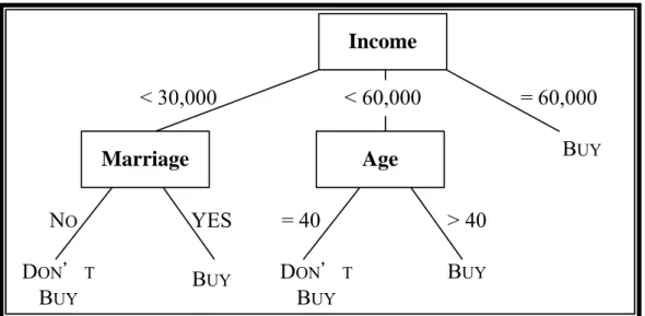
(24) Amongst other classification methods, decision trees have several advantages: 1. Simple to understand and interpret. Users are able to understand decision tree models after a brief explanation. 2. Able to handle both numerical and categorical data. Other techniques are usually specialized in analyzing datasets that have only one type of variable. (e.g.: Relation rules can be only used with nominal variables while neural networks can be used only with numerical variables.) 3. Achievable to use in high dimension data set. 4. Possible to validate a model using statistical tests. That makes it possible to account for the reliability of the model. 5. Decision trees are able to handle blank values. 6. Robust, perform well with large data in a short time. Large amounts of data can be analyzed using personal computers in a time short enough to enable users to take decisions based on its analysis.. 3.2 Decision Tree Induction Decision tree induction techniques are the most widely used classification/prediction methods and relatively small trees are easy to understand. Decision tree induction techniques build decision trees to label or categorize cases into a set of known classes. Decision tree induction techniques are well suited for high-dimensional applications and have strong explanation capabilities (Kim et al., 2002). In an induced decision tree, each non-leaf node denotes a test on an attribute, each branch corresponds to an outcome of the test, and each leaf node denotes a class prediction (see Figure 3.2). 17.
(25) Income < 30,000. < 60,000. Marriage. = 60,000 BUY. Age. NO. YES. = 40. > 40. DON'T BUY. BUY. DON'T BUY. BUY. Figure 3.2 An Example of Decision Tree There are well-known decision tree induction algorithms such as CHAID (Kass, 1980), CART (Breiman, 1984), C4.5 (Quinlan, 1993), etc. In this study, we choose to use C4.5 as decision tree induction algorithm. C4.5 is an algorithm improved from ID3 which was brought up by J. R. Quinlan in 1979. Not only is it a relatively new algorithm but a trendy post-pruning technique among other algorithms. There is a concept explanation of C4.5 in this section. C4.5 use “Entropy” based on ID3 to evaluate the degree of impurity, c −1. Entropy (t ) = −∑ p(i | t ) log 2 p(i | t ). (3.1). i =0. while p (i | t ) is the relative frequency of class i at node t. To determine how well a test condition performs, we need to compare the degree of impurity of the parent node (before splitting) with the degree of impurity of the child nodes (after splitting). The information gain, Δ , is a criterion that can be used to determine the goodness of a split: k. Δ Info = E ( parent ) − ∑. N (v j ). E (v j ) N E (⋅) is the Entropy of a given node.. (3.2). j =1. N is the total number of records at the parent node. k is the number of attribute values. N(v j ) is the number of records associated with the child node, v j. Since E(parent) is the same for all test conditions, maximizing the gain is equivalent to minimizing the weighted average impurity measures of the child nodes. 18.
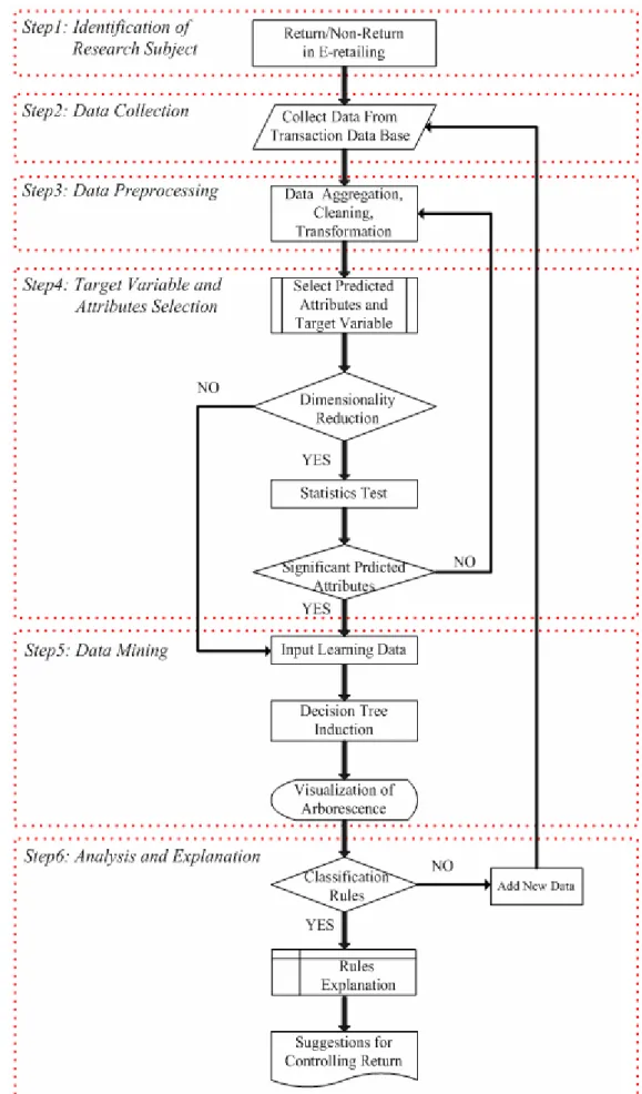
(26) When Entropy is used as the impurity measure in Equation 3.2, the difference in entropy is known as the Information Gain, Δ Info . The concept of Information Gain is used both in ID3 and C4.5. To maximize Information Gain, the algorithm tends to prefer splits that results in large number of partitions, each being small but pure. However, the large number of partitions may lead the number of record in each leaf node too small and the result unreliable. To overcome this problem, a splitting criterion known as Gain Ratio is used in C4.5 to adjust Information Gain by the Entropy of the partitioning. Namely, higher Entropy partitioning (large number of small partitions) is penalized. Δ Info Gain Ratio = (3.3) Split Info m. Split Info = −∑ P(vi ) log 2 P(vi ) i =1. m is the total number of split. Gain Ratio suggests that if an attribute produces a large number of splits, its split information will also be large, which in turn reduced its gain ratio.. 3.3 Research Framework Our analysis procedure of Decision Tree is presented in Figure3.3. There are six steps to complete the whole analysis procedure. First, we will start from case introduction to understand the return issue in real business and identify the target of this research. Further, data collection and data preprocessing are applied to assure the data quality. To continue, we will check the collinearity and correlation between each predicted variable and target variable. Then, we input the selected variables and target variable and build decision tree model. Finally, By way of arborescence visualization, we will conclude the findings of return rules and provide suggestion for strategy developing.. 19.
(27) Figure 3.3 Analysis Procedure of Decision Tree 20.
(28) CHAPTER4. EMPIRICAL DATA. 4.1 Case Introduction The online shopping website plays a role as an intermediary (defined in 2.1.1), which facilitates transactions between buyers and sellers and receives a fee for each transaction. It integrates the information of diversified retailers and the payment flow thus gains 2% margin from every successful transaction. The retailers consistently own the specific brand for their virtual stores and independently decide the inventory delivery approach and marketing strategies. There are more than 4,400 retailers in the website platform to sell more than 964,000 items (May, 2008) in this special case of E-retailing intermediary. In addition, there are approximately 150 new retailers joining the online shopping website per month. Since the profit of the online shopping website is mainly the fee charging from each successful transaction, the lower the return rate will bring higher marginal gains for the website company. Hence the online shopping website and the retailers cooperate to gain as much profits as possible. From the vision of the website manager, combing the whole information of customers, retailers and merchandise, this study plan to find out what’s the main factors differ the decisions of return. The results will be share with website managers and retailers.. 4.1.1. Order Procedure. The overall procedure of order in the online shopping website is explained as below and illustrated in Figure4.1: Payment flow and information flow between customers and retailers are facilitated by the website. Inventory flow is expedited by post or logistics providers. Step1: Each retailer updates merchandise information on web pages. Step2: Consumers browse the online shopping website and make an order. Step3: Consumers choose to pay the bill with three alternative provided by the website- ATM Transfer/Credit Card/Installment. Step4: Confirming the payment completed, the website management will 21.
(29) inform retailers to perform the inventory flow. Step5: Merchandise prepared and packaged by retailers. Step6: Retailers will deliver the items by Post or logistics service providers. Step7: There are two ways to deliver the merchandise to customers: one is traditional Home Delivery, and the other is oncoming Retail Delivery. Step8: Since the transaction is completed and a trial period is expired, the online shopping website will charge 2% of total transaction amount as its revenue. Retailers will receive the rest of 98% amount afterward.. Figure 4.1 Order Procedure of Online Shopping. 4.1.2. Return Procedure. The overall procedure of return in the online shopping website is explained as below and illustrated in Figure3.2: Payment flow and information flow between customers and retailers are still facilitated by the website. However, there is not a refund payment flow from retailers to the intermediary. This phenomenon is resulted from that intermediary would always pay the 98% of transaction amount to retailers after one week until confirming the 22.
(30) success of transaction. Inventory flow is expedited by post or logistics providers as well as order procedure. Step1: Customers claim to return merchandise online. Step2: Website management will inform retailers to contact with customers. Step3: Retailers connect with customers to send the returned merchandise by Post or take it by outsourced logistics service provider. Step4: Returned merchandise should be sent by Post or gathered by logistics service provider. Step5: Returned merchandise will be got back by retailers. Step6: Retailers will check the completeness of returned merchandise, recognize the reason of return and decide whether the merchandise is available for selling again. Step7: Retailers confirm the acceptance of return and inform website management to refund the money. Step8: Website management refunds the money to customers.. Figure 4.2 Return Procedure of Online Shopping. 23.
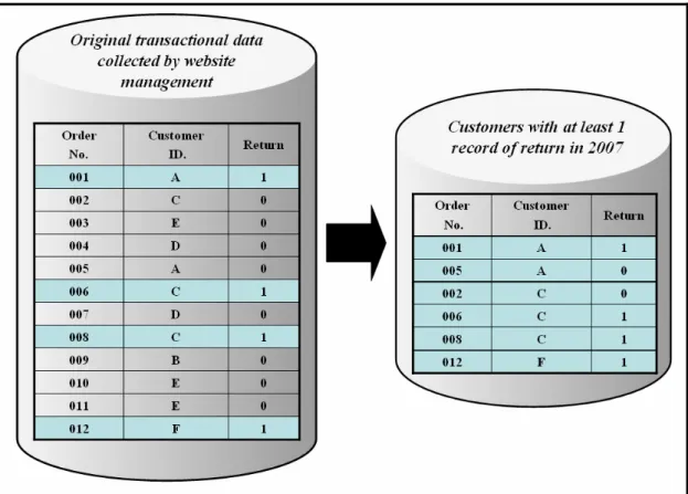
(31) 4.2. Data Collection. The data was collected during Jan., 2007 to Jan., 2008 by website management. The individual data in the selection were chosen on a basis that customers who had at least one return record between 2007. The observation data are collected by the customer ID as an index to involve his/her overall transaction records in 2007. The overall data record is 56,904 comprising 51,945 orders and 4,955 returns.. Figure 4.3 Data Collection Procedure. The original data is composed of four dimensions, covering customer demographic profile, merchandise characteristics, website/retailer services and transaction records. The customer demographic data includes gender, age, location, purchasing experience in online trading. The merchandise characteristics include price and category. The website/retailer services include payment, carriage, delivery approach, and evaluation function establish by the online shopping website. Finally, the target variable is measured by whether would be a return claim happened from transaction records. The original data is described as Table4.1.. 24.
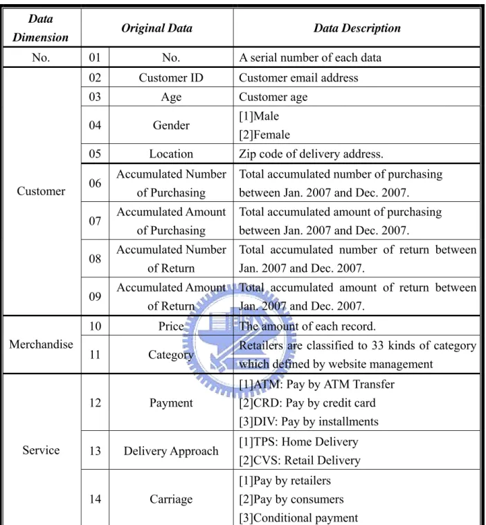
(32) Table 4.1 Description of Original Data Data Dimension. No.. Customer. Merchandise. Service. Original Data. Data Description. 01. No.. 02. Customer ID. 03. Age. 04. Gender. 05. Location. 06. Accumulated Number of Purchasing. Total accumulated number of purchasing between Jan. 2007 and Dec. 2007.. 07. Accumulated Amount of Purchasing. Total accumulated amount of purchasing between Jan. 2007 and Dec. 2007.. 08. Accumulated Number of Return. Total accumulated number of return between Jan. 2007 and Dec. 2007.. 09. Accumulated Amount of Return. Total accumulated amount of return between Jan. 2007 and Dec. 2007.. 10. Price. 11. Category. Retailers are classified to 33 kinds of category which defined by website management. 12. Payment. [1]ATM: Pay by ATM Transfer [2]CRD: Pay by credit card [3]DIV: Pay by installments. 13. Delivery Approach. [1]TPS: Home Delivery [2]CVS: Retail Delivery. Carriage. [1]Pay by retailers [2]Pay by consumers [3]Conditional payment. 14. A serial number of each data Customer email address Customer age [1]Male [2]Female Zip code of delivery address.. The amount of each record.. 25.
(33) Table 4.1(Con.) Description of Original Data Data Dimension. Original Data. Average Delivery Days. Evaluation function- Average delivery days of each retailer. Calculate the time of merchandise from retailers to delivery providers. Delivery days between delivery providers and customers are assumed to be constant.. 16. Accumulated Evaluation Score. Evaluation function- Customers could evaluate the retailer for each order. There are three levels to evaluate the satisfaction of customer: Good, Normal, and Bad, which are transformed to 1, 0, and -1. Thus it could be calculated to a sum of total score.. 17. Accumulated Number of Buyers. Evaluation function- total number of buyers of each retailer.. 18. Accumulated Number of Browsers. Evaluation function- total number of browsers of each retailer.. 19. Total Number of Merchandise. 20. Order Date. 21. Delivery Date. 22. Return Claim Date. 15. Service. Transaction. 4.3. Data Description. Evaluation function- total number of merchandise sold by each retailer. The date of order (yyyy/mm/dd) The date of delivery (yyyy/mm/dd) The date of claiming for return (yyyy/mm/dd). Data Preprocessing. There are some data preprocessing skills such as data generalization, discretizaion, aggregation and transformation etc. Transformation skill is used here to create new feature for better interpretable under our objective. For categorical data, data generalization is used to combine detailed data to more generalized form. In addition, statistics test and descriptive statistics analysis are used to review the continuous data to ensure a reasonable data quality. In this step, we eliminate the outliers and noise in original data, and exclude the collinear variables as well. The data preprocessing conclude the predicted variables into 3 dimensions and a target variable. 26.
(34) 1.. Customer Dimension. Zip code is generalized to county to present the variable - Location. There are two categorical variables- “Gender” and “Location”. Since we do not have domain knowledge about which age of people have higher return propensity, we keep continuous characteristic of age data. Consequently, there is one numeric variable- “Age” changed by eliminating outliers. 2.. Merchandise Dimension. One categorical variable- “Category” changed by eliminating noise and one numeric variable- “Price” are provided to describe merchandise dimension. 3.. Service Dimension. Statistics test shows that “Accumulated Evaluation Score” and “Accumulated Number of Buyer” are collinear (Tolerance = 0.09, VIF = 10.9). Hence, we choose Accumulated Number of Buyer to present the established customer base of each retailer’s. Moreover, we calculate a new variable- “Actual Delivery Days” by Delivery Date minus Order Date, and then discretize it from continuous data to ordinal data. In the same time, we switch the similar variables-“Average Delivery Days” to the same scale of data type. There are five categorical variables- “Payment”, “Delivery Approach”, “Carriage”, “Actual Delivery Days” and “Average Delivery Days.” Further, there are three numeric variables- “Accumulated Number of Buyers”, “Accumulated Number of Browsers”, and “Total Number of Merchandise.”. 4.3 Variable Explanation After data preprocessing, we finally decide the 13 predicted variables and one target variable as shown in Table 4.2.. 27.
(35) Table 4.2 Description of Input Variables Data Dimension. Customer. Merchandise. Variables. Data Type. 01. Age. Continuous. 02. Gender. Binary. [0] Female [1] Male. 03. Location. Nominal. 24 counties. 04. Price. Continuous. 05. Category. Nominal. 32 kinds of merchandise. 10 to 78. NT $1 to NT $180,000. 06. Payment. Nominal. [0] ATM: Pay by ATM Transfer [1] CRD: Pay by credit card [2] DIV: Pay by installments. 07. Delivery Approach. Nominal. [0] TPS: Home Delivery [1] CVS: Retail Delivery. Nominal. [0] Pay by retailers [1] Pay by Consumers [2] Conditional Payment. Ordinal. [0] Deliver on the order day [1] Deliver in 1 day [2] Deliver in 2 days [3] Deliver in 3 days [4] Deliver in 4 days [5] Deliver more than 5 days [0] Deliver on the order day [1] Deliver in 1 day [2] Deliver in 2 days [3] Deliver in 3 days [4] Deliver in 4 days [5] Deliver more than 5 days. 08. 09. Carriage. Actual Delivery Days. Service. Target. Data Description. 10. Average Delivery Days. Ordinal. 11. Accumulated Number of Buyers. Continuous. 1 to 13,611. 12. Accumulated Number of Browsers. Continuous. 0 to 12,656,670. 13. Total Number of Merchandise. Continuous. 0 to 15,344. 14. Return. Binary 28. [0] Non-return [1] Return.
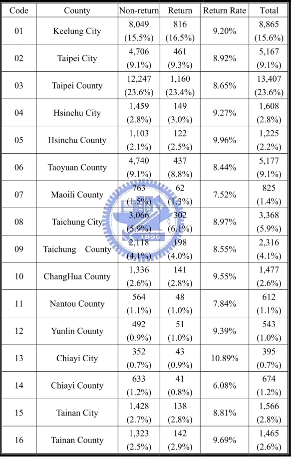
(36) 4.4. Data Analysis. The overall number of data in this analysis data set is 56,904 including 51,949 non-return orders and 4,955 returns. We define the target variable as 0 (non-return) and 1(return). The average return rate in this data set is 8.71% (4,955/56,904). Table 4.3 Target Variable Target. Non-return. Return. Return Rate. Total. Total. 51949 (100.0%). 4955 (100.0%). 8.71%. 56904 (100.0%). 4.5.1 Categorical Data Analysis of Cross Tabulation is conducted here to reveal general information of categorical data. 1. Gender. Female and male accounted for 30,535 (53.7%) and 26,369 (46.3%) of orders respectively. Orders from female customers are in the majority with slightly higher return rate in this data set. Table 4.4 Gender / Return Cross Tabulation Gender. Non-return. Return. Return Rate. Total. Female. 27,865 (53.6%). 2,670 (53.9%). 8.74%. 30,535 (53.7%). Male. 24,084 (46.4%). 2,285 (46.1%). 8.67%. 26,369 (46.3%). Total. 51,949 (100.0%). 4,955 (100.0%). 8.71%. 56,904 (100.0%). 2. Location. Taipei County (23.6%), Keelung City (15.6%), Tauyuan County (9.1%) and Taipei City (9.1%) are the main origins of orders (approximately 57%) in the whole data. In addition, there is a higher return propensity of customers from Chiayi City (10.89%), Hsinchu County (9.96%), Tainan County (9.69%). By contrast, return propensity of customers in Off-shore Islands (Penghu County, Kinmen 29.
(37) County) is relatively lower. Table 4.5 Location / Return Cross Tabulation Code. County. Non-return Return. Return Rate. Total. 01. Keelung City. 8,049 (15.5%). 816 (16.5%). 9.20%. 8,865 (15.6%). 02. Taipei City. 4,706 (9.1%). 461 (9.3%). 8.92%. 5,167 (9.1%). 03. Taipei County. 12,247 (23.6%). 1,160 (23.4%). 8.65%. 13,407 (23.6%). 04. Hsinchu City. 1,459 (2.8%). 149 (3.0%). 9.27%. 1,608 (2.8%). 05. Hsinchu County. 1,103 (2.1%). 122 (2.5%). 9.96%. 1,225 (2.2%). 06. Taoyuan County. 4,740 (9.1%). 437 (8.8%). 8.44%. 5,177 (9.1%). 07. Maoili County. 763 (1.5%). 62 (1.3%). 7.52%. 825 (1.4%). 08. Taichung City. 3,066 (5.9%). 302 (6.1%). 8.97%. 3,368 (5.9%). 09. Taichung County. 2,118 (4.1%). 198 (4.0%). 8.55%. 2,316 (4.1%). 10. ChangHua County. 1,336 (2.6%). 141 (2.8%). 9.55%. 1,477 (2.6%). 11. Nantou County. 564 (1.1%). 48 (1.0%). 7.84%. 612 (1.1%). 12. Yunlin County. 492 (0.9%). 51 (1.0%). 9.39%. 543 (1.0%). 13. Chiayi City. 352 (0.7%). 43 (0.9%). 10.89%. 395 (0.7%). 14. Chiayi County. 633 (1.2%). 41 (0.8%). 6.08%. 674 (1.2%). 15. Tainan City. 1,428 (2.7%). 138 (2.8%). 8.81%. 1,566 (2.8%). 16. Tainan County. 1,323 (2.5%). 142 (2.9%). 9.69%. 1,465 (2.6%). 30.
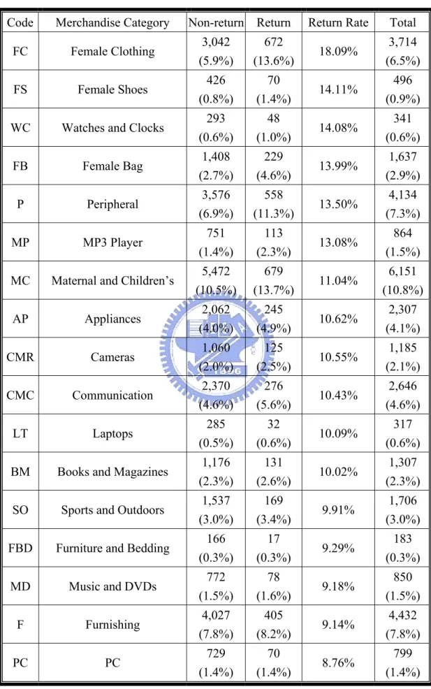
(38) Table 4.5(Con.) Location / Return Cross Tabulation Code. County. Return Rate. Total. 17. Kaohsiung City. 2,882 (5.5%). 271 (5.5%). 8.59%. 3,153 (5.5%). 18. Kaohsiung County. 1,279 (2.5%). 83 (1.7%). 6.09%. 1,362 (2.4%). 19. Pingtung County. 899 (1.7%). 64 (1.3%). 6.65%. 963 (1.7%). 20. Yilan County. 759 (1.5%). 80 (1.6%). 9.54%. 839 (1.5%). 21. Taitung County. 323 (0.6%). 31 (0.6%). 8.76%. 354 (0.6%). 22. Hualien County. 606 (1.2%). 56 (1.1%). 8.46%. 662 (1.2%). 23. Penghu County. 732 (1.4%). 53 (1.1%). 6.75%. 785 (1.4%). 24. Kinmen County. 90 (0.2%). 6 (0.1%). 6.25%. 96 (0.2%). 8.71%. 56,904 (100.0%). Total 3.. Non-return Return. 51,949 4,955 (100.0%) (100.0%). Merchandise Category. There are 32 kinds of merchandise in our data set. The most popular merchandises in the data set are: “Maternal and Child”, “Beauty” and “Food and Speciality” with the order ratios of 10.8%, 10.1%, and 8.1% respectively. “Female Clothing”, “Female Shoes”, “Watches and Clocks”, “Female Bags” and “Peripheral” have the highest return rate. It is obviously that merchandise related to female dressing needs a further observation.. 31.
(39) Table 4.6 Merchandise Category / Return Cross Tabulation Code. Merchandise Category. Non-return Return. Return Rate. Total. FC. Female Clothing. 3,042 (5.9%). 672 (13.6%). 18.09%. 3,714 (6.5%). FS. Female Shoes. 426 (0.8%). 70 (1.4%). 14.11%. 496 (0.9%). WC. Watches and Clocks. 293 (0.6%). 48 (1.0%). 14.08%. 341 (0.6%). FB. Female Bag. 1,408 (2.7%). 229 (4.6%). 13.99%. 1,637 (2.9%). P. Peripheral. 3,576 (6.9%). 558 (11.3%). 13.50%. 4,134 (7.3%). MP. MP3 Player. 751 (1.4%). 113 (2.3%). 13.08%. 864 (1.5%). MC. Maternal and Children’s. 5,472 (10.5%). 679 (13.7%). 11.04%. 6,151 (10.8%). AP. Appliances. 2,062 (4.0%). 245 (4.9%). 10.62%. 2,307 (4.1%). CMR. Cameras. 1,060 (2.0%). 125 (2.5%). 10.55%. 1,185 (2.1%). CMC. Communication. 2,370 (4.6%). 276 (5.6%). 10.43%. 2,646 (4.6%). LT. Laptops. 285 (0.5%). 32 (0.6%). 10.09%. 317 (0.6%). BM. Books and Magazines. 1,176 (2.3%). 131 (2.6%). 10.02%. 1,307 (2.3%). SO. Sports and Outdoors. 1,537 (3.0%). 169 (3.4%). 9.91%. 1,706 (3.0%). FBD. Furniture and Bedding. 166 (0.3%). 17 (0.3%). 9.29%. 183 (0.3%). MD. Music and DVDs. 772 (1.5%). 78 (1.6%). 9.18%. 850 (1.5%). F. Furnishing. 4,027 (7.8%). 405 (8.2%). 9.14%. 4,432 (7.8%). PC. PC. 729 (1.4%). 70 (1.4%). 8.76%. 799 (1.4%). 32.
(40) Table 4.6(Con.) Merchandise Category / Return Cross Tabulation Code. Merchandise Category. Return Rate. Total. VT. Video Games and Toys. 468 (0.9%). 38 (0.8%). 7.51%. 506 (0.9%). AT. Adult Toys. 1,442 (2.8%). 115 (2.3%). 7.39%. 1,557 (2.7%). CM. Cosmetic. 1,130 (2.2%). 81 (1.6%). 6.69%. 1,211 (2.1%). S. Stationery. 478 (0.9%). 33 (0.7%). 6.46%. 511 (0.9%). BG. Bouquet and Gift. 691 (1.3%). 46 (0.9%). 6.24%. 737 (1.3%). AM. Automotive. 945 (1.8%). 53 (1.1%). 5.31%. 998 (1.8%). PS. Pet Supplies. 1,203 (2.3%). 66 (1.3%). 5.20%. 1,269 (2.2%). CF. Collections and Fine Works. 429 (0.8%). 23 (0.5%). 5.09%. 452 (0.8%). OL. Ornament and Luxury. 3,010 (5.8%). 154 (3.1%). 4.87%. 3,164 (5.6%). FM. Flash Memory. 122 (0.2%). 6 (0.1%). 4.69%. 128 (0.2%). MF. Male Fashion. 234 (). 11 (0.2%). 4.49%. 245 (0.4%). B. Beauty. 5,546 (10.7%). 225 (4.5%). 3.90%. 5,771 (10.1%). CE. Computer Expendables. 920 (1.8%). 34 (0.7%). 3.56%. 954 (1.7%). HP. Health and Personal Care. 1,660 (3.2%). 49 (1.0%). 2.87%. 1,709 (3.0%). FS. Food and Speciality. 4,519 (8.7%). 104 (2.1%). 2.25%. 4,623 (8.1%). 8.71%. 56,904 (100.0%). Total. Non-return Return. 51,949 4,955 (100.0%) (100.0%). 33.
(41) 4.. Payment. Most of the transactions are paid by credit card (87.0%) with lowest return rate. There is a relatively higher return rate (12.27%) with transactions paid by installments while comparing to the others. Table 4.7 shows the difference of return rate for three kinds of payments. Table 4.7 Payment / Return Cross Tabulation. 5.. Payment Non-return Return. Return Rate. Total. DIV. 3,760 (7.2%). 526 (10.6%). 12.27%. 4,286 (7.5%). ATM. 2,793 (5.4%). 334 (6.7%). 10.68%. 3,127 (5.5%). CRD. 45,396 (87.4%). 4,095 (82.6%). 8.27%. 49,491 (87.0%). Total. 51,949 4,955 (100.0%) (100.0%). 8.71%. 56,904 (100.0%). Delivery Approach. Since the retail delivery is a new approach for customers to choose, there is an obviously unbalanced ratio between the two alternatives. However, a significant higher return rate belonged to retail delivery is worth for a further analysis. Table 4.8 Delivery Approach / Return Cross Tabulation Delivery Approach Non-return Return. Total. CVS-Retail Delivery. 209 (0.4%). 32 (0.6%). 13.28%. 241 (0.4%). TPS-Home Delivery. 51,740 (99.6%). 4,923 (99.4%). 8.69%. 56,663 (99.6%). 51,949 4,955 (100.0%) (100.0%). 8.71%. 56,904 (100.0%). Total 6.. Return Rate. Carriage. Approximately 67.8% of the data are paid by customers, and the remaining are relatively distributed across free-carriage (14.6%) and conditional payment (17.7%).. 34.
(42) There is the highest return rate while the carriage is paid by conditions (e.g., the retailer will afford the carriage if the amount of data is higher than NT $1,000). Table 4.9 Carriage / Return Cross Tabulation Carriage. Return Rate. Total. Conditional. 8,908 (17.1%). 1,159 (23.4%). 11.51%. 10,067 (17.7%). Pay by Customers. 35,376 (68.1%). 3,178 (64.1%). 8.24%. 38,554 (67.8%). Pay by Retailers. 7,665 (14.8%). 618 (12.5%). 7.46%. 8,283 (14.6%). 51,949 4,955 (100.0%) (100.0%). 8.71%. 56,904 (100.0%). Total 7.. Non-return Return. Actual Delivery Days. The frequency of Actual Delivery Days spreads from “0” day to “268” days. Moreover, the frequency more than “5 days” is much fewer than the first five levels (0, 1, 2, 3, and 4). Further, to separate the delivery fewer than and more than 5 workdays, we decide to discretize the variable to six levels-0, 1, 2, 3, 4, and more than 5. In the Table 4.10, there is an obvious phenomenon that the return rate becomes higher as the Actual Delivery days increases. Actual Delivery days equals 2 days deserve almost the same return rate as average, while Actual Delivery more than 5 days has 1.5 times higher return rate compared to average. Table 4.10 Actual Delivery Days / Return Cross Tabulation Actual Delivery Non-return Return Days. Return Rate. Total. 0. 15084 (29.0%). 1239 (25.0%). 7.59%. 16323 (28.7%). 1. 18139 (34.9%). 1554 (31.4%). 7.89%. 19693 (34.6%). 2. 7635 (14.7%). 729 (14.7%). 8.72%. 8364 (14.7%). 3. 4734 (9.1%). 502 (10.1%). 9.59%. 5236 (9.2%). 35.
(43) Table 4.10(Con.) Actual Delivery Days / Return Cross Tabulation Actual Delivery Non-return Return Days. Total. 4. 3583 (6.9%). 499 (10.1%). 12.22%. 4082 (7.2%). More than 5. 2774 (5.3%). 432 (8.7%). 13.47%. 3206 (5.6%). 8.71%. 56904 (100.0%). Total 8.. Return Rate. 51949 4955 (100.0%) (100.0%). Average Delivery Days. The frequency of Average Delivery Days spreads from “0” day to “14” days. In the same way, the frequency more than “5 days” is much fewer than the first five levels (0, 1, 2, 3, and 4). To compare with “Actual Delivery Days”, therefore, we discretize the variable to six levels-0, 1, 2, 3, 4, and more than 5 as last variable. Orders delivered in 1 or 2 days occupy the major percentage of Average Delivery Days (more than 70%), while only a few orders supplied by some specific retailers are delivered more than 5 days (1.86%). Table 4.11 Average Delivery Days / Return Cross Tabulation Ave. Delivery Non-return Return Days. Return Rate. Total. 0. 3,728 (7.18%). 389 (7.85%). 9.45%. 4,117 (7.23%). 1. 19,519 1,391 (37.57%) (28.07%). 6.65%. 20,910 (36.75%). 2. 18,912 1,779 (36.40%) (35.90%). 8.60%. 20,691 (36.36%). 3. 5,791 660 (11.15%) (13.32%). 10.23%. 6,451 (11.34%). 4. 3,055 (5.88%). 623 (12.57%). 16.94%. 3,678 (6.46%). More than 5. 944 (1.82%). 113 (2.28%). 10.69%. 1,057 (1.86%). Total. 51,949 (100%). 4,955 (100%). 8.71%. 56,904 (100%). 36.
(44) 4.5.2 Continuous Data Analysis of Descriptive Statistics is conducted here to reveal general information of continuous data. 1.. Age. The average age of customers is 35 years old. The upper bound of age is 78 and the lower bound is 10. Distribution of Age data shown in figure 4.4 reveals that people at 27 to 40 years old are the main customers who accounted for approximately 60% of orders. 4,000. Frequency. 3,000. 2,000. 1,000. 0 7 9 11 13 15 17 19 21 23 25 27 29 31 33 35 37 39 41 43 45 47 49 51 53 55 57 59 61 63 65 68 71 73 77 85 87. Age. Figure 4.4 Distribution of Age Data 2.. Price. The average price of each data is NT $1,724. The maximum is NT $180,000 and the minimum is NT $1. The lowest price among the items is NT $1, which is resulted from trail or promotion. Customers only need to pay for NT $1 plus the carriage. 3.. Accumulated Number of Buyers. This variable represents the established reputation of each retailer. The accumulated number of buyers of each retailer is 1,590. The maximum is 13,611 and the minimum is 1.. 37.
(45) 4.. Accumulated Number of Browsers. The average accumulated number of browsers of each retailer is 132,256. The maximum is 12,656,670 and the minimum is 11. 5.. Total Number of Merchandise. The average number of merchandise of each retailer is 713. The maximum is 15,344 and the minimum is 0.. 38.
(46) CHAPTER5. RESULTS AND ANALYSIS. 5.1 Setup and Sampling In this study, we use SAS Enterprise Miner vision 4.1 to conduct classification. As we mentioned in Section 3.2, C4.5 is selected to be the algorithm while conducting decision tree induction. C4.5 relies on Entropy reduction as a splitting criterion. “Maximum number of branches from a node” and “maximum depth of tree” are set at “3” and “4” to control Decision Trees not to be simplistic or too complicated. “Minimum number of observations in a leaf” and “Observations required for a split search” are also controlled to avoid over-fitting and trivial rules. Full information is given in Table 5.1. Table 5.1 Information of Decision Tree Setting Software. SAS Enterprise Miner. Splitting criterion. Entropy (C4.5). Maximum number of branches from a node. 3. Maximum depth of tree. 4. Proportion. Training. 50%. Validation. 20%. Test. 30%. The data analysis mentioned before indicated that this problem is a binary choice model with a skewed distribution. The number of “Return” is noticeably less than “Non-return”. Thus, we use the whole “Return” data and sample from the “Non-return” data to lead the ratio of each other equal 1:1. For example, there are 30,573 orders from female customers, while 2,668 were return and 27,905 were not return. To solve the unbalance problem, thus, we sample the same number of samples from non-return orders (2,668/27,905).. 39.
(47) Figure 5.1 Data Sampling. 5.2 Model Development In this section, we try five kinds of trees according to customer feature- Gender and Total Number of Transaction in 2007; and merchandise feature- category. The reason to choose these five groups to develop decision tree will be explained before each section. General information about DTs is comprehended in Table 5.2. Rules within “Return” label more than 50% mean that the transaction has higher possibility to be cancels by return the goods. In this situation, special attention is required to analyze it. Table 5.2 General Information of Decision Trees DT Types Variables. Total Number of Female Transaction in 2007 Merchandise. Gender Female. Male. ≤ 12. > 12. Minimum number of observations in a leaf. 50. 50. 60. 40. 20. Observations required for a split search:. 100. 100. 120. 80. 40. Number of Samples. 5336. 4582. 6098. 3828. 1942. Accuracy of Training. 65.63%. 63.25%. 62.16%. 69.80%. 67.25%. Accuracy of Validation. 63.07%. 60.04%. 56.20%. 65.80%. 67.53%. Accuracy of Test. 63.96%. 59.56%. 60.67%. 62.37%. 65.87%. Number of Leaf Node. 19. 11. 13. 17. 9. Return Leaf Node. 10. 6. 8. 10. 3. Non-Return Leaf Node. 9. 5. 5. 7. 6. 40.
(48) 1. Gender. Since “Gender” is an important feature for retailer to target their major customers, we separate Female and Male data to two groups to distinguish the difference between them. (1) Female. The average number of transaction of female customer in 2007 is 14.9 while the average number of return is 1.5. The average amount of transaction of female customers in 2007 is NT $22,699 while the average amount of return is NT $2,313. The rules which display more than 50% of return propensity for female customers are described as Table 5.3. Table 5.3 Selected Rules of Decision Tree-Female Customers THEN… No.. R1. R2. R3. R4. R5. Number. Rules (IF…). Class Label. Percentage of Training. IF 2 ≤ Ave. Delivery Days < 3 AND Category is one of: MP PC FC FS CMR MD VT. Sample. 109. Return. 67.0%. Non-Return. 33.0%. IF 3 ≤ Ave. Delivery Days AND Category is one of: MP PC FC FS CMR MD VT. Sample. 120. Return. 82.5%. Non-Return. 17.5%. IF 649.5 ≤ Price < 1,998 AND Category is one of: FB WC SO F CE MC P IF 1,998 ≤ Price AND Category is one of: FB WC SO F CE MC P IF 338 ≤ Price < 1,614.5 AND Ave. Delivery Days < 2 AND Category is one of: MP PC FC FS CMR MD VT. 41. Sample. 439. Return. 60.6%. Non-Return. 39.4%. Sample. 186. Return. 76.9%. Non-Return. 23.1%. Sample. 202. Return. 60.4%. Non-Return. 39.6%.
(49) Table 5.3(Con.) Selected Rules of Decision Tree-Female Customers THEN… No.. R6. R7. R8. R9. Number. Rules (IF…). Class Label. Percentage of Training. IF 1,614.5 ≤ Price AND Ave. Delivery Days < 2 AND Category is one of: MP PC FC FS CMR MD VT. Sample. 53. Return. 75.5%. Non-Return. 24.5%. IF Location is one of: 7 8 9 12 13 16 20 21 22 AND Price < 649.5 AND Category is one of: FB WC SO F CE MC P. Sample. 65. Return. 64.6%. Non-Return. 35.4%. IF AND AND AND. Num. of Merchandise < 257.5 Location is one of: 1 2 4 5 6 10 17 Price < 649.5 Category is one of: FB WC SO F CE MC P. IF AND AND AND. 701 ≤ Num. of Merchandise Location is one of: 1 2 4 5 6 10 17 Price < 649.5 Category is one of: FB WC SO F CE MC P. IF 1,098 ≤ Price < 1,559 AND Location is one of: 1 2 3 5 6 7 8 10 14 17 23 R10 AND Category is one of: S CF AM BG HP B CM FS AP BM AT CMC OL FM PS. Sample r. 66. Return. 51.5%. Non-Return. 48.5%. Sample. 53. Return. 60.4%. Non-Return. 39.6%. Sample. 82. Return. 54.9%. Non-Return. 45.1%. (2) Male. The average number of transaction of male customer in 2007 is 13.6 while the average number of return is 1.4. The average amount of transaction of male customers in 2007 is NT $20,519 while the average amount of return is NT $2,822.9. The rules which display more than 50% of return propensity for male customers are described as Table 5.4.. 42.
(50) Table 5.4 Selected Rules of Decision Tree- Male Customers THEN… No.. R1. R2. R3. R4. R5. R6. Number. Rules (IF…). Class Label. Percentage of Training. IF 230 ≤ Price < 1,776.5 AND Category is one of: LT FB SO AM F BG B CMR AP MC AT CMC OL PS. Sample. 712. Return. 52.8%. Non-Return. 47.2%. IF 1,776.5 ≤ Price AND Category is one of: LT FB SO AM F BG B CMR AP MC AT CMC OL PS. Sample. 315. Return. 64.8%. Non-Return. 35.2%. IF 1,615.5 ≤ Num. of Merchandise AND Category is one of: MP PC FC FS WC S CM BM VT P. Sample. 148. Return. 79.7%. Non-Return. 20.3%. IF 442 ≤ Accum. Buyer < 1,118 AND Num. of Merchandise < 551.5 AND Category is one of: MP PC FC FS WC S CM BM VT P. Sample. 166. Return. 72.3%. Non-Return. 27.7%. IF Accum. Buyer < 575 AND 551.5 ≤ Num. of Merchandise < 1,615.5 AND Category is one of: MP PC FC FS WC S CM BM VT P IF AND AND AND. Age < 38.5 1118 ≤ Accum. Buyer Num. of Merchandise < 551.5 Category is one of: MP PC FC FS WC S CM BM VT P. Sample. 50. Return. 66.0%. Non-Return. 34.0%. Sample. 58. Return. 62.1%. Non-Return. 37.9%. 2. Total Number of Transaction in 2007. Due to the restriction of our data set, we use total number of transaction in 2007 to distinguish the transaction frequency of each customer. Once per month is the threshold for determining whether he/she is a high frequency buyer or not. (1) Equal to or less than 12 times. We define the customer whose frequency of transaction in 2007 is equal to or less than 12 as our potential customers. To effectively reduce the return rate of this group customer, we need to understand what the critical factors 43.
(51) revealing their return propensity are. The average number of transaction of low-transaction frequency customer in 2007 is 6.2 while the average number of return is 1.2. The average amount of transaction of this group in 2007 is NT $10,625 while the average amount of return is NT $2,388. The rules which display more than 50% of return propensity for low-transaction frequency customers are described as Table 5.5. Table 5.5 Selected Rules of Decision Tree- Low Frequency Customers THEN… No.. R1. R2. R3. R4. R5. R6. R7. Number. Rules (IF…). Class Label. IF 2,890 ≤ Price AND Category is one of: MP FB WC SO F BG B CMR AP BM MC AT CMC P OL IF Ave. Delivery Days = 3 AND Category is one of: FC FS S AM MD FBD IF 4 ≤ Ave. Delivery Days AND Category is one of: FC FS S AM MD FBD IF Num. of Merchandise < 135.5 AND 242.5 ≤ Price < 2,890 AND Category is one of: MP FB WC SO F BG B CMR AP BM MC AT CMC P OL. Percentage of Training. Sample. 315. Return. 57.5%. Non-Return. 42.5%. Sample. 92. Return. 72.8%. Non-Return. 27.2%. Sample. 94. Return. 81.9%. Non-Return. 18.1%. Sample. 288. Return. 50.3%. Non-Return. 49.7%. IF 135.5 ≤ Num. of Merchandise < 1,039.5 AND 242.5 ≤ Price < 2,890 AND Category is one of: MP FB WC SO F BG B CMR AP BM MC AT CMC P OL. Sample. 840. Return. 60.5%. Non-Return. 39.5%. IF 988.5 ≤ Price AND Ave. Delivery Days < 2 AND Category is one of: FC FS S AM MD FBD. Sample. 106. Return. 65.1%. Non-Return. 34.9%. IF AND AND AND. Ave. Delivery Days = 2 1,039.5 ≤ Num. of Merchandise 242.5 ≤ Price < 2,890 Category is one of: MP FB WC SO F BG B CMR AP BM MC AT CMC P OL 44. Sample. 158. Return. 51.3%. Non-Return. 48.7%.
數據
+7

相關文件
In the second quarter of 2003, the average number of completed units in each building was 11, which was lower than the average value for 2002 (15 units). a The index of
Chang-Yu 2005 proves that the Euler-Carlitz relations and the Frobenius relations generate all the algebraic relations among special Carlitz zeta values over the field ¯ k.. Jing
To take the development of ITEd forward, it was recommended in the Second Information Technology in Education Strategy “Empowering Learning and Teaching with Information
(b) If, in a particular year, the accumulated surplus of the grant reaches 500% of the current year provision, EDB will suspend the disbursement of grant and claw back the
利用 determinant 我 們可以判斷一個 square matrix 是否為 invertible, 也可幫助我們找到一個 invertible matrix 的 inverse, 甚至將聯立方成組的解寫下.
Process: Design of the method and sequence of actions in service creation and delivery. Physical environment: The appearance of buildings,
Joint “ “AMiBA AMiBA + Subaru + Subaru ” ” data, probing the gas/DM distribution data, probing the gas/DM distribution out to ~80% of the cluster. out to ~80% of the cluster
By this, the second-order cone complementarity problem (SOCCP) in H can be converted into an unconstrained smooth minimization problem involving this class of merit functions,
