系統風險、公司規模、帳面市值比、風險值和股票報酬的關係:以台灣股票市場為例

國

立 交 通 大 學

財 務 金 融 研 究 所

碩 士 論 文

系統風險、公司規模、帳面市值比、風險值和股票報酬的關係

:

以台灣股票市場為例

A reexamination of Market Beta, Firm Size, Book-to-Market,

Value-at-Risk in Stock Returns:

Evidence from the Taiwan Stock Market

研 究 生：吳素禎

指導教授：陳達新 博士

中

華 民 國 九 十 五 年 六 月

系統風險、公司規模、帳面市值比、風險值和股票報酬的關係

:

以台灣股票市場為例

A reexamination of Market Beta, Firm Size, Book-to-Market,

Value-at-Risk in Stock Returns:

Evidence from the Taiwan Stock Market

研 究 生: 吳素禎 Student: Su-Chen Wu

指導教授: 陳達新博士 Advisor: Dr. Dar-Hsin Chen

國立交通大學

財務金融研究所碩士班

碩士論文

A Thesis

Submitted to Graduate Institute of Finance

National Chiao Tung University

in partial Fulfillment of the Requirements

for the Degree of

Master of Science

in

Finance

June 2006

Hsinchu, Taiwan, Republic of China

系統風險、公司規模、帳面市值比、風險值和股票報酬的關係

:

以台灣股票市場為例

學生:吳素禎 指導教授:陳達新 博士 國立交通大學財務金融研究所碩士班 2006 年 6 月 摘要 本研究利用橫斷面時間序列分析法探討台灣股票市場上:市場因素、規模效 應、股價淨值比效應和風險值因素對股票市場報酬的解釋力，主要目的是要加入 新的風險指標—風險值，形成四因子模型，利用時間序列分析此因子對台灣股市 報酬的解釋力及影響方向，對模型的總解釋力影響為何。實證結果發現，利用歷 史模擬法所算出的風險值，在橫斷面分析時，1%和 5%顯著水準之下，具有解釋 能力，而在時間序列分析方面，若分成25 投資組合來看，對大規模公司而言， 風險值因子對投資組合期望報酬率較具有解釋力。 關鍵字: 資本資產定價模式; 系統風險;異常現象;台灣股票市場; 風險值

A reexamination of Market Beta, Firm Size, Book-to-Market,

Value-at-Risk in Stock Returns:

Evidence from the Taiwan Stock Market

Student: Su-Chen Wu Advisor: Dr. Dar-Hsin Chen

Graduate Institute of Finance June 2006

ABSTRACT

This paper investigates the explanatory power of the market beta, firm size, and the book-to-market ratio, as well as Value-at-Risk regarding the cross-sectional expected stock returns in the Taiwan stock market. Our primary objective is to determine whether the Value-at-Risk factor has marginal explanatory power that is related to the Fama-French three-factor model. This study finds that Value-at-Risk can explain average stock returns at the 1% and 5% significance levels based on cross-sectional regression analysis. In addition, from the perspective of the time series regression, the HVARL factor can also help explain the variation in the stock market, especially for the larger companies in Taiwan’s stock market.

誌

謝

天下沒有不散的宴席，又到鳳凰花開、驪歌響起的季節，在研究所兩年的生 涯，有甘有苦，但在大家的陪伴之下，苦中都會帶有友情的支柱，一同克服化解 苦澀、困難，使得最終能有很圓滿的結果，隨著即將劃上一個完美的句點，即將 面對人生一個新的啟程，這份成果是大家給予的，謹將這份成果獻給曾經幫助我 的人，謝謝你們讓我完成人生之一大理想。 這份論文能順利完成，首先要感謝指導教授陳達新博士，給我論文的方向， 並且指正我從論文觀念啟發到論文架構建立至最後成果完成，給我細心的指導， 並且感謝口試委員林建榮老師、周德瑋老師和劉祥熹老師給予建議和勉勵，使本 論文能更趨完善，在此特別向以上四位老師致上最真誠的謝意。 研究期間，承蒙好友尚育和柏鈞給予程式上的幫助，忠穎班長給予論文觀念 的解析及協助，以及摯友于倢、慧妤、怡文陪伴我渡過難熬的時光，在我沮喪或 心情低落時，給我鼓勵及支持，以及交大財金所一群熱情的朋友，這多采多姿的 研究生活，若少了你們，我的生活將無法過得如此幸福，因為你們讓我更加勇敢 的面對我的夢想，完成本篇論文，在此獻上我最深的謝意，並誠摯祝福大家。 最後，最最最感謝的是我的家人，因為有你們的支持，才有今日的我，所以 這份成就是你們給我的，在此，將最後的小小的成果，獻給我的家人，以回報培 育之恩。 素禎 于交通大學 2006 年 6 月

Contents

中文摘要

...i

英文摘要

... ii

誌

謝 ... iii

Contents ... iv

List of Tables ... vi

List of Figures... vii

1. Introduction...1

2. Literature Review ...4

2.1 Systematic Risk (Beta)...5

2.2 Size Effect ...6

2.3 Book-to-Market Equity (BE/ME)...7

2.4 Value-at-Risk (VaR) ...9

3. Data and Variable Definitions ...10

3.1 Data ...10

3.2 Variable Definitions ...10

4. Methodology and Models ...14

4.1 Cross-Sectional Regression ...14

4.2 Inputs to the Time Series Regression ...15

4.3 Main Model...17

5. Empirical Results...20

5.1 VaR and Cross–Sectional Regression ...20

5.2 VaR and Time-Series Variation of Expected Returns...21

5.3 Properties of Portfolios Formed Based on Size and Pre-ranking β ...22

5.5 Main Model Results: Factor Models ...24

6. Conclusions and Comments...27

References...29

List of Tables

Table 1: Cross-Sectional Regressions of Stock Returns on Beta, Size, BE/ME, and VaR ...33 Table 2: Time Series Regressions -- Simple Statistics...34 Table 3: Correlations of 25 Portfolio Returns with RMRF, SMB, HML and

HVARL ...35 Table 4: Properties of Portfolios Formed on Size and Pre-ranking β: Stocks

Sorted by Size (Down) then Pre-ranking β (Across), 1996-2004 ...36 Table 5: Properties of Portfolios Formed on VaR and Pre-ranking β: Stocks

Sorted by VaR (Down) then Pre-ranking β (Across), 1996-2004 ...37 Table 6: One-Factor Model: Regression of Excess Stock Returns on the Excess

Stock-Market Return, HVARL, SMB and HML (January 1996 to

December 2004, n=108) ...38 Table 7: Two-Factor Model: Regression of Excess Stock Returns on the Excess

Stock-Market Return and HVARL/ SMB / HML (January 1996 to December 2004, n=108) ...41 Table 8: Three-Factor Model: Regression of Excess Stock Returns on the Excess

Stock-Market Return, SMB, and HML (January 1996 to December 2004, n=108)...44 Table 9: Four-Factor Model: Regression of Excess Stock Returns on the Excess

Stock-Market Return, SMB, HML, and HVARL (January 1996 to December 2004, n=108) ...45

List of Figures

Figure 1: The Industry Distributions of the Total Sample (N=133)...47 Figure 2: Average Return of the Portfolios Sorted on 1% VaR (January 1996 to

December 2004)...48 Figure 3: Average Return of the Portfolios Sorted on 5% VaR (January 1996 to

December 2004)...49 Figure 4: Average Return of the Portfolios Sorted on 10% VaR (January 1996 to December 2004)...50

1. Introduction

The validity of modern portfolio theory has been and will continue to be an important research issue. The tradeoff between risk and expected return, which can be viewed as a “No free lunch” principle, asserts that over the long run it is not possible to achieve exceptional returns without accepting commensurably substantial risks. Any standard equilibrium model of asset pricing justifies this relationship. The well- known capital asset pricing model (CAPM) of Sharpe (1964), Linter (1965), and Black (1972) has, for decades, been the major framework for analyzing the cross sectional variation in expected asset returns. The main implication of the theory is that: (a) the expected return on a security is a positive linear function of its market β and (b) the market β itself suffices to describe the cross-section of expected returns.

Unfortunately, theory and practice do not always match. Fama and French (1992) drew two negative conclusions regarding CAPM, namely: (a) when one allows for variations in CAPM market βs that are unrelated to size, the univariate relationship between β and the average return for 1941-1990 is weak, and (b) β does not suffice to explain the average return. Fama and French further find no cross-sectional mean-beta relationship after controlling for size and the ratio of book-to-market equity. The evidence shows that the market return should not be the only relevant risk factor in the economy, and additional factors are required to explain the expected returns.

Several alternative risk factors have consequently been employed in the literature, for example, the size effect of Banz (1981). He finds that the market value of equity (ME) provides a prominent explanation of the cross-section of average returns provided by market beta. Variables such as the book-to-market equity ratio (BE/ME) (Fama and French, 1992, 1993, 1995, 1996; Stattman, 1980; Rosenberg, Reid, and Lanstein, 1985), the price/earnings ratio (Basu, 1977), leverage (Bhandari, 1998), and

Value-at-Risk (Bali and Cakici, 2004) all have significant explanatory power for explaining average expected returns.

In particular, the concept and use of Value-at-Risk (henceforth VaR) is relatively recent and is designed to summarize the predicted maximum loss (or worst loss) over a target horizon within a given confidence interval (Jorion, 2000). Extreme price movements are rare, but they can bring serious results to some corporations, leading to disastrous consequences for a country’s financial markets. For instance, the New York stock market crashed in October 1987, and then, one decade later, the Asian stock market crashed in 1997. Besides, the Enron scandal has also caused the Dow Jones Industrial Average (DJIA) to drop sharply. These crises have harmed thousands of companies and much of the value of their stocks has been wiped out within a short period of time. Therefore, to a risk manager, a good measure of market risk is more than necessary. VaR was first used by major financial firms in the late 1980’s to measure the risks of their trading portfolios. Since then, the use of VaR has exploded, with J.P. Morgan’s attempt to establish a market standard through its release of the RiskMetricsTM system in 1994.

VaR is now not only widely used by financial institutions, non-financial corporations, and institutional investors, but has also become a common language for communication with regard to aggregate risk taking, both within an organization and outside it (for example, with analysts, regulators, and shareholders). Even regulators have become interested in VaR. For example, the Basle Committee on Banking Supervision (Basle Committee, 1996) permits banks to calculate their capital requirements for market risk using their own proprietary VaR models, while the Securities and Exchange Commission (SEC, 1997) requires that U.S. companies disclose quantitative measures of market risks, with VaR listed as one of three possible market risk disclosure measures.

In a normal world, the standard deviation of the portfolio returns is a good risk measure, and efficient portfolios are the ones generating the best mean-variance profiles. Modeling portfolio risk with traditional standard deviation measures implies that investors are concerned only with the average variation in individual stock returns, and they are not allowed to treat the negative and positive tails of the return distribution separately. However, statistical data exhibit fat-tailed and asymmetric distributions for market returns. The fat tail represents the extent to which the portfolio’s value can be affected by large jumps in market prices. The empirical evidence also indicates that the minimum-variance portfolios are far from being the most efficient ones with respect to the relevant risk measures. During the last few decades we can see that the most popular and traditional measure of risk has been volatility. The main problem with volatility, however, is that it does not take into consideration the direction of an investment’s movement － a stock can be volatile because it suddenly jumps higher. However, investors are not distressed by gains! By assuming that investors care about the likelihood of a really big loss, VaR answers the question, “What is my worst-case scenario?”

Traditional models treat all uncertainty as risk, regardless of the direction it takes. As many people have shown, that is a problem if returns are not symmetrical – investors worry about their losses “to the left” of the average, but they do not worry about their gains “to the right” of the average. If investors are more averse to the risk of losses on the downside than to the gains on the upside, investors ought to demand greater compensation for holding stocks with greater downside risk. In particular, many authors, including Campbell, et al. (2001), find that market volatility increases in bear markets and recessions. Moreover, Duffee (1995) finds that idiosyncratic volatility decreases in down-markets. Both of these effects cause the conditional beta to have little asymmetry across the downside and the upside. To

sum up, this paper measures VaR in terms of a company’s market value at risk. Hence the VaR is related to the company’s stock price and it thus reflects the shareholders’ perception of risk. The reason for considering VaR is that it is an easy-to-understand summary measure of downside risk. The downside focus separates the loss from the upside potential － only the former truly constitutes risk and only negative surprises to the stock market represent potential litigation threats. Furthermore, the concept of VaR is easily grasped and hence easily communicated.

Surprisingly, despite its wide acceptance among practitioners, academics, and regulators, VaR has so far only been considered to be a risk factor in Bali and Cakici’s (2004) study. Therefore, this research aims to supplement our understanding of the measurement of risk and to provide some emerging market evidence while the only related study focuses mainly on mature markets. The Taiwan stock market is also unique for its tight short-sale constraints and a 7% daily price change limit.

An important contribution of this paper is that it tests whether the maximum likely loss measured by VaR plays a key role in explaining expected returns in Taiwan. The central motivation behind this paper is that it also provides an analysis in terms of examining the cross-sectional variation among beta, firm size, the book-to-market ratio (BE/ME) and Value-at-Risk (VaR) at the firm level. The remainder of this paper is organized as follows. Section 2 reviews the literature. Section 3 describes the dataset and variable definitions. Section 4 contains the methodology and models. Section 5 presents the empirical results of our analysis. Section 6 summarizes and concludes our findings.

2. Literature Review

Empirical research has provided several pieces of evidence that reject the validity of the Sharpe-Linter capital asset pricing model (CAPM). The existence of market

frictions, the presence of irrational investors and inefficient markets may distort the cross-sectional relationship between expected stock returns and market return. This research will discuss the related evidence that has been reported in empirical studies.

2.1 Systematic Risk (Beta)

Beta, or the sensitivity of asset returns to underlying sources of risk, is central to modern finance. Beta has been used by academics and practitioners to model and measure systematic risk. Sharpe (1964) and Linter (1965) found a positive and a linear function between the expected returns on securities and their betas. Miller and Scholes (1972), Black, Jensen, and Scholes (1972), and Fama and MacBeth (1973) all empirically confirmed a positive relationship between mean returns and betas across firms.

Subsequently, Reinganum (1981) found that estimated betas were not systematically related to average returns across New York Stock Exchange and American Stock Exchange securities. In the 1990s, however, much controversy was stirred in the finance literature as if beta completely lacked predictive power for expected returns. For instance, Fama and French (1992) also found evidence that the relationship between the average return and beta for common stocks was even flatter after the sample periods used in the early empirical work on the CAPM, and that the relationship between beta and the average return was flat, even when beta was the only explanatory variable. Kothari, Shanken, and Sloan (1995) tried to resuscitate

the Sharpe-Lintner CAPM by arguing that the weak relationship between the average return and beta came about just by chance. However, the strong evidence that other variables captured the variation in expected return missed by beta made this argument irrelevant. By investigating international findings, Heston, Rouwenhorst, and Wessels (1999) examined the ability of beta and size to explain cross-sectional variation in average returns in 12 European countries. They found that average stock

returns were positively related to beta and negatively related to firm size. The beta premium was in part due to the fact that high beta countries outperformed low beta countries. Within countries, high beta stocks outperformed low beta stocks only in

January, but not in other months. The differences in the average returns of the size- and beta-sorted portfolios could not be explained by market risk and exposure to the excess return of small over large stocks (SMB)1.

2.2 Size Effect

The size effect is the most well-known empirical inconsistency of the CAPM. The size premium for small-cap firms is one of the market anomalies and was originally discovered by Banz (1981). The evidence showed that the stock returns of firms with small-cap market capital (size) had statistically higher returns than firms with large-cap market capital and the CAPM beta could not justify this effect. In the meantime, Reinganum (1981) also found that the size of the firm (as measured by the market value of firm equity) was inversely related to mean returns across firms over the 1963-1977 period, after controlling for the beta. After that, there were several discussions regarding the size effect, and studies such as Chan, Chen and Hsieh (1985) among others argued that small firms had higher returns than large firms because they fluctuated more with economic expansions and contractions. Later, Fama and French (1992) concluded that, in their U.S. sample, the univariate relationship between beta and the average return for the 1941-1990 period was weak and beta did not explain the average return. It was size that captured the differences in the average stock returns.

Berk (1995) provided an explanation for the size effect and argued that firm size

1 SMB, which stands for Small Minus Big, is designed to measure the additional return that investors have historically received by investing in the stocks of companies with relatively small market capitalization. This additional return is often referred to as the “size premium.” A further definition can be seen in Section 4.2 in this paper.

would in general explain the part of the cross-section of expected returns left unexplained by an incorrectly specified asset pricing model. Chen and Zhang (1998) found that returns were higher for small firms in the Taiwan stock market. Besides, further research on the size effect using data from international markets has also been examined. For example, Heston, Rouwenhorst, and Wessels (1995) found evidence of a size effect in European markets by showing that equally-weighted stock portfolios tended to have higher average returns than value-weighted portfolios. Chui and Wei (1998) showed that the size effect was significant in Pacific-Basin emerging markets apart from Taiwan. Rouwenhorst (1999) showed that the return factors in 20 almost emerging markets were qualitatively similar to those documented in many developed markets: small stocks outperformed large stocks.

2.3 Book-to-Market Equity (BE/ME)

Research since the 1980s has generally found that BE/ME has significant explanatory power to predict the cross-sectional stock returns and that BE/ME has better explanatory ability than firm size. Stattman (1980) documented an association between expected returns and BE/ME, which remained significant after controlling for beta, size, and other firm characteristics (Fama and French, 1992; Lakonishok, Shleifer, and Vishny, 1994). Rosenberg, Reid, and Lanstein (1985) also found a positive and significant relationship between BE/ME and mean returns across firms. Penman (1991) and Fama and French (1995) found similar evidence of high BE/ME firms being more profitable than high BE/ME firms.

There have also been many international studies examining the explanatory ability of BE/ME. Chan and Chen (1991) also found that BE/ME played an important role in explaining the cross-section of average returns on Japanese stocks. Miles and Timmerman (1996) reported that BE/ME appeared to be a main factor driving the cross-sectional company returns in the U.K. Roll (1995) analyzed

Indonesian stocks and reported that the value portfolios (high BE/ME) consistently out-performed the growth portfolios (low BE/ME). Chen and Zhang (1998) observed that the difference in returns between high BE/ME firms (risky firms) and low BE/ME firms (low-risk firms) was larger in mature markets than the difference in high-growth markets. Jansen and Verschoor (2004) discovered that the relationship between market returns and the BE/ME ratio was strong in the Czech Republic, Hungary, Poland, Russia, and Hong Kong. As a whole, the evidence provides considerable support for the cross-sectional explanatory power of BE/ME.

A positive relationship between BE/ME and risk is expected for several reasons. Chan and Chen (1991) and Fama and French (1993) suggested that a distinct “distress factor” helped explain the common variation in stock returns. Poorly performing, or distressed, firms are likely to have high BE/ME ratios. These firms are especially sensitive to economic conditions, and their returns might be driven by many of the same macroeconomic factors (such as variation over time in bankruptcy costs and access to credit markets). In addition, based on the arguments of Ball (1978) and Berk (1995), a firm’s BE/ME might proxy for risk because of the inverse relationship between market value and discount rates. By holding book value constant in the numerator, a firm’s BE/ME ratio increases as expected return, and consequently risk, increases. Alternatively, the BE/ME ratio might provide information about security mis-pricing. The mis-pricing view takes the perspective of a contrarian investor. A firm with poor stock price performance tends to be under-priced and to have a low market value relative to book value. As a result, a high BE/ME is indicative of high future returns as the under-pricing is eliminated. Lakonishok, Shleifer, and Vishny (1994) offered a rationale for the association between past performance and mis-pricing. They disputed the view that investors truthfully extrapolated past growth when evaluating a firm’s prospects. For example, investors tended to be

overly pessimistic about a firm that has had low or negative earnings.

2.4 Value-at-Risk (VaR)

The VaR analysis originated with the variance-covariance model introduced by RiskMetrics that was developed by J.P. Morgan in 1993. However, the variance-covariance approach to calculating risk can be traced back to the early days of modern portfolio theory starting with Markowitz (1959), with which most of today’s risk managers are conversant. This is why this type of VaR model had a lot of applications in the early days. Engle and Manganelli (1999) extended the quantile regression to model the VaR directly instead of modeling the underlying volatility generating process and also introduced the conditional autoregressive Value-at-Risk (CAViaR) model.

More recently, one thing that particularly deserves to be mentioned is that VaR has been found to be an important risk factor for explaining cross-sectional stock returns. Bali and Cakici (2004) found that the maximum likely losses measured by VaR could capture the cross-sectional differences in expected stock returns on the NYSE, AMEX, and Nasdaq stocks for the period from January 1963 through December 2001, while the market beta and total volatility had almost no power whatsoever to explain average stock returns at the firm level. Bali and Cakici (2004) argued that VaR had so far not been regarded as an alternative risk factor that added to the explanation of stock returns. This study has been largely motivated by their strong findings and will follow a similar methodology by applying data from Taiwan that will compare the relative predictive ability (in terms of the 2

R value) of beta,

size, BE/ME, and VaR to see if they can help explain the cross-sectional variation in portfolio returns.

3. Data and Variable Definitions

3.1 Data

Following Bali and Cakici (2004), this paper investigates the market factor (beta), firm size, BE/ME, and VaR to test whether the various company characteristics have significant explanatory power in relation to the average stock returns in Taiwan. The data set includes all stocks listed on the Taiwan stock exchange obtained from the Taiwan Economic Journal (TEJ) for the period from January 1990 through December 2004. This 15-year period is further divided by an estimation period and a test period. The estimation period extends from January 1990 through December 1994, while the test period extends from January 1995 to December 2004.

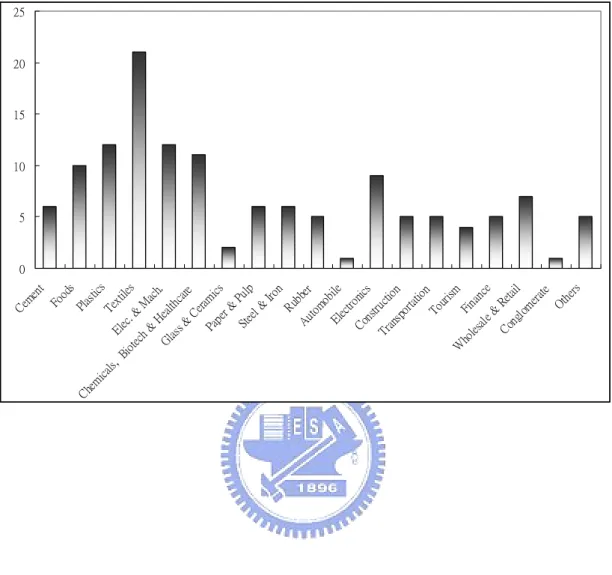
To be included in the sample, for a given month, a stock must satisfy certain criteria. First, its return over the previous 60 months must be available from the TEJ, and sufficient data must be available to calculate our variables, i.e. VaR and beta. Second, data must be available from the TEJ to calculate the book-to-market ratio as of December of the previous year. Finally, we include only securities defined by the TEJ as ordinary common shares. This screening process yields averages of 133

stocks per month. Therefore the returns for companies that are calculated are listed throughout the whole period. Figure 1 characterizes the industry distributions and gives a brief overview of the overall sample.

[Insert Figure 1 here]

3.2 Variable Definitions

For each stock and for each month, the following control variables are calculated.

3.2.1 Systematic risk (Beta)

Beta measures a stock’s volatility, i.e. the degree to which its price fluctuates in relation to the overall market. Beta is a key component of the capital asset pricing model (CAPM) and it expresses the fundamental tradeoff between minimizing risk and maximizing return. Follow Fama and French (1992), this paper first sorts all the stocks by size (i.e. the market value of equity) to determine the stocks’ quintile breakpoints. The reason why portfolios are formed according to their size is based on the evidence of Chan and Chen (1998) and others, who found that size differences may be attributed to a wide range of average returns and βs. Next, based on the stocks’ quintile breakpoints, this paper subdivides each size quintile into five portfolios on the basis of pre-ranking betas for all the stocks. This paper estimates the pre-ranking betas for five years of monthly returns ending in December of year t-1. After assigning each stock in the sample to one of five size quintiles and one of the pre-ranking beta quintiles, we then calculate the equally-weighted monthly returns of the resulting 25 portfolios2 for the next 12 months, from January of year t through December of year t. This procedure yields 108 post-ranking monthly returns for each of 25 portfolios from January 1996 to December 2004. Finally, this paper estimates the post-ranking betas by using a full sample of 108 post-ranking returns for each of the 25 portfolios, with the Taiwan stock value-weighted index serving as a proxy for the market. Following Allen and Cleary (1998), we estimate beta as the sum of the slopes in the regression of the returns on portfolios:

R_i,_t =α_i +β1,_iR_m,_t +β2,_iR_m,_t−1+ε_i,_t, （1）

2 The choice of using portfolios instead of individual shares is dictated by the evidence of Griffin (2002) that this is the way the sampling error is reduced. Additionally, using portfolios also facilitates a comparison with past studies in the field, as the majority of these studies use portfolios instead of individual stocks. Further advantages of using portfolios instead of individual firms in the regressions include the following: (1) A pooled sample of individual firms used in CSR analysis allows us to eliminate the potential threat posed by temporal and firm-specific effects in terms of biasing the results. (2) There is significantly less computational effort in using portfolios instead of individual stocks in the regression analysis.

where Ri,t is the monthly return on stock i in period t, αi is the intercept term,

is the monthly return on the TEJ value-weighted index in period t,

t m

R _, β is the _1,i

synchronous covariance coefficient, β is the lagged one-period coefficient, and 2,i t

i,

ε is the residual series from the cross-sectional regression.

The beta estimate used to rank stocks (the pre-ranking β) is calculated as follows:

i i i β1, β2,

β = + , （2） where β is the contemporaneous beta and1,i β is the lagged one-period beta. The 2,i

lag term allows for a delay in the information process, which may be prevalent for small stocks or those that are infrequently traded (Scholes and Williams, 1977).

3.2.2 Size

Size refers to the value of a company, that is, the market value of its outstanding shares. This figure is found by the natural logarithm of the market value of equity (by taking the stock price and multiplying it by the total number of shares outstanding).

3.2.3 Book-to-Market Equity (BE/ME)

Book-to-market equity (BE/ME) is the natural logarithm of the ratio of the book value of equity plus deferred taxes over the market value of equity, which involves accounting- and market-based variables. The book value of equity, in turn, is the value of a company’s assets expressed on the balance sheet. This number is defined as the difference between the book value of assets and the book value of liabilities. This paper uses a firm’s market equity at the end of December of the previous year to compute its BE/ME.

3.2.4 Value-at-Risk (VaR)

Value-at-Risk (VaR) has been widely promoted by the Bank for International Settlements (BIS) as well as central banks of all countries as a way of monitoring and managing market risk and as a basis for setting regulatory minimum capital standards.

The revised Basle Accord, implemented in January 1998, makes it mandatory for banks to use VaR as a basis for determining the amount of regulatory capital adequate for covering market risk. VaR measures the worst expected loss under normal market conditions over a specific time interval at a given confidence level. One of its definitions states: “VaR answers the question: How much can I lose with x% probability over a pre-set horizon?” Another way of expressing this is to state that VaR is the lowest quantile of the potential losses that can occur within a given portfolio during a specified time period.

There are three major decision variables required to estimate VaR: the confidence level, a target horizon, and an estimation model. In this paper, we use three confidence levels (90%, 95%, and 99%) to check the robustness of VaR as an explanatory variable for expected stock returns. The time horizon is 1 month and the estimation model is based on the historical simulation method. 3 The estimation model is also based on the lower tail of the actual empirical distribution. We use 60 monthly returns to estimate the mean, and the cut-off return at the 90%, 95%, and 99% confidence levels from the empirical distribution. The 1%, 5%, and 10% VaRs are measured by the first-lowest, third-lowest, and sixth-lowest observations from the 60 monthly returns.

Once we have the VaR measures for each stock, we rank and place them into 5 quintile portfolios. Portfolio 1 has the lowest VaR and portfolio 5 has the highest VaR. The portfolio formation procedure is very similar to Fama and French (1992), except that they update their portfolios annually, whereas we update ours on a monthly basis. The estimation period for VaR starts in January 1990 and extends through December 1995 and the test period extends from January 1996 to December

3 _{We also use EWMA and the Monte Carlo method to check the performance of our model. The}

2004. For example, in January 1996 we estimate VaR for each stock based on the return history from January 1990 to December 1995 and rank all the stocks according to the estimated VaRs. Then five equally-weighted portfolios are formed based on the VaR rank. We then calculate the one-month-ahead portfolio returns in January 1996. For the next month, by rolling over one month ahead, we re-estimate VaR for each stock, rank them based on the updated VaR, and form new portfolios. This procedure is repeated until December 2004 when we have no more data left. Therefore, we have 108 time series for the 5 equally-weighted portfolios based on their VaRs. In Figure 2-4, we graph the relationship between the 1%, 5% and 10% VaR levels and the average returns for the quintile portfolios. It is clear that the portfolios for the higher VaR tend to produce rates of return that are greater than the returns from the portfolios of lower VaR companies.

[Insert Figure 2-4 here]

4. Methodology and Models

4.1 Cross-Sectional Regression

This section tests whether the beta, size, BE/ME, 1% VaR, 5% VaR and 10% VaR can produce large and statistically significant cross-sectional variation in expected stock returns. This paper uses time series averages of the slopes from the month-by-month Fama-MacBeth (1973) (FM) regressions of the cross-section of realized average returns on Beta, Size, BE/ME, 1% VaR, 5% VaR, and 10% VaR. The average slopes provide standard FM tests for determining which explanatory variables on average have non-zero expected premiums during the January 1996 to

December 2004 period. Monthly cross-sectional regressions4 are run for the following econometric specifications:

Rj,t =ωt +γtBETAj,t +εj,t, (3) Rj,t =ωt +γtln(ME)j,t +εj,t, (4) Rj,t =ωt +γtln(BE/ME)j,t +εj,t, (5) R_j,t =ω_t +γ_tVaR1_j%_,t +ε_j,t, (6) R_j,t =ω_t +γ_tVaR5_j%_,t +ε_j,t, (7) R_j,t =ω_t +γ_tVaR10_j,t% +ε_j,t, (8) where j=1,2,…,t ( the number of firms in month t ), Rj,t is the realized average return

on stock j in month t, BETAj,t is the full-sample pre-ranking beta for firm j in month t,

and ln(ME)j,t is the natural logarithm of market equity for firm j in month t.

VaR(α)j,t is -1 times the maximum likely loss (VaR) for firm j in month t with the

loss probability level α=1%, 5%, and 10%, and εj,t is the residual series from the

cross-sectional regressions. The null hypothesis is the time series average of the monthly regression slopes, γt is zero, and statistical significance is established using

a standard t-test.

4.2 Inputs to the Time Series Regression 4.2.1 The Size – Book-to-Market Portfolios5

Following Fama and French (1993), this study forms six portfolios in order to

4 _{Cross-sectional regression analysis – a regression analysis where observations are measured at the}

same point in time or over the same time period, but which differ along another dimension. For example, an analyst may regress stock returns for different companies measured over the same period against differences in the companies’ fundamental variables for that period.

5 Portfolio analysis – a research method that ranks all stocks based on a certain variable, in order to consequently divide them into a given number of portfolios. For each portfolio an average value of the variable, on which the stocks were ranked and consequently divided into portfolios (the sorting variable), is calculated. The relationship between the average value of the sorting variable and the average portfolio returns (investigated in this study) is consequently examined.

examine the common risk factors in stock returns. The portfolios are formed yearly from a simple sorting of firms into two groups based on size and three groups based on the BE/ME. First, at the end of each year from 1996 to 2004, this study ranks all stocks in terms of size in order to allocate stocks into two groups, namely, small firms or big firms (S or B) according to the data for December of each previous year. The median size is used to split the stocks. Second, the stocks are also assigned to three BE/ME groups based on breakpoints for the bottom 30 percent (low, or L), the middle 40 percent (medium, or M), and the top 30 percent (high, or H) of the ranked values of the BE/ME for all stocks. Thus, six portfolios (S/L, S/M, S/H, B/L, B/M, and B/H) are finally constructed from the intersection of the two sizes and three BE/ME groups.

In a series of papers, Fama and French (1993, 1995, and 1996) documented the importance of RMRF, SMB, and HML. Fama and French used the excess return of the market over a risk-free return, i.e. RMRF, as a proxy for the market factor. RM was calculated as the return on the valued-weighted portfolio of the stocks in the six size-BE/ME portfolios plus the negative-BE stocks that were excluded from the portfolios. The risk-free rate, RF, was the one-month CD deposit rate from the Bank of Taiwan. The SMB was meant to mimic the risk factor in returns related to size, which is the difference, for each month, between the simple average of the returns on the three small-stock portfolios (S/L, S/M, and S/H) and the simple average of the returns on the three big-stock portfolios (B/L, B/M, and B/H). Thus, SMB (small minus big) is the difference between the returns on small- and big-stock portfolios with about the same weighted-average book-to-market equity. This difference should be largely free of the influence of BE/ME, focusing instead on the different return behaviors of small and big stocks

Similarly, HML (high minus low) is defined similarly and calculated based on the difference between the return on a portfolio of high-BE/ME stocks and the return on a portfolio of low-BE/ME stocks

HML= ((S/H+B/H)-(S/L+B/L))/2. (10) HVARL, similar to SMB, is defined as the equal-weighted average of the returns on the high-VaR stock portfolios minus the returns on the low-VaR stock portfolios.

4.2.2 The VaR - BE/ME Portfolios

In order to test the performance of VaR based on the 25 portfolios of Fama and French (1993), this study devises a factor, HVARL (high VaR minus low VaR), that is designed to mimic the risk factor in returns related to Value-at-Risk and is defined as the difference between the simple average returns on the high-VaR and low-VaR portfolios. The construction of a 5 percent VaR portfolio is similar to the construction of Fama and French’s size portfolios. In December of each year t from 1995 to 2004, this study ranks all stocks according to a 5 percent VaR. The median 5 percent VaR figure is used to divide the stocks into two groups — the high VaR and low VaR groups.

4.3 Main Model

This study performs a four-step analysis of the various factors (RMRF, HVARL, SMB, and HML) in explaining stock returns, and gradually examines the one- to four-factor models.

4.3.1 One-Factor Model

The one-factor regressions utilize RMRF, HVARL, SMB, and HML as explanatory variables to explain expected returns. They are in the following forms:

R(t)−RF(t)=a+b×[RM(t)−RF(t)]+u(t), (11)

R(t)−RF(t)=a+b×SMB+u(t), (13)

R(t)−RF(t)=a+b×HML+u(t), (14)

where RM is the value-weighted monthly percentage return on all the stocks in the 25 size-BE/ME portfolios, plus the negative –BE/ME stocks excluded from the 25 portfolios. RF is the one-month CD deposit rate from the Bank of Taiwan. SMB (small minus big), the return on the mimicking portfolio6 for the size factor in the stock returns, is the difference between the average of the returns on the three small-stock portfolios (S/L, S/M, and S/H) and the average of the returns on the three big-stock portfolios (B/L, B/M, and B/H). HML, the return on the mimicking portfolio for the size factor in the stock returns, is the difference between the average of the returns on the two high-BE/ME portfolios (S/H and B/H) and the two low-BE/ME portfolios (S/L and B/L). HVARL (high VaR minus low VaR) is the difference between the average of the returns on the high 5% VaR and low 5% VaR portfolios. Finally, is the error term of these 108 month-by-month cross-sectional regressions.

) (t

u

4.3.2 Two-Factor Model

The two-factor regressions employ RM-RF along with either HVARL, SMB, or HML as explanatory variables to explain expected returns. They are in the following forms: R(t)−RF(t)=a+b×[RM(t)−RF(t)]+c×HVARL+u(t), (15) R(t)−RF(t)=a+b×[RM(t)−RF(t)]+c×SMB+u(t), (16) R(t)−RF(t)=a+b×[RM(t)−RF(t)]+c×HML+u(t). (17) 4.3.3 Three-Factor Model

6 Mimicking portfolios – zero-investment portfolios that are sensitive to a potential risk factor, proxied by the variable on which they were created. More specifically, a mimicking portfolio is constructed by buying assets with a high value of the sorting variable (size or BE/ME in our case) and selling assets with a low value of the factor at the same time, which in effect maximizes the portfolio risk with respect to the factor proxied by the sorting variable.

The three-factor model suggested by Fama and French (1993) provides an alternative to the CAPM for the estimation of expected returns. In this model, two additional factors are included to explain excess return; size and the book-to-market ratio.7 The Fama and French model is of primary interest to us as one of the objectives of the paper is to assess its implications for the investor’s investment decision. The explanatory variables in the time series regressions include not only the returns on a market portfolio of stocks but also the mimicking portfolio returns for size and book-to-market:

R(t)−RF(t)=a+b×[RM(t)−R(t)]+c×SMB+d×HML+u(t). (18)

4.3.4 Four-Factor Model

The fourth model, the four-factor model, adds another risk factor, i.e. HVARL, to the three-factor model. The risk factor is a mimicking portfolio that follows Bali and Cakici (2004): ) ( )] ( ) ( [ ) ( ) (t RF t a b RM t RF t c SMB d HML e HVARL u t R − = + × − + × + × + × + . (19) 7

Markowitz (1999) argues that the existence of these anomalies can be due to several sources but can broadly be grouped into three categories. He states, “The first possibility is that these anomalies arise because the asset-pricing model is not capturing a component of systematic risk, which these firm characteristics may be correlated with. The second set of explanations are behavioral, suggesting that these anomalies arise because investors care about certain firm attributes, or that investors act irrationally to information, or have psychological biases in their interpretation of information, all of which may induce an apparent relation between average returns and these firm characteristics. Finally, the third set of explanations arises from flawed methodology, such as biases in computing returns from firm survivorship or microstructure effects, as well as other statistical errors.” (p.1)

5. Empirical Results

5.1 VaR and Cross–Sectional Regression

To begin our analysis, we present the results of the Fama and MacBeth regressions of excess returns on characteristics that are best known to be associated with expected returns, namely, the beta, firm size, BE/ME, and VaR (1%, 5%, and10%) variables.

[Insert Table 1 here]

Table 1 presents the time series average value of γ_t, the t-statistics, and the time series averages of the determination coefficient ( 2

R ) over the 108 months in the

sample. The t-statistics shown in the parentheses are the time series average values of γt divided by the corresponding time-series standard errors. As can be seen

from the estimated slopes of beta, ln(ME) and ln(BE/ME) are both highly significant at the 1% level. The average slopes provide standard FM tests for determining which explanatory variables had, on average, nonzero expected return premiums during the January 1996 to December 2004 period. As expected, there is a strong relationship between the realized stock returns and beta. The empirical evidence shows that, the greater the sensitivity of the asset return, the greater the realized return. However, the average slope for the monthly regressions of the realized returns and size, ln(Size), is positive and about 0.49, with a t-statistic of 34.81. We think that size may be related to profitability. On average, the profitability of larger-cap stocks in the Taiwan stock market is better than that of smaller-cap stocks. This result also shows that, for a firm with larger capitalization, the performance seems much better than for the small firm from the viewpoint of the cross-sectional regressions. The average slope based on the univariate regressions of the monthly return on ln(BE/ME)

is about 0.94, with a t-statistic of 17.36. This positive relationship indicates that it is possible that the risk captured by BE/ME is the relatively distressed factor of Chan and Chen (1991). They postulate that the earning prospects of firms are associated with a risk factor in the returns. Firms that the market judges to have poor prospects, signaled here by low stock prices and high BE/ME ratios, have higher expected returns (they are penalized with higher costs of capital) than firms with strong prospects. It is also possible that BE/ME only captures the unraveling of irrational market whims regarding the prospects of firms. This accords with the view put forward by Fama and French (1992) that BE/ME has a stronger role in explaining average stock returns than size. Furthermore, as we move to a lower significance level (higher confidence level), the VaR estimation becomes more important in explaining the cross-sectional average stock returns. We can see that the Var(α) are significant when the α are 1% and 5%. The results of the positive coefficients of VaR indicate that the greater a stock’s potential fall in value, the higher the expected return should be.

5.2 VaR and Time-Series Variation of Expected Returns

In time-series regressions, the slopes and 2

R values are direct evidence as to

whether different risk factors capture a common variation in stock returns. This study examines the explanatory power of stock market factors.

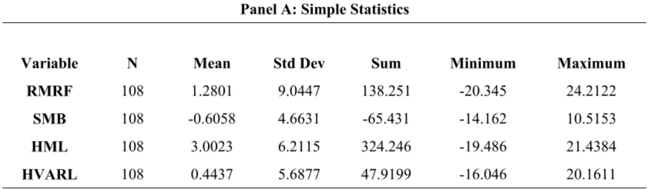
[Insert Table 2 here]

Table 2 of Panel A shows the simple statistics of RMRF, SMB, HML and HVARL. The average value of the market risk premium is 1.28% per month. This study also calculates the correlations between RMRF, SMB, HML and HVARL. Table 2 of Panel B presents the correlation coefficients for the factors used. The last

row shows that HVARL is positively correlated with RMRF and SMB, whereas it is negatively correlated with HML. A notable point is that the positive relationship between HVARL and SMB is much stronger than the negative relationship between HVARL and HML.

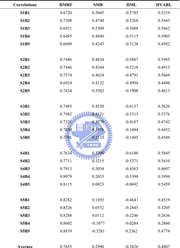
To compare the relative performances of HVARL, RMRF, SMB and HML, this study calculates the correlations between the returns for the 25 portfolios of Fama and French (1993) and the various factors:

[Insert Table 3 here]

Table 3 shows that, not surprisingly, the excess return on the market portfolio of stocks, RMRF, captures more common variation in stock returns, on average, than HVARL, HML and SMB. The average correlation between the returns for the 25 portfolios and RMRF is 0.7655, whereas the average correlation between HVARL and the monthly returns on the 25 portfolios is 0.4807. Furthermore, the average correlation is 0.2990 for SMB, and -0.3826 for HML. Clearly, HVARL, as a single factor, is superior to SMB and HML in explaining the time-series variation in stock returns.

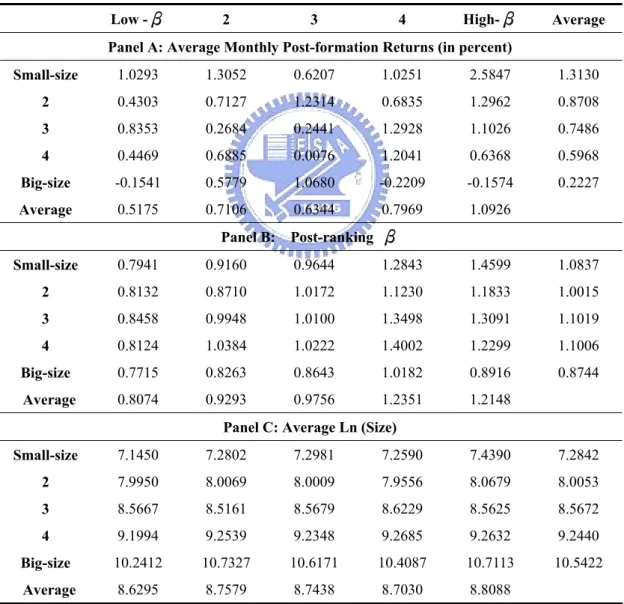
5.3 Properties of Portfolios Formed Based on Size and Pre-ranking β

Fama and French (1992) found that after controlling for the size and book-to-market effects, beta seemed to have no power to explain the average returns on a security. This finding is an important challenge to the notion of a rational market, since it seems to imply that a factor that should affect return, namely, systematic risk, does not seem to matter.

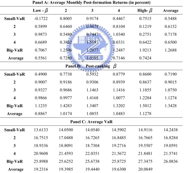
The average row of Panel B of Table 4 shows that the portfolio beta of each beta group averaged across the 5 different-sized portfolios steadily increases from 0.81 to 1.21. The average row in Panel C shows that the average portfolio size within each beta group is almost identical, ranging from 8.63 to 8.81. This allows us to interpret Panel A as a test of the net effect of beta on average returns holding size fixed. Panel A of Table 4 clearly shows that, for the period 1996-2004, average returns are not positively related to beta. The highest-beta portfolios do not have the highest returns, and it occurs in the fourth-beta portfolios. The results do not support the central prediction of the CAPM, because average stock returns are not positively related to the market beta at the portfolio level. The CAPM insight is that volatility arising from specific events (called specific or idiosyncratic risk) can be eliminated in a diversified portfolio, and that investors will not be paid for bearing these risks with extra returns. This result will support us as we continue to further discuss the three- and four-factor models. We should note that average monthly post-formation returns seem to be negatively correlated with firm size. The smallest size quintile, on average, has the highest average return (1.31% per month) and the biggest size quintile has the lowest average return (0.22% per month).

5.4 Properties of Portfolios Formed on VaR and Pre-ranking β

[Insert Table 5 here]

Table 5 of Panel A reports that when common stock portfolios are formed on 5% VaR, the average stock returns are positively related to VaR. Going from the lowest 5% VaR quintile to the highest 5% VaR quintile, the average stock returns from VaR portfolios increase from 0.55% per month to 1.27% per month monotonically. This result supports our argument to the effect that if investors are more averse to the risk

of losses on the downside than of gains on the upside, i.e. a higher VaR, investors ought to demand greater compensation. Furthermore, we can see that the greatest average monthly post-formation return is about 1.92% and not surprisingly is apparent in the highest VaR-BE/ME group. However, the average monthly post-formation returns are not similar within the sameβ quintile. For the smallest 5% VaR quintile, the highest β does not have the largest stock returns. Beta seems to have much less power to explain the average stock returns after controlling for the 5% VaR and book-to-market effects. These results inform us that the more a stock can potentially fall in value, the higher should be the expected return.

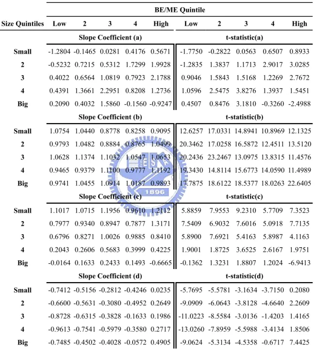
5.5 Main Model Results: Factor Models

[Insert Table 6 here]

Table 6 shows, not surprisingly, the excess return on the market portfolio of stocks. RMRF captures a more common variation in stock returns than SMB, HML, and HVARL. As presented in Panel A of Table 6, the coefficients of RMRF are in the range of 0.78 to 1.17, and the t statistics are in the range of 8.77 to 19.46. The

2

R values are extremely high, but the important fact is that the market leaves much variation in stock returns that might be explained by other factors. The only _R 2

value near 0.8 is related to the big-stock high-BE/ME portfolios. For small-stock and low-BE/ME portfolios, the _{R are less than 0.6 or 0.5, respectively. Panel B of} 2

Table 6 indicates that HVARL, even if used alone, captures substantial time-series variation in stock returns. The slopes on HVARL range from 0.45 to 1.38, and their t-statistics are in the range of 2.81 to 7.69. We should note that 20 of the 25 _R 2

values are above 0.20. Panel C of Table 6 shows that SMB, the mimicking return for the size factor, has less power than HVARL in terms of explaining stock returns.

The _{R values in Panel B are greater than those in Panel C. It should be noted that} 2

both HVARL and SMB have little power for the portfolios in the big-size quintile. Specifically, the _{R values for HVARL are in the range of 0.08 to 0.23, whereas the} 2

corresponding figures for SMB range from 0.00 to 0.11. As expected, on average, the slopes for SMB are related to size. In every BE/ME quintile in Panel C, the slopes for SMB decrease monotonically from smaller- to bigger-size quintiles. We can see an interesting result in that smaller-size quintiles seem to capture more variations in terms of _{R values. Panel D of Table 6 points out that for HML,} 2

when used alone, the slopes in relation to HML increase monotonically from the strong negative values for the smaller- to bigger-size quintiles. Not surprisingly, the slopes for HML are systematically related to BE/ME. The _{R values for the} 2

small-stock small-BE/ME portfolios capture more of the variations in stock returns and range from 0.22 to 0.38. This result accords with the intuition that the stocks with lower BE/ME ratios are less risky and so lower stock returns are required.

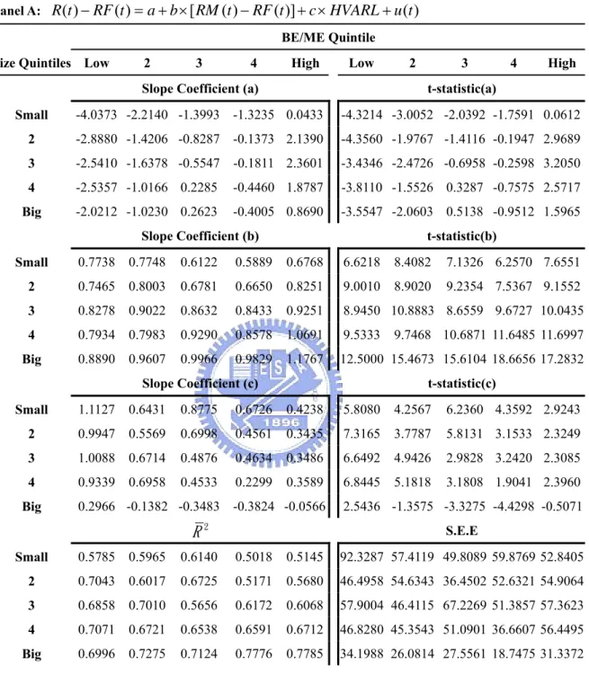
[Insert Table 7 here]

Table 7 shows two-factor models in which monthly returns on 25 portfolios are regressed on RMRF along with SMB, HML and HVARL. Panel A of Table 7 displays the slope coefficients for RMRF and HVARL, their t-statistics, _{R values} 2

and the standard error values of estimates (SEE). All of the slopes of RMRF are statistically significant at the 5% level. The _{R values are in the range of 0.50 to} 2

0.78. Panel B of Table 7 presents very similar results for RMRF and SMB. The market βs for stocks are all significant according to the t-statistics. On average, 22 of the 25 slope coefficients for HVARL are statistically different from 0. The _R 2

along with RMRF, capture substantial time-series variation in stock returns. Panel C of Table 7 indicates that only 3 of the 25 coefficients for HML are statistically insignificant, and the _{R values range from 0.54 to 0.90. Similar to Table 6, the} 2

slope coefficients for SMB and HML are related to the size and BE/ME factors, respectively. In every BE/ME quintile, on average, the SMB slopes decrease monotonically from small- to big-size quintiles. For every size quintile for stocks, the HML slopes increase monotonically from strong negative values for the lowest-BE/ME quintile to strong positive values for the highest-BE/ME quintile.

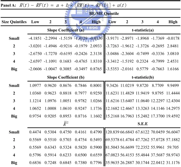
[Insert Table 8 here]

Table 8 presents estimates from the three-factor model in which the excess returns on 25 portfolios are regressed on RMRF, SMB and HML. Table 8 demonstrates that most of the coefficients for the three Fama-French factors (RMRF, SMB and HML) are highly significant. The lower BE/ME quintile and bigger size quintile portfolios capture between 70% and 90% of the variations in terms of the _R 2

values. However, the higher BE/ME quintile and smaller size quintile seem to leave 30%-40% of variations that cannot be explained by Fama and French’s three-factor model. Furthermore, the results indicate that, when controlling for the BE/ME effect, the SMB factor loading is highly significant. What is initially surprising, however, is the fact that SMB seems to work in a reverse manner than what would be expected, i.e. small firms have on average higher returns than big firms. This can be seen by looking at the coefficients for SMB, which go from positive to negative when moving from small stock portfolios to big stock portfolios and after taking into account the fact that the size premium is negative during our sample period. On the other hand, when controlling for size, the HML factor clearly captures the higher returns for the

high BE/ME portfolios as compared to the low BE/ME stocks. Subsequently, we will continue to see if another factor — the VaR — can enhance and capture the variations.

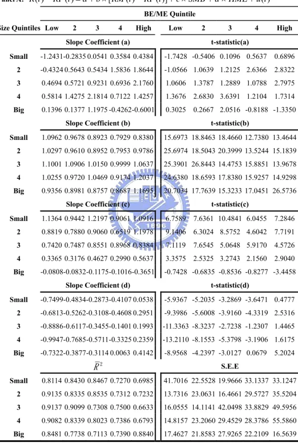
[Insert Table 9 here]

Table 9 presents the parameter estimates, t-statistics, _{R values, and standard} 2

errors of estimate (S.E.E) from the time series regressions of excess stock returns on RMRF, SMB, HML and HVARL. As shown in Table 9, the slope coefficients for the market factor, RMRF, are highly significant. Most of the slope coefficients for SMB and HML factor are also significant. A notable point is that, for the lowest size-quintile, none of HVARL slopes are significant. Only 8 of 25 HVARL slopes are significant. The _{R values of the four-factor model are greater than those of} 2

the three-factor model. When viewed at the portfolio level, these empirical results show that the VaR factor plays an important role in firms especially with larger capitalization. This could be the reason why either the concept of VaR is not very familiar to individual investors since they are the major participants in Taiwan’s stock market or else larger companies always pay much attention to VaR in order to control for downside risk. However, the New Basle II Accord will be implemented at the end of 2006, and so we think VaR will play an increasingly important role in the future. Therefore, this could perhaps be tested and verified by further research.

6. Conclusions and Comments

By focusing on downside risk as an alternative measure of risk measured by VaR, this paper investigates whether the new VaR factor plays an important role in explaining Taiwan’s stock returns from January 1996 to December 2004. The empirical results

do not support the central prediction of the CAPM because average stock returns are not positively related to the market beta at the portfolio level. From the cross-sectional regressions in a Fama and French (1992) asset pricing framework, we can find that, in addition to market betas, idiosyncratic factors, such as firm size, book value of equity to market value of equity, 1% VaR and 5% VaR, are related to the return at the individual stock level. In particular, the BE/ME factor captures most of the variations in average realized stock returns in terms of _{R . From the time series} 2

regressions we investigate models with factors ranging from one to four to test the empirical performance at the portfolio level. From the results, which are based on 25 size/book-to-market portfolios of Fama and French (1993) and follow Bali and Cakici (2004), we find that the HVARL factor can also help to explain the variation in the stock market, especially for the larger companies in Taiwan’s stock market. One direction for future research could explore whether expected returns are related to a stock’s sensitivities to fluctuations in other aspects of VaR. Another point is that since expected average returns seem to be explained by the four-factor risk return relationship, it would be interesting to analyze whether it is the time variation in expected premiums or the time variation in the factor sensitivities that capture most of the predicted variation in the expected returns.

References

Allen D.E., and F. Cleary, 1998, Determinants of the cross-section of stock returns in the Malaysian stock market, International Review of Financial Analysis 7, 253-275.

Ball, R., 1978, Anomalies in relationships between securities’ yields and yield-surrogates, Journal of Financial Economics 6, 103-126.

Bali, T. G.. and N. Cakici, 2004, Value at risk and expected stock returns, Financial

Analysts Journal 60, 57-73.

Banz, R. W., 1981, The relationship between return and market value of common stocks, Journal of Financial Economics 9, 3-18.

Basu, S., 1977, The investment performance of common stocks in relation to their price-earnings ratios: A test of the efficient market hypothesis, Journal of Finance 32, 663–82.

Berk, J., 1995, A critique of size-related anomalies, Review of Financial Studies 8, 275-286.

Black, F., 1972, Capital market equilibrium with restricted borrowing, Journal of

Business 45, 444-455.

Black, F., M.C. Jensen, and M. Scholes, 1972, The capital asset pricing model: Some empirical tests, in: M. Jensen, ed., Studies in the Theory of Capital Markets (Praeger).

Black, F., 1993, Beta and return, Journal of Portfolio Management 20, 8-18.

Campbell, John Y., Martin Lettau, Burton G. Malkiel, and Yexiao Xu, 2001, Have individual stocks become more volatile? An empirical exploration of idiosyncratic risk, Journal of Finance 56, 1-43.

Chan, L., Y. Hamao, and J. Lakonishok, 1991, Fundamentals and stock returns in Japan, Journal of Finance 46, 1739-1764.

Chan, K. C., N. Chen, and D. Hsieh, 1985, An exploratory investigation of the firm size effect, Journal of Financial Economics 14, 451-471.

Chan, K. C., and Nai-Fu Chen, 1991, Structural and return characteristics of small and large firms, Journal of Finance 46, 1467-1484.

Chen, Nai-Fu and Feng Zhang, 1998, Risk and return of value stocks, Journal of

Business 4, 501-535.

Chui, Andy C.W., and K.C. John Wei, 1998, Book-to-market, firm size, and the turn-of-the-year effect: Evidence from Pacific-Basin emerging markets,

Pacific-Basin Finance Journal, 6, 275-293.

Clare, A.D., R. Priestley, and S.H. Thomas, 1998, Reports of beta’s death are premature: Evidence from the UK, Journal of Banking and Finance 22, 1207-1229.

Daniel, K., and S. Titman, 1997, Evidence on the characteristics of cross-sectional variation in stock returns, Journal of Finance 52, 1-33.

Daniel, K., S. Titman, and K.C. John Wei, 2001, Explaining the cross-section of stock returns in Japan: Factors or characteristics? Journal of Finance 56, 743-766. Duffee, Gregory R., 1995, Stock returns and volatility: A firm-level analysis, Journal

of Financial Economics 37, 399-420.

Engle R. F., and S. Manganelli, 1999, CAViaR: Conditional autoregressive Value at Risk by regression quantiles, Journal of Business and Economic Statistics 22. Fama, E. F., and J. MacBeth, 1973, Risk, return and equilibrium: Empirical tests,

Journal of Political Economy 81, 607-636.

Fama, E. F., and K. French, 1992, The cross-section of expected stock returns,

Journal of Finance 47, 427-465.

____, 1993, Common risk factors in the returns on stocks and bonds, Journal of

____, 1995, Size and book-to-market factors in earnings and returns, Journal of

Finance 50, 131-155.

____, 1996, The CAPM is wanted, dead or alive, Journal of Finance 51, 1947-1958. Gibbons, M. R., 1982, Multivariate tests of financial models: A new approach,

Journal of Financial Economics 10, 3-27.

Heston, Steven L., K. Geert Rouwenhorst, and Roberto E. Wessels, 1999, The role of beta and size in the cross-section of European stock returns, European Financial

Management 5, 9-27.

Jansen, Paul F. G. and Willem F. C. Verschoor, 2004, A note on transition stock return behavior, Applied Economics Letters 11, 11-13.

Kim, D., 1997, A reexamination of firm size, book-to-market, and earnings price in the cross-section of expected stock returns, Journal of Financial and Quantitative

Analysis 32, 463-489.

Kothari, S. P., J. Shanken, and R. G. Sloan, 1995, Another look at the cross-section of expected stock returns, Journal of Finance 50, 185-224.

Lakonishok, J., A. Shleifer, and R. Vishny, 1994, Contrarian investment, extrapolation, and risk, Journal of Finance 49, 1541-1578.

Lintner, John, 1965, The valuation of risk assets and the selection of risky investments in stock portfolios and capital budgets, Review of Economics and Statistics 47, 13-37.

Markowitz, H., 1959, Portfolio Selection: Efficient Diversification of Investments (Wiley, New York).

Miller, Merton H., and Myron Scholes, 1972, Rate of return in relation to risk: A reexamination of some recent findings, in Michael C. Jensen, ed., Studies in the

Penman, S. H., 1991, An evaluation of the accounting rate of return, Journal of

Accounting, Auditing, and Finance 6, 233-255.

Reinganum, M. R., 1981, Misspecification of capital asset pricing: Empirical anomalies based on earnings yields and market values, Journal of Financial

Economics 9, 19-46.

RiskMetrics, 1996, Technical Document, Morgan Guaranty Trust Company of New York.

Roll, R., 1995, An empirical survey of Indonesian equities 1985-1992, Pacific-Basin

Finance Journal 3, 159-192.

Rosenberg, B., K. Reid, and R. Lanstein, 1985, Persuasive evidence of market inefficiency, Journal of Portfolio Management, 11, 9-17.

Ross, Stephen A., 1976, The arbitrage theory of capital asset pricing, Journal of

Economic Theory 13, 341-360.

Rouwenhorst, K. Geert, 1999, Local return factors and turnover in emerging stock markets, Journal of Finance 54, 1439-1464.

Sharpe, William F., 1964, Capital asset prices: A theory of market equilibrium under conditions of risk, Journal of Finance 19, 425-442.

Stambaugh, R.F., 1982, On the exclusion of assets from tests of the two-parameter model: A sensitivity analysis, Journal of Financial Economics 10, 237-268.

Stattman, D., 1980, Book values and stock returns, The Chicago MBA: A Journal of

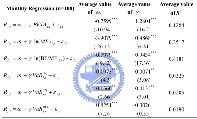
Table 1: Cross-Sectional Regressions of Stock Returns on Beta, Size, BE/ME, and VaR

This table reports the time-series average of the month-by-month regression slopes from January 1996 to December 2004. The dependent variables are the monthly average returns on individual stocks. The independent variables include beta, firm size, the book-to-market ratio (BE/ME), and VaR(α), where α=1%, 5%, and 10%. The betas that correspond to the portfolio they belong to are assigned to individual stocks. The size is the natural log of the market value. The BE/ME is the natural log of the book-to-market value. The VaR is calculated using the historical simulation method. The t-statistic reported in the parentheses is the average slope divided by its time-series standard error.

Monthly Regression (n=108) Average value of ω_t Average value of γ_t Average value of 2 R t j t j t t t j BETA R , =ω +γ , +ε , -0.7599 (-10.94) *** _1.2601 (16.2) *** 0.1284 t j t j t t t j ME R , =ω +γ ln( ) , +ε , -3.9079 (-26.13) *** _0.4868 (34.81) *** 0.2517 t j t j t t t j R , =ω +γ ln(BE/ME , )+ε , -0.7979 (-9.82) *** _0.9434 (17.36) *** 0.4181 t j t j t t t j VaR R _, =ω +γ 1%_, +ε _, 0.1973 (4.3) *** _0.0071 (3.08) ** 0.0325 t j t j t t t j VaR R _, =ω +γ 5%_, +ε _, 0.1560 (2.66) ** _0.0135 (3.01) ** 0.0205 t j t j t t t j VaR R _, =ω +γ 10_,% +ε _, 0.4251 (7.24) *** _-0.0020 (0.35) 0.0190

Note: ***, **, * denotes significantly different from zero at the 0.01, 0.05, and 0.10-levels, respectively.