基於影像處理方法之心電圖小波係數研究

全文

(1)國立交通大學電機與控制工程學系碩士論文基於影像處理方法之心電圖小波係數研究. Investigation of Wavelet Coefficient of Electrocardiograph based on Image Processing Method. 研究生：林國祥指導教授：羅佩禎博士. 中華民國九十七年七月.

(2) 基於影像處理方法之心電圖小波係數研究 Investigation of Wavelet Coefficient of Electrocardiograph based on Image Processing Method. Student：Buwono Lembono. 研究生：林國祥. Advisor：Dr. Pei-Chen Lo. 指導教授：羅佩禎博士國. 立. 交. 通. 大. 學. 電機與控制工程學系碩士論文 A Thesis Submitted to Department of Electrical and Control Engineering College of Electrical and Computer Engineering National Chiao Tung University In Partial Fulfillment of the Requirements For the Degree of Master In Electrical and Control Engineering July 2008 Hsinchu, Taiwan, Republic of China. 中華民國九十七年七月.

(3) 基於影像處理方法之心電圖小波係數研究. 研究生：林國祥. 指導教授：羅佩禎博士. 國立交通大學電機與控制工程學系. 摘要本研究的目的在於以不同的量化方法來分析禪坐心電訊號(ECG)的小波係數(continuous wavelet coefficients, CWT)。研究中所採用的量化的方法包括：不變矩分析 (invariant-moment analysis) 、奇異值分解 (singular value decomposition, SVD) 、相關係數 (correlation coefficient) 以及變異數分析 (ANOVA)。本研究的實驗受測者共有 17 位，實驗組是 8 位有禪坐經驗的受測者，而控制組是 9 位沒有禪坐經驗的受測者，兩組受測者的年齡相近。研究結果顯示，控制組的 7 個不變矩數值下降，而實驗組則是上升。在相關係數分析的部份，除了控制組的一位受測者之外，其餘受測者的心電訊號小波係數的主成份，在不同狀態下皆呈現很高的相關性。變異數分析的結果則顯示，比起實驗組，控制組的心電訊號小波係數在不同狀態下的差異較為顯著。因此，由以上結果可以得知實驗組的心電訊號波形較控制組穩定。. i.

(4) Investigation of Wavelet Coefficient of Electrocardiograph based on Image Processing Method. Student : Buwono Lembono. Advisor :Dr. Pei-Chen Lo. Institute of Electrical and Control Engineering National Chiao-Tung University. Abstract The aim of this research was to quantify the continuous wavelet coefficients (CWT) of raw ECG data. Several methods employed in this thesis included invariant-moment analysis, singular value decomposition (SVD), correlation coefficient, and analysis of variance (ANOVA). This study included 17 subjects, 8 experimental subjects with Zen-meditation experience and 9 control subjects in the same age range, yet, without any meditation experience. According to our results, the seven invariant moment values in control group tended to decrease, while the experimental group showed the tendency of increase. SVD analysis gives us another perspective. The correlation coefficients between major components of both groups showed a high value of correlation, although one result from the control group was considered to be moderately correlated. In ANOVA, differences appeared to be more significant in the control group than the experimental group. Thus, we may preliminarily suggest that ECG waveform patterns of experimental group behave more stably than those of control group in certain condition. ii.

(5) Acknowledgements. I would like to express my profound gratitude to my advisor Dr. Pei-Chen Lo for her invaluable source of support, guidance and direction throughout the course of this research, and I have benefited enormously from his wisdom during my time of studying in National Chiao Tung University. I would like to thank my Biomedical Signal Processing Laboratory leader and senior, Shr-Da Wu, for his support, suggestions and help throughout my two years study. I would like to thank the National Chiao Tung University for the scholarship and financial support so that I can continue and finished my master degree. I would like to express my gratitude to Dr. Sheng-Fuu Lin and Dr. Guo-Rui Lin for kindly serving as the members of this thesis committee, and appreciate their constructive comments and suggestions. Moreover, I want to express my appreciation to my parents for their concern and unlimited support. Also thank for brother and all my friends (Wono, Irfan, Agus, Dedy, Martin, Roiki, Rosalinda, Oh Chee Way, Suyanti, Donna) and many others that cannot be mentioned one by one. Least but not last I want to present this thesis for Jesus Christ (without Him I will not able to finished my study and my thesis).. Buwono Lembono National Chiao Tung University July 2008. iii.

(6) Contents 中文摘要 .......................................................................................................................... i Abstract ........................................................................................................................... ii Acknowledgements.................................................................................................... iii Contents.......................................................................................................................... iv List of Tables ................................................................................................................ vi List of Figures ............................................................................................................. vii 1. Introduction .............................................................................................................. 1 1.1 Background and Motivation................................................................................. 1 1.2 Aims of this Work.................................................................................................. 3 1.3 Organization of this Thesis................................................................................... 3. 2. Theories and Methods ......................................................................................... 5 2.1 Introduction to ECG and Respiratory Signals.................................................... 5 2.1.1 Introduction to ECG .................................................................................... 5 2.1.2 Introduction to Respiratory Signals ........................................................... 8 2.2 Wavelet Transformation........................................................................................ 9 2.3 Quantification of Wavelet Coefficients .............................................................. 13 2.3.1 Hu’s Invariant Moments............................................................................. 13 2.3.2 Singular Value Decomposition ..................................................................14 2.3.3 Correlation Coefficient............................................................................... 15 2.3.4 Analysis of Variance (ANOVA) ................................................................16. 3. Experiment and Signal Analysis ....................................................................20 3.1 Experimental Setup and Protocol .......................................................................20 3.1.1 Measurement of ECG signal......................................................................21 iv.

(7) 3.1.2 Measurement of Respiratory Signal.......................................................... 22 3.2 Wavelet Transform of ECG Signal .....................................................................23 3.3 Quantification of Wavelet Coefficients .............................................................. 26 3.3.1 Invariant Moments Analysis ......................................................................28 3.3.2 SVD Integrated with Correlation Coefficient .......................................... 29 3.3.3 Analysis of Variance (ANOVA) Procedure .............................................. 32. 4. Results ........................................................................................................................35 4.1 Results of Invariant Moments Analysis ............................................................. 35 4.1.1 Comparison of Invariant Moments at Different Respiration Rates .......36 4.1.2 Comparison of Invariant Moments in Different Session ........................ 38 4.2 Results of Singular Value Decomposition Analysis.......................................... 42 4.3 Results of ANOVA ............................................................................................... 46. 5. Conclusion and Discussion ...............................................................................53 5.1 Preliminary Conclusion ....................................................................................... 53 5.2 Future Work .......................................................................................................... 54. References...................................................................................................................... 55 Appendix A. Detection of ECG R Peak and Respiratory Peak ...........59 A.1 R-Peak Detection................................................................................................. 59 A.2 Respiratory Peak Detection and Respiration Rate ........................................... 62. v.

(8) List of Tables 2.1. One-way ANOVA typical data ............................................................................... 17. 2.2. ANOVA table ........................................................................................................... 19. 3.1. Subjects of experimental and control groups........................................................ 21. 4.1. Mean values of three respiration rate ranges analyzed for the experimental and control group on session 1 and 2 .....................................................................35. 4.2 4.3. Weighted percentage of each eigenvalues............................................................. 43 Correlation-coefficient analysis of the first eigenvector of ECG-complex CWT-coefficient maps ............................................................................................ 45. vi.

(9) List of Figures 2.1 Cardiac conduction system ........................................................................................ 6 2.2 The typical wave complex of ECG ...........................................................................7 2.3 Mechanics of inhalation (inspiration) and exhalation (expiration)........................ 8 2.4 Morlet mother wavelet (real part) ........................................................................... 11 2.5 Illustration of constructing continuous wavelet transforms..................................12 2.6 (a) Original ECG signal, (b) Morlet based scalogram of (a) ................................12 2.7 Singular value decomposition .................................................................................15 3.1 Experimental protocol ..............................................................................................20 3.2 The physiological signal recording system ............................................................22 3.3 (a) LeadⅠconfiguration of bipolar limb leads, (b) Disposable ECG electrode....................................................................................................................22 3.4 Piezo-electric respiratory transducer.......................................................................23 3.5 Respiratory signal .....................................................................................................23 3.6 Flow chart of continuous wavelet transforms ........................................................24 3.7 The wavelet scalogram of a control group subject during session 1 ...................25 3.8 Flowchart of CWT quantification strategy.............................................................26 3.9 (a)Extraction of ECG complexes based on R peaks, (b) one ECG complex wavelet coefficient template...................................................................................27 3.10 Flowchart of Hu’s invariant moments algorithm.................................................28 3.11 (a) Wavelet coefficient of one subject from control group, (b) Seven. vii.

(10) invariant moments values......................................................................................29 3.12 Flowchart of SVD and correlation coefficient algorithm ...................................30 3.13 Illustration of SVD extraction algorithm..............................................................31 3.14 Illustration of ANOVA algorithm..........................................................................32 3.15 Flowchart of ANOVA algorithm ...........................................................................33 3.16 P-value map as result of ANOVA .........................................................................34 4.1 Result of Control Group Invariant moments S1 and S2 .......................................36 4.2 Result of Experimental Group Invariant moments S1 and S2 .............................37 4.3 Seven invariant moments from S1 to S2 for respiration rate (a) A: slow breathing, (b) B: normal breathing, and (c) C: fast breathing (control group) ..................... 39 4.4 Seven invariant moments from S1 to S2 for respiration rate (a) A: slow breathing, (b) B: normal breathing, and (c) C: fast breathing (experimental group)........................................................................................................................40 4.5 Second Order Moments in (a) Control Group and (b) Experimental Group ......41 4.6 Singular Value Decomposition (a) a Control Group Subject and (b) an Experimental Group Subject (from top: CWT-coefficient map, the first and the second eigenvector)............................................................................................42 4.7 (a) Control Subject’s and (b) Experimental Subject’s 1st eigenvector and their correlation coefficient between respiration ranges ......................................44 4.8 Control subject 1st eigenvector between S1 and S2 slow breathing ....................46 4.9 ANOVA analysis for Control Group (intra session, different rates of respiration)................................................................................................................47 4.10 ANOVA analysis for Experimental Group (intra session, different rates of respiration)................................................................................................................48 4.11 ANOVA analysis for Control Group (inter session, samedifferent rates of respiration)..............................................................................................................50 viii.

(11) 4.12 ANOVA analysis for Experimental Group (inter session, same rates of respiration) ..............................................................................................................51 A.1 Flow chart of R peak detection...............................................................................59 A.2 The raw ECG and preprocessed ECG....................................................................61 A.3 R peak detection by threshold ................................................................................61 A.4 Flow chart of Respiratory peak detection and respiration rate............................62. ix.

(12) Chapter 1 Introduction 1.1 Background and Motivation The applications of digital signal processing methods play important role in processing, quantifying, analyzing, and identifying biomedical signals such as electrocardiogram (ECG or EKG), electroencephalogram (EEG) and electromyogram (EMG) signals. A lot of researches and studies focused on feature extraction and pattern recognition in the biomedical signal processing have achieved tremendous contributions to the clinical field today. Classical approach using time-domain method on quantitative electrocardiology involves measuring amplitude and duration of ECG waves. This method is not always feasible to adequately describe important features of the ECG signal. On the other hand, some researches reported that ECG abnormalities caused by cardiac diseases could not be explored by time-domain methods. Techniques based on frequency domain or time-frequency domain were found to be useful [1], [2]. The frequency components of a signal can be obtained by using different methods, including the Fourier transformation and the autoregressive and/or moving-average method. Strictly speaking, ECG signals are not exactly periodic in spite of the rhythmic activity of heart beating. To analyze such kind of ‘pseudo-periodic’ behavior, frequency component alone is not sufficient for characterizing ECG signals. Fourier transformation loses the time information after transforming time domain signal to frequency domain. Moreover, it does not give insight into time-dependent variation of frequency components. 1.

(13) The frequency component of the ECG involves multi-frequency complex evolving with time. For example, QRS complex contains sharp transient with higher-frequency spectrum, whereas the T wave is characterized by slowly varying pattern. Therefore it is essential to obtain “time-based” information when a particular frequency component occurs. The widely used method is short-term Fourier transform (STFT), yet its time-frequency precision is limited due to the fix kernel base of complex-exponential function. Other time-frequency methods such as Wigner distribution have better time-frequency resolution than STFT. Among all of these time-frequency transformations, the wavelet transformation, so called time-scale transformation, has aroused researchers’ attention and been used in ECG study [3], [4]. The applications of wavelet transform in analyzing biomedical signals, especially ECG signals, have been increasingly developed in the past decades. The wavelet transform has been applied to the ECG for a wide range of purposes. ECG data compression [4]-[6] has been an important technique in ECG processing systems. According to these preliminary reports, wavelet-based compression seems to be more efficient than the classic compression techniques. ECG pattern recognition [7], [8] based on wavelet analysis can accurately detect and classify different waves in the cardiac cycle, especially P and T wave recognition. Wavelet application to HRV analysis [9], [10] provides a promising alternative method beside fast Fourier transform (FFT). High resolution signal-averaged electrocardiography (HRECG) analysis [11], [12] seeks benefit from wavelet signal processing technique. As alternative medicine becomes more and more popular in western countries, scientific researches have been carried out to explore its effect and benefit to human health. One of the most well known and acceptable alternative medicine is meditation, on which many researches reported benefits of meditation to human health in various 2.

(14) aspects. Some researchers have tried to investigate meditation effect on ECG by using time-frequency techniques. In 1999, Peng et al. [13] observed extremely prominent oscillations in the 0.025-0.35 Hz band in heart rate dynamics during two forms of meditation (Chinese Chi and Kundalini yoga meditation). However, there still exists a wide scope of unknowns in meditation ECG and its effects. We considered that further analysis of wavelet-transform coefficients might provide us some new insight into the ECG time-varying rhythms.. 1.2 Aims of this Work Since our laboratory mainly focuses on the investigation of Zen-meditation effects on human physiological signals (EEG, ECG, respiratory signal, etc), we have been developing several methods and strategies to study these biomedical signals. This work was focused on ECG characteristics under various respiratory rates. We aimed to quantify the wavelet coefficient derived by analyzing raw ECG data. Theories and methods employed in this thesis include invariant-moment analysis, singular value decomposition (SVD), correlation coefficient, and analysis of variance (ANOVA).. 1.3 Organization of this Thesis This thesis is composed of five chapters. Chapter 1 describes the background, motivation, and main aim of this study. Chapter 2 includes an introduction to ECG and respiration system as well as the theory of wavelet analysis, invariant moments, SVD, correlation coefficient and ANOVA. In Chapter 3, the experimental setup and protocol are presented, and then the procedures for ECG wavelet coefficient 3.

(15) quantification are described. Chapter 4 reports and discusses the results. The last chapter makes a summary of this research and brings forward some issues for future study.. 4.

(16) Chapter 2 Theories and Methods Biomedical signals produced by human body may reflect the health condition in clinical diagnosis. The development of analyzing methods for such biomedical signals as EEG, ECG, EMG and respiratory signals has made a great impact on medical studies and clinical diagnosis. Our main focus is to investigate ECG signals in reference to respiratory signals (more specifically, respiration rate). Accordingly, on section 2.1 we briefly introduce ECG and respiratory signals. Section 2.2 describes the wavelet transformation. Section 2.3 discusses three methods proposed to quantify the wavelet coefficients, including invariant moments method, singular value decomposition integrated with correlation coefficient analysis, and the analysis of variance.. 2.1 Introduction to ECG and Respiratory Signals. 2.1.1 Introduction to ECG Heart electrical system controls events of blood pumping. This electrical system is called cardiac conduction system. The conduction system consists of four main parts. As shown in Fig. 2.1, sinoatrial (SA) node locates in the right atrium of the heart, atrioventricular (AV) node locates on the interatrial septum close to the tricuspid valve, Bundle of His locates in the walls of the ventricles, and Purkinje system locates along the walls of the ventricles. Electrical impulses from the heart muscle (the myocardium) cause the heart to beat (contract). In a normal heart, each 5.

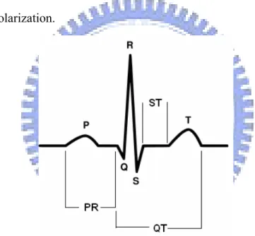
(17) beat begins with a signal from SA node. This is why the SA node is sometimes called “natural pacemaker of the heart”. The electrical impulses (action potentials) spread across the cells of the right and left atria that cause the atria to contract. When the signal arrives at the AV node near the ventricles, it slows for an instant. The signal is released and moves to the Bundle of His. From the Bundle of His, the propagating route of electrical impulses is divided into left and right bundle branches through the Purkinje fibers that connect directly to the cells in the walls of the left and right ventricles. After the signal passes, the ventricular walls relax and await the signal of next cardiac cycle. In summary, the electrical-propagation pathway of a cardiac cycle is: SA node → atria → AV node → Bundle of His → Purkinje fibers → ventricles.. Fig. 2.1 Cardiac conduction system.. A typical ECG tracing of a normal heartbeat (or cardiac cycle) consists of a P wave, a QRS complex and a T wave, as shown in Fig. 2.2. The physiological meaning. 6.

(18) of each ECG component is described below: P wave: During atrial depolarization, electrical impulses initiated by SA node propagate towards the AV node, and spread from the right atrium to the left atrium. This turns into the P wave on the ECG. QRS complex: this component represents ventricular depolarization. Activation of the anterioseptal region of the ventricular myocardium corresponds to the negative Q wave. The R wave is the point when half of the ventricular myocardium has been depolarized. T wave: The T wave represents ventricular repolarization and is longer in duration than depolarization.. Fig. 2.2 Typical wave complex of ECG.. PR interval: The PR interval corresponds to the time between the end of atrial depolarization to the onset of ventricular depolarization. ST interval: The ST interval represents the period from the end of ventricular depolarization to the beginning of ventricular repolarization. QT interval: The QT interval begins at the onset of the QRS complex and to the end of the T wave. It represents the time between the start of ventricular 7.

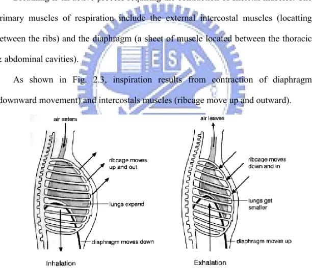
(19) depolarization and the end of ventricular repolarization. It is useful as a measure of the duration of repolarization.. 2.1.2 Introduction to Respiratory Signals Primary function of respiration is to supply oxygen to the body cells and eliminate carbon dioxide produced by cells. During inhalation, pathway of air is: nasal cavities (or oral cavity) > pharynx > trachea > primary bronchi (right & left) > secondary bronchi > tertiary bronchi > bronchioles > alveoli (site of gas exchange). Breathing is an active process requiring the contraction of skeletal muscles. The primary muscles of respiration include the external intercostal muscles (locatting between the ribs) and the diaphragm (a sheet of muscle located between the thoracic & abdominal cavities). As shown in Fig. 2.3, inspiration results from contraction of diaphragm (downward movement) and intercostals muscles (ribcage move up and outward).. Fig. 2.3 Mechanics of inhalation (inspiration) and exhalation (expiration). Inspiration mechanism: Contraction of external intercostal muscles > elevation of ribs & sternum > 8.

(20) increased front- to-back dimension of thoracic cavity > lowers air pressure in lungs > air flows into lungs. Contraction of diaphragm > diaphragm moves downward > increases vertical dimension of thoracic cavity > lowers air pressure in lungs > air flows into lungs. Expiration mechanism: Relaxation of external intercostal muscles & diaphragm > return of diaphragm, ribs, & sternum to resting position > restores thoracic cavity to preinspiratory volume > increases pressure in lungs > air is expired.. Respiration rate is the number of breaths in one-minute duration. The rate is usually measured when a person is at rest and simply involves counting the number of breaths for one minute.. 2.2 Wavelet Transformation. Time-frequency signal analysis offers a comprehensive and inspired knowledge for better interpreting data both in time and frequency. It allows researchers to observe those local, transient or intermittent components. Several time-frequency methods are available for signal analysis, for examples, short-time Fourier transform (STFT), Wigner–Ville transform (WVT), Choi–Williams distribution (CWD), and wavelet transform (WT). The continuous wavelet transform (CWT) is one of the favorite tools used by researchers since wavelet transform has been developed for many applications in recent years. Wavelet transform enables time-frequency representations of the signal, with versatile resolutions: high resolution in time and low resolution in frequency for 9.

(21) high-frequency components, whereas low resolution in time and high in frequency for low-frequency components [14]. Wavelet transform can be implemented by either CWT or DWT (discrete wavelet transform) computational algorithms. In this work we applied the CWT-based algorithm for better manipulation of the time-frequency coefficients. Let C(a,b) denote the wavelet transform of a continuous time signal, x(t), relative to basic wavelet Ψ(t) at scale a and window-center time b. Wavelet transform is defined as the inner product between the complex-conjugate function Ψ*(t) and the signal function x(t): +∞. C (a, b) = x(t ),ψ a ,b (t ) = ∫−∞ x(t )ψ a∗,b (t )dt. (2.1). where Ψ(t) is called the “mother wavelet” and its complex conjugate Ψ*a,b(t) is defined as: ⎛t −b⎞ (2.2) ⎟ a ⎝ a ⎠ In this study we used the Morlet wavelet as mother wavelet [14] (the real valued. ψ a∗,b (t ) =. 1. ψ⎜. Morlet wavelet is selected for CWT in order to isolate peaks and to distinguish positive and negative changes in the waveform) which is defined as follows,. ψ (t ) = cos(ω 0 t )e. 2 ⎞ − ⎛⎜ t ⎟ ⎝ 2⎠. (2.3). where ωo is the central frequency of the mother wavelet. Previous investigators have concentrated on wavelet transforms with ωo in the range 5–6 rad/s, where it can be performed without the correction term since it becomes very small. Fig. 2.4 below is the model of the real part of Morlet mother wavelet.. 10.

(22) Fig. 2.4 Morlet mother wavelet (real part).. The term of scale in wavelet sometimes can be treated as frequency. The pseudo-frequency is a term which describes the relationship between scale and frequency, and it presents a broad sense of frequencies that exist in a signal. To obtain pseudo-frequency we have to calculate the central frequency Fc of the wavelet and use the following relationship:. Fa =. Fc a⋅Δ. (2.4). where a is a scale, Δ is the sampling period, Fc is the center frequency of a wavelet (Hz), Fa is the pseudo - frequency corresponding to the scale a (Hz).. The contribution to the signal energy E(a,b) at the specific a scale and b location is given by the two-dimensional wavelet energy density function known as the scalogram (analogous to the spectrogram—the energy density surface of the STFT). The scalogram is defined below:. 11.

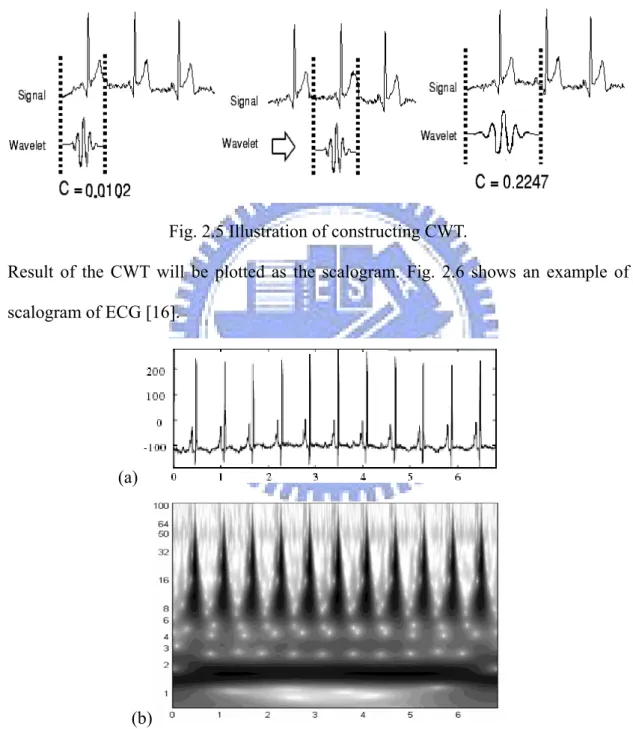
(23) E ( a, b) = C ( a, b) 2. (2.5). The schematic illustration for performing CWT is demonstrated in Fig. 2.5 that shows the scaling and shifting of mother wavelet [15].. Fig. 2.5 Illustration of constructing CWT. Result of the CWT will be plotted as the scalogram. Fig. 2.6 shows an example of scalogram of ECG [16].. (a). (b) Fig. 2.6 (a) Original ECG signal, (b) Morlet based scalogram of (a).. 12.

(24) 2.3 Quantification of Wavelet Coefficients Each ECG complexes create particular patterns in the wavelet scalogram. This study aimed to find degree of matching between these ECG wavelet patterns by quantifying the wavelet coefficient patterns. We proposed four methods that will be described in the next four sub-sections.. 2.3.1 Hu’s Invariant Moments Moment Invariants are mostly used for pattern recognition and shape descriptor. There are two types of shape descriptors: contour-based and region-based shape descriptor. Regular and widely used shape descriptor was derived by Hu [17]. This method has been used to recognize visual patterns or images that are independent of position, scale and orientation [18]. Geometric moment invariant introduced by Hu is derived from the theory of algebraic invariant. Two-dimensional moments of an M × M image with function of f(x, y), 0≤ x,y≤ M−1 are defined as: M −1 M −1. m pq = ∑ ∑ ( x) p .( y ) q f ( x, y ) x =0 y =0. (2.6). where p, q (order of moment) = 0, 1, 2, 3 ... Then the central moments can be defined as. μ pq = ∑∑ ( x − x ) p .( y − y ) q f ( x, y ) x. (2.7). y. where. x=. m10 m and y = 01 m00 m00. When a scaling normalization is applied, the normalized central moments ηpq are,. 13.

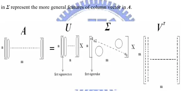
(25) η pq =. μ pq p+q ,γ = +1 γ 2 μ 00. (2.8). Hu defined seven invariant moments, computed by normalizing central moments through order of three. These seven moments are invariant to scale, position and orientation. The seven invariant moments are given below:. φ1 = η 20 + η02. (2.9.1). φ2 = (η 20 − η02 ) + 4η112 2. (2.9.2). φ3 = (η30 − 3η12 ) + ( 3η 21 − η03 ). 2. (2.9.3). φ4 = (η30 + η12 ) + (η 21 + η03 ). 2. (2.9.4). 2. 2. 2 2 φ5 = (η30 − 3η12 )(η30 + η12 ) ⎡(η30 + η12 ) − 3 (η21 + η03 ) ⎤ +. ⎣. ⎦. 2 2 ( 3η21 − η03 )(η21 + η03 ) ⎡⎣3 (η30 + η12 ) − (η21 + η03 ) ⎤⎦. (2.9.5). 2 2 φ6 = (η20 − η02 ) ⎡(η30 + η12 ) − (η21 + η03 ) ⎤ + 4η11 (η30 + η12 )(η21 + η03 ) (2.9.6). ⎣. ⎦. 2 2 φ7 = ( 3η 21 − η03 )(η30 + η12 ) ⎡(η30 + η12 ) − 3 (η21 + η03 ) ⎤ +. ⎣. ⎦. ( 3η12 − η30 )(η21 + η03 ) ⎡⎣3 (η30 + η12 ) − (η21 + η03 ) ⎤⎦ 2. 2. (2.9.7). 2.3.2 Singular Value Decomposition (SVD) Singular value decomposition (SVD) is one important algorithm developed on the basis of matrix algebra. SVD has been applied to several areas, including fetal ECG extraction [19], image processing [20], filter design [21], data compression theory [22], etc. In this study, SVD integrated with correlation-coefficient analysis was adopted to quantify the distribution property of wavelet coefficients. Consider a matrix A with dimension n×m, there exists a n×n unitary matrix U (orthogonal if A is real), an m x m unitary matrix V (orthogonal if A is real) and an n x m matrix Σ = diagonal (σ1, …σs) ≥ 0 with σ1≥ σ2≥…≥ σs≥ 0, where s=min{n, m}, such. 14.

(26) that the singular value decomposition A = UΣ V T. (2.10). The elements σs are called the singular values (eigenvalues) of A and are non-negative numbers. The matrix U contains the left singular vectors of B (eigenvectors of A), and the matrix V contains the right singular vectors (weighting vectors for reconstructing matrix A), as illustrated in Fig. 2.7. The eigenvalues in matrix Σ represent the ‘energy’ distribution of data in matrix A, while each eigenvector in matrix U is involved with the characteristics of the column vectors in matrix A. The eigenvectors corresponding to the larger eigenvalues in Σ represent the more general features of column vector in A.. Fig. 2.7 Singular Value Decomposition.. 2.3.3 Correlation Coefficient Evaluation of correlation coefficient (γ) provides a way to statistically measure strength and direction of a linear relationship between two signals, vectors, images or just random variables. Two-dimensional cross-correlation analysis is a method frequently used for pattern recognition in digital image processing [23]. Two-dimensional. cross. correlation. was. also. evaluated. between. template. spectra-temporal maps to detect beat-to-beat late potential activity [24]. But in this 15.

(27) work, one-dimensional correlation coefficients were computed to evaluate ECG wavelet pattern. Defined Pearson’s one-dimensional correlation coefficient (γ) below,. γ ( x, y ) =. n∑ xy − ∑ x ∑ y 1 2. {(n∑ x − (∑ x ))(n∑ y − (∑ y ))} 2. 2. 2. 2. (2.12). where X and Y are two vectors to be compared. The value of γ is in the range -1 < γ < +1. The + and – signs indicate positive U. U. U. U. linear correlations and negative linear correlations, described briefly below: •. Positive correlation: if x and y have a strong positive linear correlation, γ is close to +1. A γ value of exactly +1 indicates a perfect positive match. In the case of positive correlation, values of y increase as values of x increase.. •. Negative correlation: if x and y have a strong negative linear correlation, γ is close to -1. A γ value of exactly −1 indicates a perfect negative match. In the case of negative correlation, values of y decrease as values of x increase.. •. No correlation: if there is no linear correlation or a weak linear correlation, γ is close to 0. A value near zero means that there exists the random, nonlinear relationship between two variables. 2.3.4 Analysis of Variance (ANOVA) ANOVA is a statistical tool to show whether data from several groups could be accounted for by the hypothesized factor. The objective of single-factor ANOVA problem is to decide whether the means for more than two treatments are identical [25]. In [26], ANOVA was used to compare stego-images (images that have been manipulated by steganographic methods) of several groups. There are two types of ANOVA: one-way and two-way ANOVA. One-way 16.

(28) ANOVA was employed in this study. The assumption of ANOVA is that test data are normally distributed. Table 2.1 typical data for one-way ANOVA. Table 2.1 One-way ANOVA typical data Treatment. Observations. Totals. Averages. y1 .. 2. y21. y22…. .... y2n. y2 .. y2 .. .... a. ya1. ya2. .... …. y1 .. …. y1n. …. .... …. y12. …. y11. …. 1. yan. ya .. ya .. y... y... Let yi. represents the total of the observations under the ith treatment and y i . represents the average of the observations under the ith treatment. Similarly y.. represents the grand total of all observations and y.. represents the grand mean of all observations. Procedure of analyzing one-way ANOVA is described below. 1. Set null hypothesis H0 and alternative hypothesis H1 for the comparison of independent groups. H0: τ1 = τ2 =… τα = 0; Means of all the groups are equal. H1: τi ≠ 0 for at least one i; Means of two or more groups are not equal.. 2. Compute Sum of Squares Deviations of treatment, Error Sum of Squares and each freedom degrees.. 17.

(29) Sum of Squares Deviations of treatment: 2. a. SSTr = n ∑ ( y i . − y..) i =1. (2.13). Error Sum of Squares: SSE = ∑ ∑ ( y ij − y i .) a. 2. n. i =1 j =1. (2.14). Freedom degrees of SSTr and SSE are dftr = a-1 and dfe = a(n-1). 3. Compute Mean Square for treatment and Mean Square of error Mean square for treatment MSTr: MSTr =. SSTr df tr. (2.15). SSE df e. (2.16). Mean square of error MSE: MSE =. 4. Compute the F-test: Fa =. MSTr MSE. (2.17). 5. Determine the significant level and select test statistics For given a significant level a (in this study 0.05), the cumulative probability of F > Fa is P{ F > Fa}, then P value = 2 * P{ F > Fa}. If F > Fa then we accept null hypothesis that the means of the groups are equal, otherwise we reject null hypothesis that means the groups are not equal. Also we give a significant level of 0.05, so any results of P value under 0.05 will be significant different (means of groups are not equal).. 18.

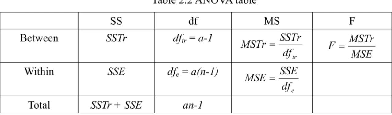
(30) In summary as in Table 2.2 below Table 2.2 ANOVA table SS. df. Between. SSTr. dftr = a-1. Within. SSE. dfe = a(n-1). Total. SSTr + SSE. an-1. MS SSTr MSTr = df tr MSE =. F F=. MSTr MSE. SSE df e. Couderc et al. [11] used wavelet coefficient and ANOVA method to quantify ECG abnormalities of patients with and without ventricular tachycardia and long QT syndrome. The result of their work brings a new way of the ECG signal analysis. The same algorithm was used by N. Selmaoui [27] for detecting risks of sudden cardiac death on the patients who survived from acute myocardial infarction.. 19.

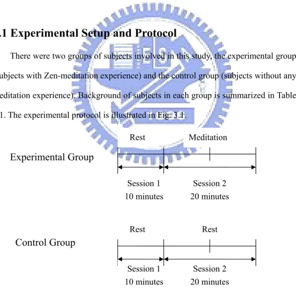
(31) Chapter 3 Experiment and Signal Analysis We will first introduce the experimental setup and protocol used in this study. In the second part, the implementation strategies and parameters are presented, including the procedure of applying wavelet transform to the raw ECG signal and quantifying the wavelet coefficient data.. 3.1 Experimental Setup and Protocol There were two groups of subjects involved in this study, the experimental group (subjects with Zen-meditation experience) and the control group (subjects without any meditation experience). Background of subjects in each group is summarized in Table 3.1. The experimental protocol is illustrated in Fig. 3.1. Rest. Meditation. Experimental Group Session 1 10 minutes. Rest. Session 2 20 minutes. Rest. Control Group Session 1 10 minutes Fig. 3.1 Experimental protocol.. 20. Session 2 20 minutes.

(32) Table 3.1 Subjects of experimental and control groups Experimental group. Control group. Number of subjects. 8. 9. Gender (male : female). 5:3. 8:1. Age (years). 26.1 ± 2.1. 25.3 ± 3.3. Meditation experience (years). 5 ± 3.4. The experiments included two continuous sessions (sessions 1 and 2). During Session 1, subjects of both groups rested with eyes closed for 10 minutes. During Session 2, subjects of control group continued resting for 20 minutes. On the other hand, experimental subjects began meditation for 20 minutes. The Experimental subjects meditated with either full-lotus or half-lotus posture, with eyes closed. All subjects breathed naturally in both sessions. ECG and respiratory signals were measured using PowerLab biosignal recording system (ADInstruments, Sydney, Australia) and then displayed and saved on a personal computer using the software Chart4 (ADInstruments, Bella Vista, Australia), as shown in Fig. 3.2.. 3.1.1 Measurement of ECG Signal The ECG signal was recorded using Lead I of standard bipolar limb leads (frontal plane), as shown in Fig. 3.3(a). Electrode site on the left (right) arm was connected to the amplifier’s positive (negative) input, with the ground on the inside of left ankle. The disposable ECG electrodes (Medi-Trace 200 Foam Electrodes, Kendall, USA) as shown in Fig. 3.3 (b) were used on the experiment. The ECG was pre-filtered by a 0.3-200 Hz bandpass filter and digitized by a sampling rate of 1000 Hz.. 21.

(33) Physiological signal. Physiological signal recording system (PowerLab). USB port. Personal Computer (Chart4 software). Fig. 3.2 The physiological signal recording system.. (a). (b). Fig. 3.3 (a) LeadⅠconfiguration of bipolar limb leads, (b) Disposable ECG electrode.. 3.1.2 Measurement of Respiratory Signal Respiratory signals were recorded using piezo-electric transducer as shown in Fig. 3.4 (model 1132 Pneumotrace II (R), UFI, Morro Bay, CA, USA). The transducer 22.

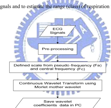
(34) was wrapped around the belly passing the navel. The respiration signal was pre-filtered by a lowpass filter with cutoff frequency 5 Hz and digitized at the sampling rate of 1000 Hz. An example of respiratory signal is shown in Fig. 3.5. The amplitude of respiration signal increases during inspiration and decreases during expiration.. Fig. 3.4. Piezo-electric respiratory transducer.. Inspiration Expiration. 3. Amplitude. 2 1 0 -1 -2. 0. 2. 4. 6. 8. 10. 12. 14. 16. 18. 20. Time (second) Fig. 3.5 Respiratory signal.. 3.2 Wavelet Transform of ECG Signal We performed the continuous wavelet transformation on raw ECG signals. The flow chart of wavelet transform is shown in Fig. 3.6. The first step is the pre-processing stage where the R peaks of ECG and the inspiration peaks were detected. In addition, respiration rate was estimated; and band-pass filter was applied 23.

(35) to ECG to remove baseline drift and other noises. For the pre-processed ECG signal, the scale (frequency) parameter was determined to perform continuous wavelet transform. Finally, CWT coefficients of interest were stored for further, advanced analysis.. Step 1. Pre-processing We focused on the frequency range of 2-40 Hz for ECG signals [28] to preserve P, QRS, and T components of ECG. In this pre-processing stage, both the ECG and respiratory signals were down-sampled to the rate of 200 samples per second. Then algorithm in Appendix A was applied to detect R peaks of ECG and inspiration peaks of respiratory signals and to estimate the range (class) of respiration rate.. Fig. 3.6 Flow chart of continuous wavelet transforms.. Step 2. Determination of CWT parameters To perform continuous wavelet transformation, we need to define the parameters such as scale, mother wavelet, etc.. 24.

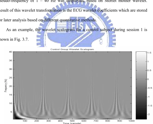
(36) The scale a can be determined by equation (2.4) as follows: scale =. Fc , Fa ⋅ Δ. where Δ is the sampling period, Fc is the center frequency of a wavelet (Hz), Fa is the pseudo - frequency corresponding to the scale (Hz). In our study, Morlet prototype was adopted as mother wavelet, where ω0 = 5 rad/s.. Step 3. CWT analysis and evaluation To perform CWT computation, the MATLAB build-in function with a pseudo-frequency of 1 – 40 Hz was employed, based on Morlet mother wavelet. Result of this wavelet transformation is the ECG wavelet coefficients which are stored for later analysis based on different quantitative methods. As an example, the wavelet scalogram for a control subject during session 1 is shown in Fig. 3.7.. Fig. 3.7 The wavelet scalogram of a control subject during Session 1.. 25.

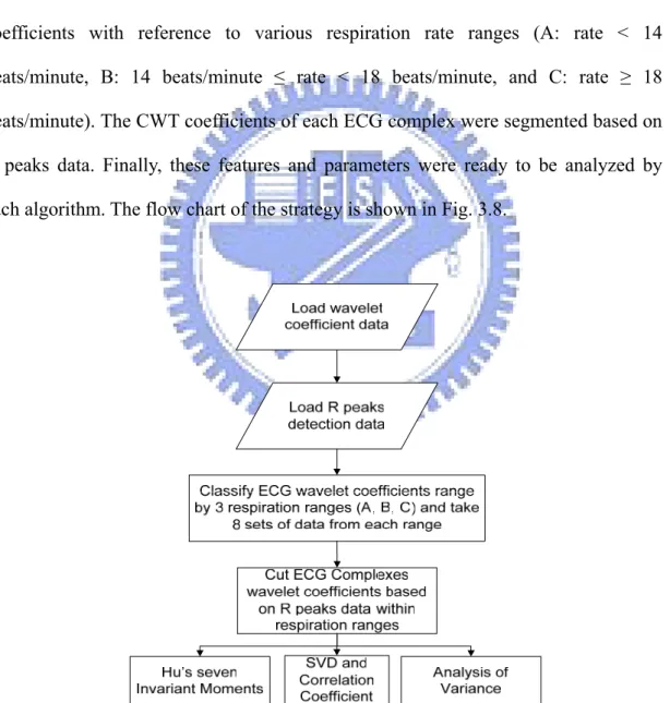
(37) 3.3 Quantification of Wavelet Coefficients In this section, we will describe the strategies for quantifying the wavelet-coefficient patterns produced by continuous wavelet transform. Three different methods having been introduced in chapter 2 were applied: Hu’s invariant moments, SVD with correlation coefficient, and the ANOVA analysis. The analysis of each method requires the following features derived at the first stage, that is, the R peaks detected and CWT coefficients. We analyzed CWT coefficients with reference to various respiration rate ranges (A: rate < 14 beats/minute, B: 14 beats/minute ≤ rate < 18 beats/minute, and C: rate ≥ 18 beats/minute). The CWT coefficients of each ECG complex were segmented based on R peaks data. Finally, these features and parameters were ready to be analyzed by each algorithm. The flow chart of the strategy is shown in Fig. 3.8.. Fig. 3.8 Flowchart of CWT quantification strategy.. 26.

(38) Fig. 3.9 illustrates the results of extracted R-based ECG complexes, corresponding wavelet coefficients, and the respiration rate (range-A, -B, or -C). In Fig. 3.9 (a), the R peaks detected are marked with ‘*’. The window size we used is 46 time points left side and 75 time points right side from R peaks, so total size is 122 time points wide. Based on these R peaks, we extracted ECG wavelet-coefficient array within the same, constant frame. The resulted wavelet ‘image’ is shown in Fig. 3.9 (b).. (a) Fig. 3.9 (a) Extraction of ECG complexes based on R peaks (b) One ECG complex wavelet coefficient template.. 27.

(39) (b) Fig. 3.9 (Continued). In Fig. 3.9 (b), the dark curve is one ECG complex in alignment with the distribution of wavelet coefficients.. 3.3.1 Invariant Moments Analysis The implementation of Hu’s invariant moments algorithm in our study directly followed equations (2.6)-(2.9), as shown in Fig. 3.10.. Fig. 3.10 Flow chart of Hu’s Invariant Moments Algorithm. 28.

(40) Here, the CWT coefficients were displayed in logarithmic scale to reduce dynamic range. In addition, moment-invariant analysis was applied to absolute CWT coefficients to avoid dealing with the complex number.. (b) Φ1. Φ2. Φ3. Φ4. Φ5. Φ6. Φ7. Mean. 4.39. 5.88. 11.24. 11.21. 22.42. 14.48. 19.48. std. 0.93. 2.29. 3.15. 3.17. 6.33. 4.27. 5.63. Fig. 3.11 (a) Wavelet coefficient of one subject from control group, (b) Seven invariant moments values.. Fig. 3.11 (b) demonstrates the results of analyzing Hu’s invariant moments of CWT coefficients for one control subject.. 3.3.2 SVD Integrated with Correlation Coefficient The second scheme we proposed to quantify wavelet coefficients was singular value decomposition integrated with correlation-coefficient analysis. ECG CWT coefficients were treated as a two dimensional matrix that was further decomposed with SVD into U, Σ and V. The flow chart of this algorithm is shown in Fig. 3.12.. 29.

(41) Fig. 3.12 Flow chart of SVD and correlation coefficient algorithm.. Fig. 3.13 displays an example to illustrate the whole process of SVD and correlation-coefficient analysis scheme. First we averaged 8 sets data of ECG-complex CWT-coefficient matrices from each respiration rate range either on session 1 or session two. Then SVD analysis was performed on these average CWT-coefficient matrices from different respiration rates range. As a consequence, several matrices U were extracted from two different sessions of average CWT-coefficient matrices. As being well known, columns of matrix U contain eigenvectors corresponding to eigenvalues in diagonal matrix Σ. We took only the biggest eigenvalue (σ1) and the corresponding eigenvector in the first column of matrix U.. 30.

(42) Singular Value Decomposition. Average. Correlation Coefficient resulted γ. Average. Singular Value Decomposition. Fig. 3.13 Illustration of SVD Extraction algorithm. In Fig. 3.13 an illustration of SVD from control subject on slow respiration at both session. After we got the 1st eigenvectors from different respiration ranges, we then calculated the correlation coefficient γ between them.. 31.

(43) 3.3.3 Analysis of Variance (ANOVA) Procedure The illustration of ANOVA algorithm is shown in Fig. 3.14.. Fig. 3.14 Illustration of ANOVA algorithm.. The first step of ANOVA is to select wavelet coefficients at the same scale (frequency) a and time (sample) b position from several ECG-complex CWT-coefficient templates of two different sessions. Secondly, their p-value was evaluated through calculating their sum of square, mean square, and F-test as described in equations (2.13) – (2.17). The above scheme was conducted for all (scale, time) range of the ECG CWT-coefficient templates. For example, considering a CWT-coefficient template of size 79×122, then there required totally 79×122 repetitions.. 32.

(44) Fig. 3.15 demonstrates the flowchart of conducting ANOVA in our study.. Fig. 3.15 Flowchart of ANOVA algorithm.. The result of this ANOVA algorithm is the map of p-values that measure how significant the difference between two populations. To demonstrate the result, we mapped the p-values onto the same time-frequency plane as the CWT-coefficient template. We defined significantly different into two types (increasing or decreasing energy) based on wavelet energy (eq. 2.5) comparison. For example we got one of the P-value = 0.02 (considered as significantly different) from the ANOVA between slow breathing and fast breathing on session 1 of control group, then we have to test the wavelet energy between these comparison: if slow breathing > fast breathing we called increasing energy, other than that decreasing energy. So increased energy are given as positive p-value colored red and depressed energies are given as negative p-value colored blue. Void-colored pixel indicates the condition of being NOT significant so called NOT Significant colored white. These p-values are ranked according to color scale.. 33.

(45) Fig. 3.16 P-value Map as result of ANOVA.. 34.

(46) Chapter 4 Results This chapter presents the results of applying invariant moments, SVD and ANOVA to quantification of ECG-complex CWT-coefficient behaviors in various respiration-rate ranges.. 4.1 Results of Invariant Moments Analysis In this section, we will present the results of invariant moments analysis applied to ECG wavelet coefficients. Hu’s invariant moments are normally adopted for pattern recognition. This study, however, was aimed to use the invariant moments to quantify the differences of ECG CWT coefficients in different conditions. We compared seven invariant moments derived from three respiration-rate ranges. The results are summarized in Table 4.1 and further explained in the following sub-section.. Table 4.1 Mean values of three respiration rate ranges analyzed for the experimental and control group on session 1 and 2. Seven Invariant Moments of Control Group Session 1 Φ1. Φ2. Φ3. Φ4. Φ5. Φ6. Φ7. A. 5.7±0.3. 9.4±0.8. 15.2±0.9 15.1±0.9 30.3±1.9 20.1±1.3 25.9±2.1. B. 5.3±0.6. 8.5±1.7. 14.0±1.6 14.0±1.6 27.9±3.2 18.5±2.4 22.6±2.9. C. 4.8±0.6. 7.1±1.6. 12.7±1.9 12.6±1.9 25.3±3.9 16.5±2.7 20.3±2.9. Seven Invariant Moments of Control Group Session 2 Φ1. Φ2. Φ3. Φ4. A. 5.0±0.2. 7.6±0.6. 12.9±0.6 12.7±0.6 25.5±1.3 16.8±0.8 22.1±1.6. B. 5.0±0.5. 7.7±1.4. 13.2±1.5 13.1±1.5 26.3±3.0 17.2±2.2 21.4±2.5. C. 4.8±0.6. 7.1±1.6. 12.5±1.9 12.5±1.9 25.1±3.8 16.4±2.7 19.8±3.4 35. Φ5. Φ6. Φ7.

(47) Seven Invariant Moments of Experimental Group Session 1 Φ1. Φ2. Φ3. Φ4. Φ5. Φ6. Φ7. A. 6.4±0.8 11.1±1.8 17.9±2.1 17.9±2.1 35.8±4.2. 23.6±3.0 30.2±4.1. B. 6.1±0.9 10.3±2.2 16.7±3.3 16.6±3.5 33.2±6.9. 21.8±4.7 28.0±5.5. C. 6.1±1.4 10.4±3.2 16.5±5.4 16.4±5.6 32.8±11.1 21.7±7.2 27.4±9.4 Seven Invariant Moments of Experimental Group Session 2 Φ1. Φ2. Φ3. Φ4. Φ5. Φ6. Φ7. A. 6.7±0.9 11.8±2.1 18.7±3.2 18.7±3.2 37.4±6.4. 24.8±4.2 31.5±5.4. B. 6.9±1.7 12.1±3.9 19.4±5.7 19.4±5.7 38.8±11.4 25.6±7.5 32.8±10.3. C. 8.1±2.2 14.8±4.8 23.3±7.4 23.3±7.4 46.6±14.8 30.9±9.8 39.3±13.8. 4.1.1 Comparison of Invariant Moments at Different Respiration Rates First comparison is conducted for results of analyzing ECG within the same session (session 1 or 2) yet in different respiration-rate ranges (A, B, C). Figs. 4.1 and 4.2 display the results of seven invariant moments for both control group and experimental group.. Phi Value. Invariant Mom ents Cont. Group S1 35 30 25 20 15 10 5 0. Φ1 Φ2 Φ3 Φ4 Φ5 Φ6 A. B. C. Respiration Rate Class. (a) Fig. 4.1 Result of Control Group Invariant Moments S1 and S2.. 36. Φ7.

(48) Phi Value. Invariant Mom ents Cont. Group S2 35 30 25 20 15 10 5 0. Φ1 Φ2 Φ3 Φ4 Φ5 Φ6 A. B. C. Φ7. Respiration Rate Class. (b) Fig. 4.1 (Continued).. Invariant Moments Expt. Group S1. Phi Value. 50. Φ1. 40. Φ2. 30. Φ3 Φ4. 20. Φ5. 10. Φ6 Φ7. 0 A. B. C. Respiration Rate Class. (a) Invariant Moments Expt. Group S2. Phi Value. 50. Φ1. 40. Φ2. 30. Φ3 Φ4. 20. Φ5. 10. Φ6 Φ7. 0 A. B. C. Respiration Rate Class. (b) Fig. 4.2 Result of Experimental Group Invariant Moment S1 and S2.. Apparently, seven invariant moments decrease with respiration rate for the control subjects during session S1. On the other hand, seven invariant moments 37.

(49) increase with respiration rate for the experimental subjects under meditation (session S2).. 4.1.2 Comparison of Invariant Moments in Different Sessions Given the same respiration rate, the results of invariant moments for subjects in different sessions are shown in Figs. 4.3 and 4.4, respectively, for control group and experimental group. Invariant Moments Cont.Group S1 VS S2 Slow Breath. Phi Value. 35 30. Φ1. 25. Φ2 Φ3. 20. Φ4. 15. Φ5. 10. Φ6. 5. Φ7. 0 A S1. A S2 Respiration Rate Class. (a) Invariant Moments Cont.Group S1 VS S2 Normal Breath 30 Φ1. 25 Phi Value. Φ2 20. Φ3. 15. Φ4 Φ5. 10. Φ6 5. Φ7. 0 B S1. B S2 Respiration Rate Class. (b) Fig. 4.3 Seven invariant moments from S1 to S2 for respiration rate (a) A: slow breathing, (b) B: normal breathing, and (c) C: fast breathing (control group).. 38.

(50) Invariant Moments Cont.Group S1 VS S2 Fast Breath 30 Φ1. Phi Value. 25. Φ2. 20. Φ3. 15. Φ4 Φ5. 10. Φ6 5. Φ7. 0 C S1. C S2 Respiration Rate Class. (c) Fig. 4.3 (Continued).. Invariant Moments Expt.Group S1 VS S2 Slow Breath 40.0. Phi Value. 35.0. Φ1. 30.0. Φ2. 25.0. Φ3. 20.0. Φ4. 15.0. Φ5. 10.0. Φ6 Φ7. 5.0 0.0 A S1. A S2 Respiration Rate Class. (a) Fig. 4.4 Seven invariant moments from S1 to S2 for respiration rate (a) A: slow breathing, (b) B: normal breathing, and (c) C: fast breathing (experimental group).. 39.

(51) Inv ariant M oments Expt.Group S1 VS S2 Normal Breath 45.0 40.0 Φ1. 35.0. Φ2. Phi Value. 30.0. Φ3. 25.0. Φ4. 20.0. Φ5. 15.0. Φ6. 10.0. Φ7. 5.0 0.0 B S1. B S2 Respiration Rate Class. (b) Invariant M ome nts Expt.Group S1 VS S2 Fast Bre ath 50.0. Phi Value. 45.0 40.0. Φ1. 35.0. Φ2. 30.0. Φ3. 25.0. Φ4. 20.0. Φ5. 15.0. Φ6. 10.0. Φ7. 5.0 0.0 C S1. C S2 Respiration Rate Class. (c) Fig. 4.4 (Continued).. While comparing the invariant moments between sessions (Figs. 4.3 and 4.4), we notice that the seven invariant moments tend to decrease for control group, yet increase for experimental group when proceeding from session one to session two. In [17], Hu interpreted two physical meanings of seven invariant moments, that is, φ1 = μ 20 + μ 02 and. φ 2 = (μ 20 − μ 02 )2 + 4 μ112 respectively reflecting “spread”. and “slenderness”. These two invariant moments have been also employed in the 40.

(52) interpretation of the spread and slenderness of gene [29]. Fig. 4.5 sketches. φ2. versus φ1 curves for (a) control and (b) experimental group in sessions S1 (left) and S2 (right).. (a). (b) Fig. 4.5 Second order moments in (a) control group and (b) experimental group. 41.

(53) Apparently, the range of φ1 and. φ 2 changes from session S1 to session S2. for both groups. For control group, the second order moments seem to cluster together in S2, but spread out in S1. Whereas for experimental group, second order moments clustered in S1, yet spread in S2. At the current stage, we still cannot correlate our preliminary findings to the physiological meanings of circulatory system.. 4.2 Results of Singular Value Decomposition Analysis The goal of SVD analysis is to extract the major component of the ECG wavelet coefficients and try to identify the intra-session and inter-session differences by using the correlation-coefficient analysis. In Fig. 4.6, we present the results of analyzing two samples, one sample from control group and one sample from experimental group.. (a) Fig. 4.6 Singular value decomposition of (a) a control subject and (b) an experimental subject (from top: CWT-coefficient map, the first and the second eigenvector).. 42.

(54) (b) Fig. 4.6 (Continued).. Fig. 4.6 plots the two major components (1st eigenvector and 2nd eigenvector), decomposed by SVD, corresponding to the largest two eigenvalues. Their weighting percentages are listed in Table 4.2. The 1st eigenvalue contributes the biggest portion to the CWT-coefficient map. Table 4.2 Weighted percentage of each eigenvalues CONTROL. EXPERIMENTAL. GROUP. GROUP A (Slow Breath). eigenvector weighted percentage. 1st. 2nd. 19.3 %. 14.9 %. A (Slow Breath) eigenvector weighted percentage. 1st. 2nd. 18.4%. 13.9%. Later in our study, we only analyzed the 1st eigenvector. Comparisons and correlation-coefficient analysis will be conducted for both groups under various conditions: different respiration rates as well as different sessions S1 and S2.. 43.

(55) (a). (b) Fig. 4.7 (a) Control Subject and (b) Experimental subject 1st eigenvector and their correlation coefficient between respiration ranges. 44.

(56) Table 4.3 is the summary of correlation coefficient between various respiration rates and between recording sessions for control and experimental group.. Table 4.3 Correlation-coefficient analysis of the first eigenvector of ECG-complex CWT-coefficient maps. EXPERIMENTAL GROUP Correlation coefficient Session 1 B A. Correlation coefficient Session 2. C. 0.9976. B. B -0.99436. A. -0.99763. B. C 0.9953. 0.96552 0.98096. Correlation coefficient different sessions S2 A. C. 0.99472. A S1. B. 0.9966. B. -0.97052. C. CONTROL GROUP Correlation coefficient Session 1 B A. Correlation coefficient Session 2. C 0.99235. B. 0.91251. A. 0.94545. B. B. C. 0.86111. 0.95564 0.92572. Correlation coefficient different sessions S2 A A S1. B. C. 0.74461* 0.99953. B. 0.99631. C. A < 14 beats/minute; 14 beats/minute≤ B <18 beats/minute;, C≥18 beats/minute; S1 = session 1; S2 = session2; *correlation coefficient below 0.85 (moderate correlation).. 45.

(57) Fig. 4.8 Control subject 1st eigenvector between S1 and S2 slow breathing. As we can see from table 4.3 that most of correlation coefficient values is considered high (highly correlate), only one result considered moderate correlation. So we need to see the results came from ANOVA analysis in next subchapter.. 4.3 Results of ANOVA ANOVA analysis provides a way to evaluate the degree of statistical significance of quantitative results obtained by previous methods, under various experimental conditions.. 46.

(58) Fig. 4.9 ANOVA analysis for control group (intra-session, different rates of respiration).. 47.

(59) Fig. 4.10 analysis for experimental group (intra-session, different rates of respiration).. In the first part, ANOVA analysis was conducted for the quantitative results obtained in the same session, yet under different respiration rates. Figs. 4.8 and 4.9 plot respectively the ANOVA results for the control and experimental group. Different colors (red and blue) are used to indicate positive significantly increasing energy and negative significantly decreasing energy, while color-void indicates no significant 48.

(60) difference. We used the wavelet energy to make comparison between wavelet coefficient in term of The color degraded from dark blue or red (p-value < 0.01) to indicate more significant to light blue or red (p-value < 0.05) just plain significant. We observe that, during either session S1 or S2 in control group, significant difference occurred between slow breathing and fast breathing especially at S-T segment (decreasing energy since it colored blue). Moreover, results of analyzing QRS complex revealed significantly decreasing energy between slow breathing and normal breathing on session S2. Other condition had few significant differences as in S1 and S2 fast breathing compared with normal breathing, significantly decreasing energy on high frequency at S-T segment also occurred. If we see the ANOVA result on experimental group there were significant differences in S1; slow breathing compared with fast breathing, slow breathing compared with normal breathing, and session two slow breathing compared with normal breathing. In session one between slow and fast breathing occurred significantly increasing energy on S-T segment at the high frequency. It even had more significantly increasing energy between slow and normal breathing in session one. We can see there was significantly decreasing energy spread along P-QRS-T area at frequency between 5 – 20 Hz in session two between slow and normal breathing rate.. 49.

(61) Fig. 4.11 ANOVA analysis for Control Group (inter session, same rates of respiration) 50.

(62) Fig. 4.12 ANOVA analysis for Experimental Group (inter session, same rates of respiration) 51.

(63) Fig. 4.10 and Fig. 4.11 are results from applied ANOVA between sessions on both groups. We take three comparison based on three respiration ranges between S1 and S2. In control group we found both significantly little increasing and more decreasing energy (p-value <0.01) spread on ECG complex when we performed ANOVA to investigate slow breathing between both sessions, while on fast breathing we even didn’t find any significant difference and normal breathing we did not found big significant difference. In experimental group we found significantly increasing energy on slow breathing between S1 and S2. The contrary to slow breathing is on fast breathing between S1 and S2, we found significantly decreasing energy occurred in several ECG segment either low or high frequency. On normal breathing of experimental group between both sessions we just found small significant difference on T segment at frequency around 23 – 27 Hz.. 52.

(64) Chapter 5 Conclusion and Discussion 5.1 Preliminary Conclusion In this study we have studied the applications of continuous wavelet transformation to ECG analysis. The main aim of this thesis was to investigate the effects of Zen meditation on the ECG wavelet coefficients of the experimental (meditating) and control (non-meditating) group. In this study, respiration rate was adopted as a reference for comparing ECG time-frequency properties. In chapter 4, we have reported the results obtained by Hu’s invariant-moment analysis, correlation-coefficient analysis of SVD components, and ANOVA approach. In regard to the study of Hu’s invariant moment on ECG CWT-coefficient maps, on control group the values of seven invariant moments, at a given respiration rate, tended to decrease for the control group, while the values for the experimental group showed the tendency of increase. According to the second order moments, we may conclude that control group has wavelet coefficient patterns more concentrated than experimental group by the value of φ 2 =. (μ 20 − μ 02 )2 + 4μ112 . At the current stage,. we are, however, still not ready to correlate the physiological meaning with each particular invariant moment due to insufficient amount of data. In the SVD study, experimental group exhibited large correlation correlations in most of the comparisons, indicating that the major components of wavelet coefficients are close to each other. While in control group, we notified one moderate correlation-coefficient value on comparison between sessions S1 and S2 slow. 53.

(65) breathing state, but still most results had high correlation coefficient values. Finally, ANOVA analysis provides a way to evaluate the significance of differences of ECG CWT-coefficient templates. The results reported in chapter 4 revealed more significant differences in control group than in experimental group. In control group the tendency of significantly differences is decreasing energy in some segments of ECG wavelet coefficients, as in slow breathing compared with fast breathing on both sessions S1 and S2. On the other hand, the tendency of significance in experimental group appeared to be the increasing energy as in slow breathing compared with fast or normal breathing on S1.. 5.2 Future Work In the preliminary study, we presented the idea and results of applying Hu’s seven invariant moments. Further study is to be conducted to correlate the quantitative results with the physiological meaning. In addition, other image-based methods or approaches can be investigated and employed in the analysis of ECG (or other physiological signals) CWT-coefficient templates. Finally, experimental protocol may be designed to include EEG signals as the reference, in addition to the respiration signal, of various consciousness, mental, or even meditation states.. 54.

(66) References [1] Chitrapu P. R., Waldo D. J., “Time-frequency analysis and linear prediction of cardiac late potentials,” Proceedings of the IEEE-SP International Symposium, pp. 227-230, 1992. [2] Millet-Roig J., Rieta-Ibanez J. J., Vilanova E., Mocholi A., Chorro F. J., “Time-frequency analysis of a single ECG: to discriminate between ventricular tachycardia and ventricular fibrillation,” Computers in Cardiology 1999, pp. 711-714, 1999. [3] Spaargaren A. and English M. J., “Analysis of the signal averaged ECG in the time-frequency domain,” Computers in Cardiology 1999, pp. 571-574, 1999. [4] Crowe J. A., Gibson N. M., Woolfson M. S., Somekh M. G.., “Wavelet transform as a potential tool for ECG analysis and compression,” J. Biomed. Eng., vol.14(3), pp. 268-272, 1992. [5] Provaznik I. and Kozumplik J., “Wavelet Transform in Electrocardiography - Data Compression,” International Journal of Medical Informatics, vol.45, pp.111-128, 1997. [6] Hilton M. L., “Wavelet and wavelet packet compression of electrocardiograms,” IEEE Trans. Biomed. Eng., vol.44(5), pp.394-402, 1997. [7] Li C., Zheng C., Tai C., “Detection of ECG characteristic points using the wavelet transform,” IEEE Trans. Biomed. Eng., vol.42, pp.21-28, 1995. [8] Bahoura M., Hassani M., Hubin M., “DSP implementation of wavelet transform for real time ECG wave forms detection and heart rate analysis,” Comp. Methods & Programs Biomedicine, vol.52, pp.35-44, 1997.. 55.

(67) [9] Wiklund U., Akay M., Niklasson U., “Short-term analysis of heart-rate variability by adapted wavelet transforms,” IEEE Eng. Med. Biol., vol.16 pp.113-138, 1997. [10] Carvalho J. L. A., Rocha A. F., Junqueira Jr. L. F., Souza Neto J., Santos I., Nascimento F.A.O., “A Tool for Time-Frequency Analysis of Heart Rate Variability,” Proceedings of the 25th Annual International Conference of the IEEE EMBS, pp. 2574-2577, 2003. [11] Couderc J. P., Fareh S., Chevalier Ph., et al., “Stratification of time-frequency abnormalities in the signal-averaged high-resolution ECG in postinfarction patients with and without ventricular tachycardia and congenital long QT syndrome,” J. Electrocardiol. 1996, vol.29, pp.180–188, 1996. [12] Couderc J. P., Chevalier P., Fayn J., Rubel P., Touboul P., “Identification of post-myocardial infarction patients prone to ventricular tachycardia using time–frequency analysis of QRS and ST segments,” Europace 2000, vol.2(2), pp.141-153, 2000. [13] Peng C.K. , Mietus J. E., Liu Y., Khalsa G., Douglas P. S., Benson H., Goldberger A.L., “Exaggerated heart rate oscillations during two meditation techniques,” International Journal of Cardiology, vol.70(2), pp.101－107, 1999. [14] Ilic S., “Detection of the left bundle branch block in continuous wavelet transform of ECG signal,” Electronics and Electrical Engineering, vol. 2(74), pp. 33–36, 2007. [15] Michel M.,Yves M., et al., “Wavelet Toolbox 4 User’s Guide,” The MathWorks Inc., Massachusetts, 2007. [16] Addison P. S., “Wavelet transforms and the ECG: a review, ” Physiological Measurement, vol.26(5), pp. R155-R199, 2005. [17] Hu M. K., “Visual pattern recognition by moment invariants,” IRE Trans. Information Theory, vol.8, pp. 179–187, 1962. 56.

(68) [18] Noh J. S., Rhee K. H., “Palm print Identification Algorithm Using Hu Invariant Momentsand Otsu Binarization,” Proc. of the 2nd FSKD, LNAI 3614, pp.91-94, 2005. [19] Al Zaben A., Al Smadi A., “Extraction of foetal ECG by combination of singular value decomposition and neuro fuzzy inference system,” Physics in medicine and biology, vol. 51(1), pp. 137-143, 2006. [20] H.C. Andrews and C.L. Patterson, “Singular Value Decompositions and Digital ImageProcessing,” IEEE Trans. ASSP, pp. 26-53, 1976. [21] T.-B. Deng and M. Kawamata, “Frequency-domain design of 2-D digital filters using the iterative singular value decomposition,” IEEE Transactions on Circuits and Systems, vol. 38, no. 10, pp. 1225-1228, 1991. [22] J.-J. Wei, C.-J. Chang, N.-K. Chou, and G.-J. Jan, “ECG data compression using truncated singular value decomposition,” IEEE Transactions on Information Technology in Biomedicine, vol. 5, no. 4, pp. 290-299, 2001. [23] Gonzales R.C., Woods R.E., Digital Image Processing. 2nd ed, New Jersey: Prentice Hall, 2002. [24] Laciar E., Jané, R., “Bi-dimensional cross-correlation of spectro-temporal maps for the detection of beat-to-beat variable late potentials, ” Proc. 29th Annual Meeting of Computers in Cardiology, pp. 301-304, 2002. [25] Avcibas I., Sankur B., Sayood K., “Statistical Evaluation of Image Quality Measures,” Journal of Electron Image, vol.11, pp.206–223, 2002. [26] Zhan S.H., Zhang H.B., “Blind Steganalysis Using Wavelet Statistics and ANOVA,” Proc. Of the 6th International Conference on Machine Learning and Cybernetics, vol.5, pp.2515-2519, 2007.. 57.

(69) [27] Selmaoui N., Rubel P., Chevalier P., Frangin G.A., “Assessment of the Value of Wavelet Analysis of Holter Recordings for the Prediction of Sudden Cardiac Death,” Computers in Cardiology, vol.28, pp.81-84, 2001. [28] Mahmoodabadi S. Z., Ahmadian A., Abolhasani M.D., Eslami M., Bidgoli J. H., “ECG Feature Extraction Based on Multiresolution Wavelet Transform”, IEEE Engineering in Medicine and Biology 27th Annual Conference, pp.3902-3905, 2005. [29] Gurunathan R., Van Emden B., Panchanathan S., Kumar S., “Identifying spatially similar gene expression patterns in early stage fruit fly embryo images: binary feature versus invariant moment digital representations”, BMC Bioinformatics, vol.5, pp. 220, 2004.. 58.

(70) Appendix A Detection of ECG R Peak and Respiratory Peak A.1 R-Peak Detection The flow chart of R peak detection is shown in Fig. A.1.. Raw ECG signal originally sampled at 1000 Hz. Downsample with new rate: 200 Hz. Apply a 10-30 Hz bandpass filter. Magnify R peaks by x(n) , x(n): ECG after the above pre-processes. Detect R peaks by adaptive threshold. Derive the time position of each R peak. Fig. A.1 Flow chart of R peak detection.. Step 1. Downsampling of Raw ECG Signal Raw ECG signal originally recoded at 1000Hz (required by the other researches) was firstly downsampled with new sampling rate of 200 Hz, utilizing Matlab’s 59.

(71) built-in polyphase filter implementation, including an anti-aliasing (lowpass) FIR filter.. Step 2. Noise Reduction by Bandpass Filtering ECG signal after downsampling was then filtered by a 10-30 Hz bandpass filter to reduce the baseline drift and high frequency noise (e.g. 60Hz power line noise, EMG signal) and further enhance the R peaks.. Step 3. Magnification of R Peaks R peaks were magnified by multiplying ECG signal x(n) by its absolute-valued. signal x(n) to generate an R-magnified signal x′( n ) = x ( n ) × x ( n ) . As shown in Fig. A.2, the ECG signal before and after preprocessing is presented. Note that the amplitudes of R peaks are obviously enhanced and cleansed.. Step 4. R-Peak Detection by Adaptive Threshold The threshold for R peak detection was determined for every one-minute frame, that was selected to be 0.3 time of the maximum ECG amplitude within the frame. Adaptive-threshold scheme was adopted for the reason that the range of ECG amplitude varies among subjects. Moreover, inter-subject variations are often inevitable in biomedical signals.. Step 5. Acquisition of R-Peak Locations in Time For each QRS complex, there will exhibit a time duration that its amplitude bigger than the threshold as shown in Fig. A.3. The maximum amplitude during this time duration was determined, and its time position was employed as the time position of R peak.. 60.

(72) Raw ECG. Amplitude (mV). Preprocessed ECG. 1 0. -1. -2 0. 1. 2. 3. 4. 5. 6. 7. 8. 9. Time (second). Fig. A.2 The raw ECG and preprocessed ECG.. time duration maximum amplitude (R peak). Amplitude (mV). 1 0.5. threshold. 0 -0.5 -1 0.65. 0.7. 0.75. 0.8. Time (second). Fig. A.3 R peak detection by threshold.. 61. 10.