藉由建立基因演化與抗原性漂移之關聯性預測A型H3N2流行性感冒病毒之抗原性變異

全文

(1)國立交通大學生物資訊研究所碩士論文. 藉由建立基因演化與抗原性漂移之關聯性預測 A 型 H3N2 流行性感冒病毒之抗原性變異. Predicting Antigenic Variants of Influenza A H3N2 Viruses by Building Relationships between Genetic Evolution and Antigenic Drift. 研究生：黃章維指導教授：楊進木. 教授. 中華民國九十五年六月.

(2) 藉由建立基因演化與抗原性漂移之關聯性預測 A 型 H3N2 流行性感冒病毒之抗原性變異學生:黃章維. 指導教授: 楊進木博士國立交通大學生物資訊研究所碩士班. Abstract 具有疾病性之禽類與人類流行性感冒病毒曾對人類文明社會帶來嚴重的傷害與經濟損失，因此了解流感病毒之抗原性演化對於預防流感與疫苗株之挑選是很重要的議題。大多數的相關研究在預測抗原性演化與預測未來造成流行之病毒株時只統計位於紅血球凝集素(HA) 上之突變點數與使用演化式之分析方法。近來有幾份研究發現位於血球凝集素上之突變點數量與抗原-抗體親和力有關聯性，換句話說，發現了基因演化與抗原性演化之關聯性。此發現顯示抗原性演化比基因演化更具有不連續之跳躍性，且基因序列上的改變有時會造成不等價之鉅大抗原性影響。在這份論文中，我們研究的重要議題是“位於HA的序列中，那些重要位置的改變會與HI 滴定量改變有高度的相關性”。資訊獲得量被用來衡量並且代表基因演化與抗原性演化之關聯性。位於HA序列上之一個胺基酸位置若具有高的資訊獲得量則表示發生在此位置上之點突變會與代表抗原性特性之血球凝集抑制抗體效價高度相關。此顯示了每個位置的資訊獲得量可以用來預測HA序列上之基因改變與抗原性改變之相關性。決策樹方法(C4.5)根據資訊獲得量被用來選擇21個重要的位置。這21個位置被進一步分成6群，每一群內高度相關之位置具有共同演化之特性。根據每個位置之資訊獲得量與共同演化之資訊，在研究中建立了一個模組來預測基因演化與抗原性演化之關聯性。我們的方法分別使用序列上之特徵值與結構上之特徵值(Contact Map)，此兩者在訓練模組之預測率分別91%與96%。此方法在同一組資料集上之預測率比傳統使用漢明距離法具有較高的預測率。大部分我們找到重要的位置都落在Epitope上並且與之前的相關研究有一致性。最後該預測模組(使用資訊獲得量所選擇之重要位置)被應用於2個測試資料上。對於WER之50筆疫苗株資料之預測率為74%，對於5928筆歷史資料之預測率為87%並且能成功地預測流感病毒群體間之轉移(99%)。由以上的結果，顯示我們的方法具有robust之特性並且有助於預測基因與抗原性演化之關聯性，此方法亦具潛力助於疫苗發展。. I.

(3) Predicting Antigenic Variants of Influenza A H3N2 Viruses by Building Relationships between Genetic Evolution and Antigenic Drift Student: Jhang-Wei Huang. Advisor : Dr. Jinn-Moon Yang. Institute of Bioinformatics National Chiao Tung University Abstract Pathogenic avian and human influenza virus could cause disastrous damage to human society and economics. Understanding antigenic evolution of influenza viruses is a very important issue for vaccine strain selection and prophylaxis. To predict antigenic drift most current approaches use only hemagglutinin protein (HA) sequences of influenza by number of mutations and phylogenetic analyses to select viruses which will probably be the progenitor of viruses in the next epidemic. Recently, several reports had indicated that there were relationships between mutations of HA protein sequences and antigen-antibody affinity, i.e., the relationships between the viral genetic evolution and antigenic drift. They observed that antigenic drift was more punctuated than genetic evolution, and genetic changes sometime had a disproportionately large antigenic effect. In this thesis, we study an important issue: “whether certain amino acid positions change in the HA protein sequences are correlated to the change of binding HI titer values”. The information gain is used to calculate the degree of association between the genetic evolution and antigenic drift. An amino acid with high information gain at a specific position (i.e., 1 ~ 329 positions for a HA sequence) means that amino acid mutation on this position is highly correlated to antigenic change on HI titer value. This implied that the value of information gain in each position is able to predict the association between genetic and antigenic change for HA sequences. Here, a decision tree tool (C 4.5) was used to select 21 important positions based on information gain. These 21 positions are further clustered into 6 groups and the amino acid positions on the same cluster are high co-evolution. According to the information gain of each position and co-evolution, we have built a model to predict the association between the genetic and antigenic evolution. Our method yielded both sequence features (amino acid position changes) and structure features (contact maps). The accuracies of our model were 91% and 96% by using sequence and structure features, respectively. The accuracy is much better than a traditional hamming distance method on the same data set. Most of the critical positions identified by our method are located on the epitope sites and are consistent with previous works. Finally, the predicted model (critical positions selected by information gain) was applied on two test sets. The predicting accuracy for 50 cases from WER vaccine strains was 74% and for 5928 historical real cases was 87%. These results demonstrate that our approach is robust and useful for predicting the relationship between genetic evolution and antigenic drift and is potential useful for vaccine development.. II.

(4) Acknowledgements. The most appreciation is for my advisor Dr. Jinn-Moon Yang. He always teaches us how to do a research project although which took a lot of his time. After a four-year training in BIOXGEM lab, I finally start to realize what research is and know that there still many works needed to be done. I think sincere interest and perseverance are the key factors for conducting a high quality research work and Dr. Jinn-Moon Yang is the one who perfectly matches the criterion ☺ I also want to thank Dr. Chwan-Chuen King. She initiated our group to the research of influenza field and thank for her spending a lot of time to discuss with us and sharing her viewpoints to this research. I hope this work could finally help to understand the genetic and antigenic evolution of human and avian influenza viruses and more practical. Finally I want to thank Mr. Chun-Chen Chen for many of his sincere help. Parts of this work are done through our collaboration.. III.

(5) Table of Contents Abstract( In Chinese)········································································································I Abstract ····························································································································II Acknowledgements ··········································································································III Table of Contents··············································································································IV List of Tables ····················································································································V List of Figures ··················································································································VI Chapter 1 Introduction 1.1 Background·································································································· 1 1.2 Motivations and Purposes ············································································1 1.3 Hemagglutinin and Epitope ········································································· 2 1.4 Hemagglutination Inhibition Test ································································3 1.5 Related Works······························································································4 Chapter 2 Materials and Methods 2.1 Overview of research steps ··········································································7 2.2 Influenza Sequence Database·······································································8 2.3 Training Set (181 cases)···············································································9 2.4 Test Set (50 and 5928 cases) ········································································10 2.5 The ISD set ··································································································11 2.6 Feature extraction from HA sequence and 3D protein structure···················12 2.7 Antigenic Distance·······················································································13 2.8 Entropy ········································································································14 2.9 Information Gain and Gain Ratio·································································14 2.10 Selecting Important Positions by Information Gain ·····································16 Chapter 3 Results and Discussions 3.1 The Result and Meaning of Information Gain··············································17 3.2 The Discussion for Information Gain···························································19 3.3 The Ability for Information Gain to Predict Antigenic Variants···················20 3.4 Selecting Important Positions by Information Gain (IG Sets) ······················21 3.5 The Results of Contact Map·········································································23 3.6 Compare Training Model Performance with Related Works ························25 3.7 Application on the Test Set ··········································································27 Chapter 4 Conclusions and Future Perspectives 4.1 Summary······································································································28 4.2 Major contributions and Future Perspectives ···············································29 Reference··························································································································79 Appendix IV.

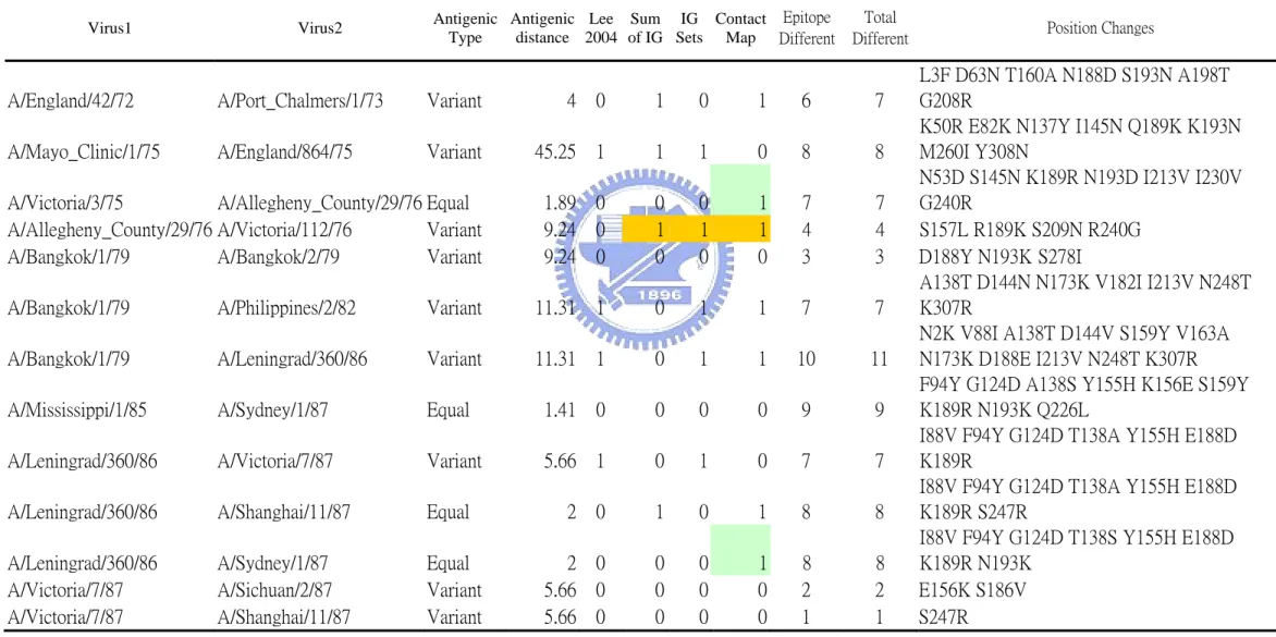
(6) List of Tables Table 1.. The influenza vaccine component recommended by WHO ································31. Table 2.. The six HAI titer tables adapted in training set ···················································32. Table 3.. The list of influenza virus strains in training set ·················································33. Table 4.. The sequence number and name of the 11 clusters in the test set ························34. Table 5.. The residues with top 10 information gain and residues with top 10 codon diversity. ···············································································35. Table 6.. 14 Cases successfully predicted by information gain ··········································36. Table 7.. Analysis the 91 cases predicted by contact map ··················································37. Table 8.. The comparison between our methods and related works ·····································38. Table 9.. The false predicted cases by three methods ··························································39. Table 10. The comparison between our models and related works. ···································42. Table 11. The Detail Information of 50 cases on Test Set1 ·················································43 Table 12. The result of apply training model on test set 2 ····················································44 Table 13. Analysis the rules and positions lead to cluster transitions ··································47 Table 14. Cluster-difference amino acid substitutions, and distances between antigenic clusters ··················································································47 Table 15. This list of all the 39 cases appear both in training set and test set2 ····················48. V.

(7) List of Figures Figure 1. Viruses Recommended for Inclusion in the Influenza H3N2 Virus Vaccines,1968-2000 ·····························································································50 Figure 2. The 3D structure of HA monomer ······································································51 Figure 3. The Hemagglutination Inhibition Test Table ······················································52 Figure 4. The Flowchart of This Research ·········································································53 Figure 5. The Antigenic Map of Influenza A(H3N2) Virus from 1968 to 2003 ··················54 Figure 6. How the Antigenic Type in Application Set is Defined ·······································55 Figure 7. The Flowchart of Processing Query Sequences from ISD ··································56 Figure 8. How the Position-Specific Changes and Contact Map Coding Works ················57 Figure 9. How the Antigenic Distance is Calculated ··························································58 Figure 10. How to Find Immunodominant Positions via Calculation of Information Gain ··59 Figure 11. The Entropy of All 329 Positions ········································································60 Figure 12. The Information Gain of All 329 Positions ·························································61 Figure 13. The Information Gain for 329 Positions Plot on the HA Protein Structure············62 Figure 14. Evaluate Each Position’s Importance via Entropy and Information Gain ············63 Figure 15. The Relation between Information Gain and Genetic Evolution ·························64 Figure 16. The Relation between information Gain and Antigenic Distance ························65 Figure 17. The Ability for Information Gain to Predict Antigenic Variants ··························66 Figure 18. The Advantage of Information Gain than Hamming Distance ····························67 Figure 19. The Flowchart to Select Important Positions with Level Concept ······················68 Figure 20. The change of Information Gain with Levels for the 21 Positions ······················69 Figure 21. The Decision Tree used to Select Important Positions ········································70 Figure 22. The Six Important Positions Selected by Information Gain ································71 Figure 23. The Six Selected Positions and Co-Evolution Positions ·····································72 Figure 24. The Predicting Performance with Different Radius of Contact Map·····················73 VI.

(8) Figure 25. The Decision Tree Generated for Contact Map·····················································74 Figure 26. The Two Co-Evolution Regions Found by Contact Map ······································75 Figure 27. The Information Gain and Sequence Mutations for WER 50 Cases······················76 Figure 28. The Information Gain and Sequence Mutations for 5928 Cases ···························77 Figure 29. The Selected Positions Test on 5928 Cases···························································78. VII.

(9) Chapter 1 Introduction. 1.1 Background Influenza A viruses is a negative-stranded RNA virus which can cause epidemic, is common acute respiratory diseases. And influenza A has the potential to trigger pandemic infection. In Temperate Zone, influenza affected 1%-5% human population. Children were infected most easily, but the infected elders were at the highest risk of complication and death. In industrialized countries, influenza epidemics induced severe damages in economics. Each million people shared social cost of 10-60 million US dollars ([1]). Shortly, prevention and therapy of influenza are very important issues in medicine.. 1.2 Motivations and Purposes Since influenza A virus cause such important epidemic and economic impacts to human beings. The prevention of influenza virus has significant importance. Current strategy for prevention influenza virus is vaccination ([2]). The vaccination with the inactivated influenza vaccines can provide protection when the vaccine strain vaccine antigens and circulating strains share a high degree of similarity in antigenic property of hemagglutinin (HA) protein. But gradual mutations to the HA gene continually produce immunologically distinct strains.. 1.

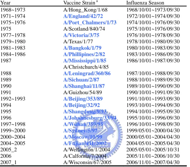
(10) Immune responses from infection by one influenza virus may not protect fully against antigenic or genetic variants of the same subtype (influenza A viruses). As a consequence, influenza outbreaks could occur every year. New influenza vaccine strain must be selected annually to match the circulating viruses. In order to help the selection of future vaccine candidate, to understanding and predicting the antigenic and genetic evolution pattern of the surface antigen HA are desired. Currently there are abundant sequences data and HI titer values which are available from public databases. By the means of analyzing HA sequences and HI titers, we want to answer the important question: which amino acid positions change would have significant effects on host immune response in predicted HI titer values. In other words we want to build relationships between genetic and antigenic evolution.. 1.3 Hemagglutinin and Epitope The two surface glycoproteins Hemagglutinin (HA) and neuraminidase (NA) on the influenza virus are the most important targets for the human immune system [3]. Gradually mutations of HA gene produce immunologically distinct strains of the virus that cause annual epidemic outbreaks. Since the HA are the surface protein of influenza virus, HA is the key component of current influenza vaccine ([1]). From 1968 to 2006 the vaccine component have 22 times of changes (Fig. 1) (Table 1) .The HA protein consists of two chains, HA1 and HA2,. 2.

(11) respectively 329 and 175 residues long. Mostly works focus on the HA1, which is the immunogenic part of HA. The protein 3D structure of HA is determined and deposit in PDB (ex: 1HGF). There are 15 different subtypes of HAs among avian, which need HI test to be identified. The definition of Epitope is the particular site within a macromolecule to which a specific antibody binds . Since HA is surface antigen protein of influenza virus, the epitope to which antibody binds is important to the immune system. Since the protein structure is determined and deposit in the PDB (Ex 1HGF 1KEN). The epitope sites could be determined. There are five epitope sites (A B C D E) contain 131 residues in the full HA1 329 residues [4, 5]. These five antigenic sites show structure clusters in the 3D space (Figure 2).. 1.4 Hemagglutination Inhibition Test The purpose of this test is to determine the function of serum antibody to inhibit the abilities for hemagglutination of flu virus. In the WHO Influenza manual [6], this test can be used to identify influenza isolates since there are 15 different subtype of HA among avian if one uses standardized HA antibody. After a serial HI tests, the result often record in a HI table (Figure 3). The list of first row represents different antisera and the list of first column represents antigen. The value in the table means number folds of dilution. If the value. 3.

(12) between antisera A and antigen b is 320 (Figure 3), that means after a 320 folds serial dilution the antisera still can completely inhibit the hemagglutination. The HI test is extremely reliable [6], provided reference antisera are available to all subtypes. Disadvantages of the HI test include the need to remove nonspecific inhibitors which naturally occur in sera, to standardize antigen each time a test is performed, and the need for specialized expertise in reading the results of the test. However, the HI assay remains the test of choice for WHO global influenza surveillance.. 1.5 Related Works The final purpose of all the influenza researches hope to answer the following questions: when to update vaccine? and how to choose future vaccine candidate [1]? To the purpose, there are many approaches to answer these two questions. Either from experiment or computational approach, scientists collect abundant data and want to discover the pattern or evolution trend of the influenza virus [7-10]. In the view of whether they considering HI titer value, they could be classified into two approaches. First kind of approach focus on the genetic evolution of HA protein [8, 9], and the second kind combine experiment data which could further consider the antigenic evolution of the HA protein [11, 12]. In the genetic level, there had been discovered that those sites of HA1 involved in antigen determination exhibit significantly more non-synonymous nucleotide substitutions. 4.

(13) than synonymous substitutions [8], whereas the remaining sites show the more common pattern of primarily synonymous variation. These observations demonstrate that HA is undergoing positive Darwinian selection for new antigenic variants [13]. Bush et al. [8] have identified 18 HA1 codon sites with significantly higher non-synonymous to synonymous ratios. In order to analysis the evolutional pattern of influenza virus, there had been propose a cluster method [10], which cluster 560 HA protein sequences into 174 clusters. According to the cluster result, there are several representative clusters. By the means of compare genetic variation between intra and inter of representative clusters, they found some evolution trend of influenza virus. They also proposed a method to predict the future vaccine candidate. Before the year of 2004, mostly works focus on the genetic level on HA. Until the year of 2004, there began to have more efforts made on the comparison between genetic and antigenic evolution. The result shows that gradual genetic evolution, but punctuated antigenic evolution [11]. As a result they found that the genetic evolution could not directly correspond to antigenic evolution. Genetic change sometimes had a disproportionately large antigenic effect. The next question should be what are the relations between genetic and antigenic evolution. By collect historical WHO vaccine HI titer tables and HA sequence from 1968 to 2002, a global prediction model is build [12]. The highest performance model for predict antigenic. 5.

(14) variant shows that when there are more than 7 amino acid changes on the epitope sites then a antigenic variant strain is predicted (agreement = 83%). But the importance of these positions in terms of affecting cross-reactive antibody is unclear. In order to find what key position changes would affect cross-reactive antibody interaction. We apply an index value from information theory. The information gain evaluates the relation between two variables (genetic and antigenic evolution). Here we take information gain as a index to represent relations between genetic and antigenic evolution. We hope to find out antigenically important positions and to understand the pattern between genetic and antigenic evolution.. 6.

(15) Chapter 2 Materials and Methods. 2.1 Overview of Research Steps The research flowchart could be divided into two parts (Fig 4). In the first part we calculate the information gain of 329 HA positions from on a representative training dataset and evaluate the fitness for information gain to represent the relations between genetic and antigenic evolutions. Then in the second part we apply the important positions selected by information gain to predict antigenic variants on two unseen and meaningful application sets (test sets). In the first part we first select a representative training set which was used in a published work [12]. Then we extract features from sequences and HA protein structure. The HI titers are transformed from folds of serial dilution to an antigenic distance between two influenza viruses. The large antigenic distance means more antigenic difference between two viruses. After we have two variables (genetic features and antigenic distance), we could calculate information gain for each 329 HA positions. By a well-known method (Decision Tree C4.5) based on information gain we could select several clusters of important positions and get a training model for predicting antigenic variants. After we found important positions, we discuss the fitness for information gain to represent the relations between genetic and. 7.

(16) antigenic evolutions. Those selected positions are then used to predict antigenic variants and compare predicting performance to related works. In the second part we find two unseen test sets which have antigenic properties. The first smaller set (51 cases) were all vaccine strains extracted from WER (1968~2006) and each case with known HI titer value. The second larger set (5928 cases) containing 181 influenza viruses from 1968 to 2003 which having an antigenic clustering label [11]. Then we apply the position and rules from training model on these two test sets. In the following part we would first show that how materials are prepared and then the detail of methods.. 2.2 Influenza Sequence Database The influenza sequence database [14] is a well-known and frequently cited database, which collect the nucleotide sequence of influenza virus. They collect all 3 influenza species and 8 protein segments of various hosts (Appendix ). This difference between NCBI database the ISD is that ISD deposit not only publish sequence but also un-publish sequences. The ISD also provide some useful information such as vaccine selection from 1999 to 2006 (Appendix I) and influenza virus activity in United States from 1981 to now (Appendix I) .Since all sequence is presented in nucleotide format, the translation is required. The EBI translation tool is recommended (http://www.ebi.ac.uk/emboss/transeq/).. 8.

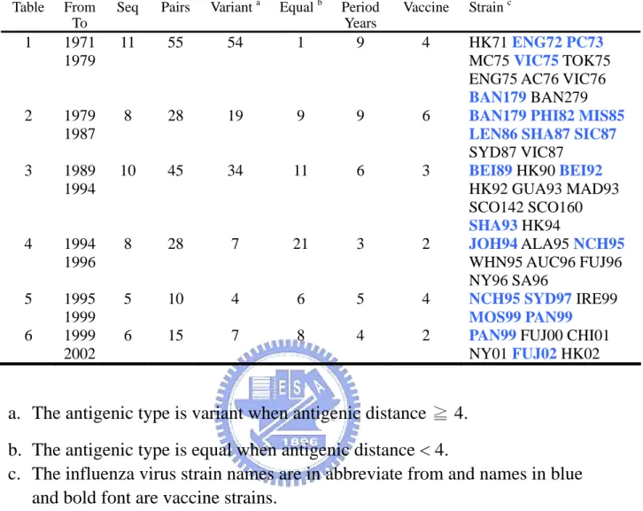
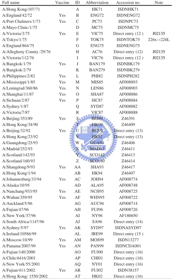
(17) 2.3 Training Set We need a representative and robust training set which should including representative influenza virus strain and the set should better to be complete and balanced. From the literature search we choose a set which was used in a related work [12]. This set consisted of six sets ferret serum HI cross-reactivity data which including 45 influenza virus strains and 181 pairwise ferret serum HI titers (Table 2). From 1968 to 2005 there were 21 influenza virus strains treat as WHO vaccine component (Table 1), and this set cover 17 virus strains of them. The first set included 11 viruses (55 pairwise comparisons, virus ID: A to K) isolated from 1971 to 1979 [15]. The second set included 8 viruses (28 pairwise comparisons, virus ID: J, L to R) isolated from 1979 to 1987 [16]. The third set included 10 viruses (45 pairwise comparisons, virus ID: S to AB) isolated from 1989 to 1994 [17]. The fourth set included 8 viruses (28 pairwise comparisons, virus ID: AC to AJ) isolated from 1994 to 1996 [18]. The fifth set included 5 viruses (10 pairwise comparisons, virus ID: AE, AK to AN) isolated from 1995 to 1999 [19]. The sixth set included 6 viruses (15 pairwise comparisons, virus ID: AN to AT) isolated from 1999 to 2002 [20]. ( Note : the strain TOK75’s position 226 x is assign to amino acid Leucine, which is identical to other residue in table one. The sequence need manually key in table one is using template J02135 ). The information of all the sequences is listed on table 3. After the feature extraction and calculation of antigenic distance, the training set have. 9.

(18) 181 cases and 125 of them are variant type (antigenic distance ≧ 4) while the other 56 cases are equal type(antigenic distance ＜ 4) . Among all the 329 residues of HA protein, there are 101 positions have occurred change in this set.. 2.4 Test Set The purpose of test set is to evaluate the correctness of the positions and rules learning from the training set. Since our method integration both genetic and antigenic evolution, the test set should also containing antigenic property. The first set was extracted from WER (1968~2006), from which we could found 62 reference pairs of HI titer value with both homologous and heterologous titer values and available HA sequences. We further filter these 62 cases with one more criterion: there should have at lease one vaccine strain for the pair comparison. Finally we could got 50 cases satisfy the condition. The second dataset includes 253 sequences. All 253 sequences were grouped into 11 groups according to the K-mean result which using antigenic distances transform from HI titer [11] (Fig 5). After a simple all pairwise comparison, we identify 181 non-identical sequences treated in the test set (Table 4). Since the cluster result were based on antigenic data, we assume that two different cluster would have different antigenic properties (consider as variant) and members within a cluster would have similar antigenic properties (consider as. 10.

(19) equal ) (Fig 6). According to the article, there are 273 isolates .But according to the final grouped table on the supporting material, there are only 253 sequences. According to the query condition in reference and supporting material we could get 255 sequences, but there are 3 sequences of A/SP/1/96(AY661200 AY661199 AY661198) and 1 outlier Dk/33/80. The three A/SP/1/96 sequences in which two are identical, and we adapt the first one AY661200. There is one sequence in the grouped table but not in the supporting material, which is A/Sydney/5/97. So the sequence number : 255-2(two identical)-1(Dk/33/80)+1(A/Sydney/5/97)=253 sequences. The test set have 181 non-identical sequences. After the antigenic type assign, there are 2118 equal cases and 3810 variant cases.. 2.5 The ISD set This set was downloaded from Influenza Sequence Database at 2005/07/10. The query is “ A type, HA, Human, H3” , so we could get 1744 sequences . The sequences download from ISD are in the nucleotide format and the length are not identical, so we need to translate them into protein sequence and modify their length to 329 residues. The flowchart is in recorded (Fig. 7). For some virus strains the isolation date is recorded, so those sequences could be clustered according to the influenza season.. 11.

(20) 2.6 Feature extraction from HA sequence and 3D protein structure. The inputs of this question are two influenza virus strain’s HA protein sequence, then a pairwise comparison is generated. The most common method to compare two influenza virus strains is hamming distance (HD) which counts the total number of changed amino acids [12]. But the HD method can’t explain each position’s different importance to determine antigenic property. We here apply the position-specific change (PSC) coding, the change of each position is independently recorded as a feature (Fig 8). For example, the number of changed amino acids between A/Panama/2007/99 and A/Fujian/411/2002 is 13 positions, so the HD is 13. But the position change method individually record which 13 positions are changed (Fig 8A). Since the protein structure of HA is determined and deposit in the Protein Data Bank [21], we further want to utilities the information of structure environment to find important regions on HA structure. Here we apply the contact map coding which could consider each position’s environment information. In the contact map coding, each position is considered as the center of a sphere (Fig 8B). The region here is defined as a sphere which center at each amino acid position. Since there are 329 positions in HA, there are 329 regions on the 3D structure of HA. If any position in a region is changes, then this region is considered as changed. The radius of the sphere region is test on the training set from 3 to 12 Å to determine what distance’s performance is best. 12.

(21) 2.7 Antigenic Distance We want to find out what positions change would affect HI titer value, so we need to define to what degree the HI titer value is considered as changed. In this work, we divide the degree of HI value difference into two categories: antigenic variant and antigenic equal cases. The HI value from experiment was not convenient for analysis, so the HI values are usually transformed to antigenic distance for large scale analysis. We apply the equation used in the related work [12, 22, 23] to define antigenic variants. This equation calculate the antigenic distance between two virus strains and the equation is show as follows:. (homologous I_I)(homologous J_J) (heterologous J_I)(heterologous I_J). (1). This equation need four cell of HI values that means both two antisera are needed for cross test. A antigenic variant is defined when antigenic distance is ≧ 4. That means both two homologous and heterologous HI test should have HI difference equal or more than 4 times. The example is illustrated in (figure 9).. 13.

(22) 2.8 Entropy Entropy is used to measure the degree of disorder of one space. We use the entropy here to evaluate the disorder of each position as an index in the genetic level. The equation to calculate entropy is as follows:. 20. H ( X ) = − ∑ P r log( P r ). (2). r =1. The H(X) is the entropy of position X and Pr is the probability the amino acid type r in this position. The entropy of position X sums all 20 types of amino acids. The higher the entropy means that position have more genetic diversity.. 2.9 Information Gain Information gain is an index value from information theory with statically meaning. Information gain measures the association between two variables. The higher the information gain means more association between two variables. In this case, a position with very high information gain means if that position is changed then an antigenic variant is expected. As a consequence we could use information gain to build relations between genetic and antigenic evolutions.. 14.

(23) Here we use the information gain to measure the degree of each position change’s effect to antigenic change. The information gain of a given attribute X with respect to the class attribute Y is the reduction in uncertainty about the value of Y when we know the value of X. The equation is show as follows:. I(Y, X) = H(Y) - H(Y | X). (3). The uncertainty about the value of Y is measured by its entropy, H(Y ). The uncertainty about the value of Y when we know the value of X is given by the conditional entropy of Y given X, H(Y |X). Equation (3) could translated into following form:. I(Y, X) = H(Y) -. | YV | H( Y V ) ∑ V∈Value(X) | Y |. (4). Equation (4) works when Y and X are discrete variables that take values in {y1...yk} and {x1...xl}.. 15.

(24) 2.10 Selecting Important Positions by Information Gain The key idea for selecting important positions is as follows: Suppose there are many possible HA mutation patterns for influenza virus to escape immune-selection. So we could classify those different HA mutations into several groups. Each group of mutations could explain part of antigenic change from 1968 to 2002. The process is illustrated in figure (Figure 18). We adapt the greedy method to select important positions. In the level 1 we have full training dataset (181 cases) and then we select the position P1 with highest antigenic association (highest information gain). Those cases in the level 1 which have mutation on P1 is considered as explained by position P1 and those explained cases are removed from the original dataset. Then in the level 2, the non-explained cases all have no mutation on P1, so we find the position P2 with highest information gain for the remain cases in level 2. By recursively selecting positions with highest information gain and then remove explained cases, we could finally find several positions to explain all cases. Decision tree are sophisticated data mining tools for discovering patterns and using them to make predictions. The kernel methodology of decision tree is information gain. Here we adapt the decision tree C4.5 [24] help us to select positions with highest information gain in each levels.. 16.

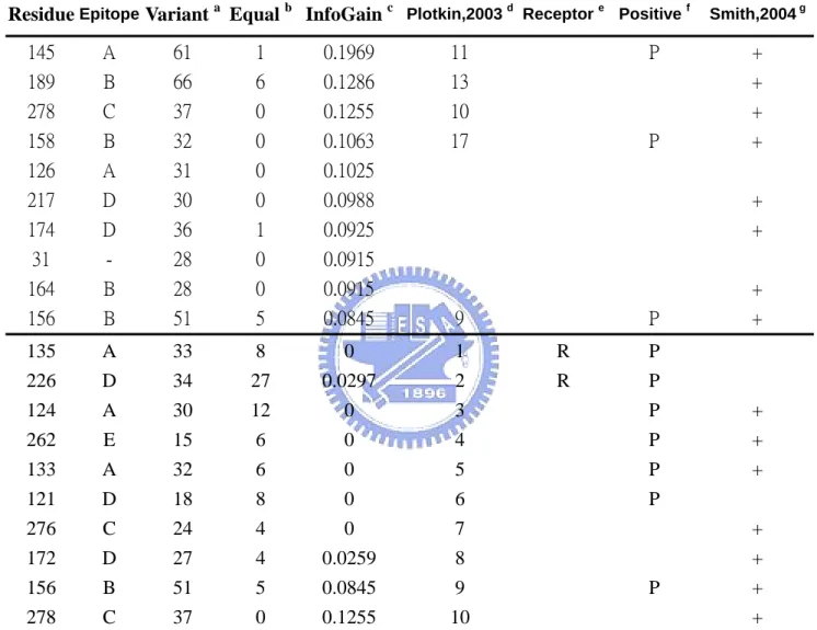
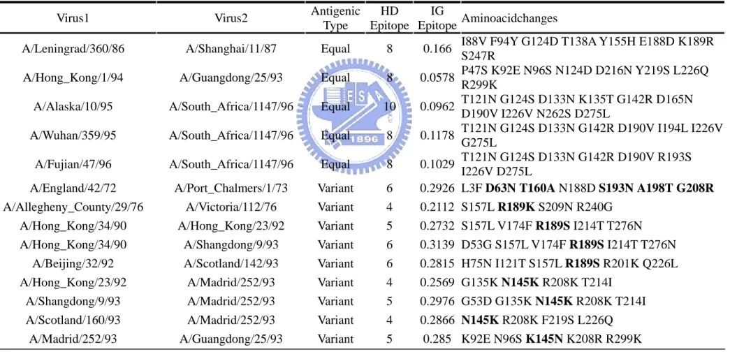
(25) Chapter 3 Results and Discussions. The Results could be divided into two main parts. First part is the evaluation process for the suitability of information gain to represent genetic and antigenic evolution. This part also shows the process and result of selecting important positions via information gain. Second part use the important positions selected by information gain to predict two unseen test set. The predicting performance and results are discussed.. 3.1 The result and meaning of information gain value In order to find out what position change would affect HI value. We calculate the information gain of 329 HA positions from 181 cases. We first to evaluate that whether information gain is a proper index for represent the association between genetic and antigenic evolutions. The process is illustrated in (figure10). In the figure 10 (table A) we list eight cases of virus comparison, the left most column record the antigenic type between that two virus and the right most column record the genetic changed positions between that two virus’s HA protein sequence. In the (table B), we statistic each 329 position’s change frequency in the total 181 cases. The change frequency of one position is separated classified into two. 17.

(26) categories, the change happened in variant type and in equal type. In the (table C), we do the calculation of entropy and information gain for each 329 positions. The top three information gain positions are 145, 189, 278 all have high association with antigenic type. For example, position 145 have total 62 frequencies of change is total 181 cases and 61 of them happened in the variant type. We may conclude that position with high information gain means high association between position change and antigenic type change. The three positions with high entropy are 226, 135, 124 show low association between genetic and antigenic relationship. For example, position 226 have total 61 frequencies of change in total 181 cases and 34 of them happened in variant type and 27 of them happened in equal type. The result shows that position 226 with very low association between genetic and antigenic relations. Specially note the position 145 with top information gain have been verified by experiment that could lead to cluster transition [11]. . The information gain of each position is plot in graph (Fig. 11).The entropy of each position is plot in graph (Fig. 12). We also plot the information gain on the HA structure (Figure 13). Figure 13 shows the information gain for 329 positions on the HA protein structure in the form of color. The red the color means more high the information gain and the top five information gain positions are labeled. Figure (A) is the front view of HA monomer. Figure (B) is the top view of HA trimer. Compare the red region between front view and top view shows that the top view show more high information gain positions. 18.

(27) The comparison between information gain and entropy is also plot in graph (Fig 14). In the genetic view, residues with high entropy may be important. But from the view of information gain, positions with high entropy may have zero information (Ex: position 124). From this figure we may conclude that positions with highest information gain means high association between genetic and antigenic evolutions. The top 10 information gain and top 10 codon diversity positions are list in table (Table 5). The information gain of all positions are listed in appendix ( Appendix II).. 3.2 The Discuss for Information Gain Since information gain associates genetic and antigenic evolution. We here to discuss the relationship between them. The relation between information gain and genetic evolution is plot in figure (Figure 15). For each 181 cases, we compare the genetic changes and information gain for both All positions (329 positions) and epitope sites (131 positions). The linear regression R factor shows good relation between genetic change and information gain (R > 0.9) and epitope sites could better fit the genetic change. But for the same value of information gain, the genetic sequence may have high diversity change. For example the information gain value near 0.5, the position change number could range from 7 to 19. The result shows that information gain treat each position change with different weight, but not equal weight.. 19.

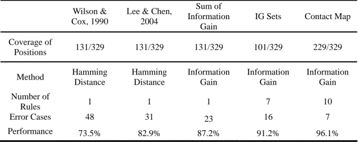
(28) The relation between information gain and antigenic distance is plot in figure (Figure 16). For each 181 cases, we compare the antigenic distance and information gain for both All positions (329 positions) and epitope sites (131 positions). The result shows that sum of information gain could fit the linear relation to antigenic distance (R >0.74). The result also shows that epitope could better fit the antigenic distance than all positions. Antigenic variants are defined when antigenic distance ≧ 4, from this figure when sum of information gain > 0.1835 , we could get best predicting performance for predicting antigenic variant. The agreement is 87%.. 3.3 The Ability for Information Gain to Predict Antigenic Variants From figure 15 we found that information gain have the potential to predict antigenic variants. For each pair of viruses we calculate the sum of information gain of changed positions. And the result is compared with a related work [12] which based on hamming distance (The sum of different amino acid positions). The result is illustrated in figure (Figure 17). For each 181 cases, the information gain and number of sequence mutations of epitope sites is plot on the figure. When the sum of Information gain value > 0.1835, the case is predicted as antigenic variant and the agreement is 87 % (158/181). When the sum of sequence mutations ≧ 7, the case is predicted as antigenic variant and the agreement is 83% (150/181). The different predicted cases are illustrated in figure 18.. 20.

(29) Figure 18 further observe the different predicted cases by these two methods. Cases successfully predicted by information gain but false predicted by hamming distance are label with big circle. The cases in the circle A means little sequence mutations but which leads to antigenic variant pair. The cases in circle B means large sequence mutations but still antigenic equal pair. The result show that when sequence mutations are less than 11 positions, the position which actually changes would more important than the amount of total mutations. The detail information of 14 successful predicted cases are list in table 6. Table 6 list the 14 cases successful predicted cases by information gain but false predicted by hamming distance. Eight cases of nine variant cases have changes on the top two information gain positions (145:0.1969 and 189:0.1286). And only the A/England/42/72 vs A/Port_Chalmers/1/73 pair do not have any position with information gain>0.1 but could reach the information gain threshold to antigenic variant at 0.1836. The five equal cases all have change on positions with low information gain.. 3.4 Selecting Important Positions by Information Gain (IG Sets) We divide the 181 cases into several ordered subgroups according the greedy selection method described in the method section. The flowchart is illustrated in figure (Figure 19). We have 181 cases in the initial and then to find the position with highest information gain. Position 145 have the highest information gain in level one, so the first selected position. 21.

(30) is position 145. There are 62 cases in level one have position changes on 145, so those 62 cases are considered as explained by position 145 and removed from the original set. In each level we further consider those positions with information gain > average + 2*standard deviation. In level one there are other 4 positions satisfy the condition. The position 126 and 278 are considered as co-evolution to position 145 because when the 62 cases are removed from the dataset, their information drop significantly in the level two. The position 189 and 158 are considered as independent important positions would not drop information gain when the 62 cases are removed from the dataset. When the 62 cases are removed from the dataset, we use the same method to select the position with highest information gain in level two. We further illustrate the detail method to select important positions and define co-evolution sites in figure (Figure 20). This figure plots the information gain in 6 levels of the 21 positions selected by information gain. In each level the selected position having the highest information gain. Positions with close information gain behavior are consider co-evolution groups are colored in the same color. For example the first group includes position 145, 278 and 126 are in green color. Specially note that when the position with highest information gain is selected and those cases have mutation on that position is removed from the dataset. The information of that selected position would drops to zero. As a consequence, some positions ( Ex: 155) do not have high information gain in the level one but. 22.

(31) it’s information gain gradually increase from level one to level four. Decision tree tool could help us to select positions with highest information gain for each level in a easy way. The result is illustrated in figure (Figure 21). Figure (A) is the decision tree model of using decision tree tool C4.5 to select the positions with highest information gain. The nodes of decision tree are the positions with highest information gain in each level. The root is on the top of the tree and we should read the tree begin from root. The condition “145 > 0 : Variant (62/1)” means that when position 145 changes and the predicting type is variant. There are 62 cases have change on position 145 and 61 of them are variant type and only one cases disobey the rule. When position 145 have no change (145<=0), then go to check the next position 189. Figure (B) show the selected positions with highest information gain in each levels and the co-evolution positions with that selected position. The last three columns denote the biology meaning and related work’s remark of that selected position. The positions selected by information gain are label on the HA protein structure (Figure 22). The co-evolution positions in each level are also label on HA structure (Figure 23). From the structure view, the co-evolutions all locate on at least two epitope sites. This result match Wilson’s conclusion for drift variant of epidemiologic importance. All positions in 6 levels with top information gain are selected to build a model for predicting antigenic variants, the name of this model is “” IG Sets”.. 23.

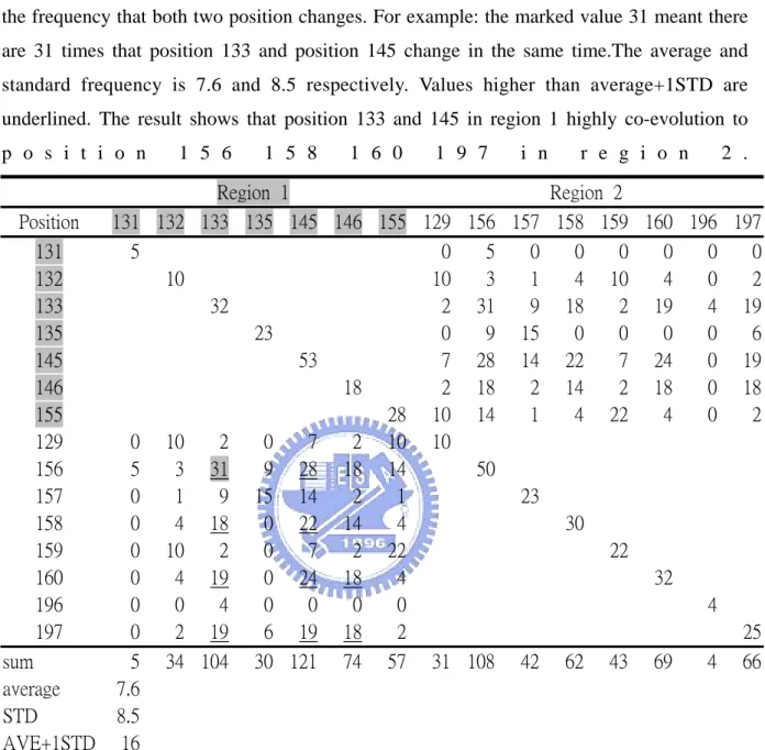
(32) 3.5 The result of Contact Map In the contact map coding, the HA protein structure is divided into many regions which form a sphere center at each amino acid position. The radius of the sphere is tested from 3Å to 12Å and to see which radius’s performance of predicting antigenic variants is best. The test is performed by decision tree and the results are illustrated in figure (Figure 24). According the result we choose radius at 9Å Figure 25 show the positions selected in contact map coding. .Figure (A) Each node in the tree represents a region. Figure (B) The center of each region is list in the table. Position label with “T” means have position change on this set. (C) There are 102 residues covered by all selected regions and 54 of them are in the five epitope sites. Specially note the first rule : when region 160 and region 134 both occur changes then 90 cases of total 91 cases lead to antigenic change, in which this rule match Wilson’s conclusion for drift variant of epidemiologic importance.[5]. This rule imply am important co-evolution relation between this two regions. We further analysis the 91 cases apply the rule found in contact map. The result is at table 7. This table analysis the 91 cases apply the relation found by contact map. The positions are divided into two groups according to structure neighbors. The value represent the frequency that both two position changes. For example: the marked value 31 meant there are 31 times that position 133 and position 145 change in the same time. The average and standard. 24.