Gibbons的內部勞動市場十大核心問題（Ten Core Questions） : 以台灣X公司為例

行政院國家科學委員會專題研究計畫 成果報告

Gibbons 的內部勞動市場十大核心問題（Ten Core

Questions） : 以台灣 X 公司為例

中 華 民 國 94 年 11 月 8 日

Opening the Black Box: The Internal Labor

Markets of Company X

Published in Industrial Relations,

October 2005, vol 44(3), pp 659-705.

Ming-Jen Lin*,

Assistant Professor,

Department of Economics,

National Taiwan University

No 21, Hsu Chow Road, Taiper, Taiwan 100

Contact Tel: +886-2235-19641 ext: 463;

e-mail:[email protected].

__________________________________________

* I thank Steve Levitt and Michael Gibbs for their continuous support and insightful comments. I am grateful to the editor, three anonymous referees, Michael Greenstone, Casey Mulligan, Mark Duggan, Jin-Tian Liu, seminar participants at University of Chicago, National Taiwan University, and Academia Sinica for suggestions that greatly improved the paper. The Field Research Grant and the Henry Morgenthau, Jr. Memorial Fund Dissertation Award from the Department of Economics, University of Chicago are also thanked. Of course, all errors remain mine.

1 ABSTRACT

This paper sets out to analyse an internal dataset on a Taiwanese auto dealer employing three distinct types of workers. The effects of jobs and levels are positive on both the salary and bonus equations, albeit smaller under a fixed effects than under OLS; however, when factoring in individual fixed effects, the reductions in the bonus equations are greater than those in the salary equations. With changing economic conditions, any consequent variations are greater in bonuses than in salaries, with the most extreme variations being felt by higher ranking employees than lower level workers.

Promotion premiums between levels are smaller than the average differences in pay, and although wage variations do exist within and between levels, the greater effect is on bonuses rather than salaries. The variations in both salaries and bonuses, defined by the coeffficient variations, are also greater in those years when demand is high, as opposed to years of low demand. Entry and exit behavior is observed at all levels, although it is more likely to occur amongst the lower levels of the hierarchy. Finally, we present strong evidence in support of the cohort effect. Overall, our findings confirm the prevalence of internal labor market theories.

JEL Classification: J3, M5.

2 1. INTRODUCTION

“The best scenario imaginable is that I just sit here doing nothing, and enjoy the profits that my employees earn for me’

CEO of Company X, On the functions of the internal labor market. In neo-classical economics, wages are determined by their marginal value; however, it is difficult to believe that wages are solely determined by spot markets, since individuals actually spend most of their lives in firms, or internal labor markets. In their seminal work, Doeringer and Piore (1971) set out to fill the gap that existed at that time, by raising the concept of ‘internal labor markets’ (ILMs): “An ILM is an

administrative unit within which the pricing and allocation of labor is governed by a set of administrative rules and procedures. ILMs interact with external labor markets (ELMs) through certain ports of entry or exit, with the remaining jobs within the ILMs being filled by promotions or transfers. In consequence, these jobs are shielded from any direct influence of the ELMs”.

Nevertheless, it is clearly the case that promotions, hierarchies, rules, hidden information and even organizational culture, all have some part to play in ILMs. Although their claims cannot be viewed as theories, Doeringer and Piore’s observations did inspire a wide range of economic theories that attempted to explain what happens inside the firm. The list includes specific human capital (Becker, 1993), authority and control (Rosen, 1982), principal-agent theory (Holmstrom, 1979), learning and matching (Jovanovic, 1979a, 1979b), tournament (Lazear and Rosen, 1981) and institutional design (Lazear, 1979, 1986).1 Gibbons and Waldman (1999b) went on to provide a comprehensive survey of these models, whilst Lazear (1999) even defined research along such lines as ‘personnel economics’, suggesting that:

“personnel economics, defined as the application of labor economics to business issues, has become a major part of economics”.

This area of research does, however, suffer from a scarcity of empirical works, which is why Baker and Holmstrom (1995) claimed that the subject of internal labor markets had “too many theories, and too few facts”. Furthermore, most of the empirical studies tend to be based upon western companies and white collar workers;

1 _{Models mixing at least two of the above elements are Murphy (1986), Prendergast (1993) and}

3

however, as Gibbons (1997) put it, “all four systems (salaried, industrial, craft and

secondary), as systems in other countries, deserve more attention”. Therefore, using

data on blue and white collar workers within a Taiwanese firm, this paper sets out to contribute to the knowledge that has thus far escaped the attention of many researchers in this field.

Although the spirit of this study is very much in line with Baker et al. (1994a, b), because of the uniqueness of the data adopted, our paper contains a lot of new findings. One of the most interesting observations is that, although this is a Taiwanese company heavily influenced by Japanese culture, most of the findings corraborte those contained in the existing literature on the broad patterns generally found in US and European firms. Furthermore, since we have three types of workers and detailed data on salaries and bonuses, we can simultaneously compare six different responses for each question asked. As compared to many of the earlier studies, which have invariably used only managers as observation points, this study also sheds light on the ways in which the differences in work characteristics affect the results.

The remainder of this paper is organized as follows. The next section provides a review of the literature, followed, in Section 3, by a description of the dataset, new methods of identifying the hierarchical structure, and details of transition within the company. Section 4 provides a description of the effects that jobs and levels have upon salaries and bonuses, as well as variations within and between the different levels of the sub-internal labor markets and the model specifications. We also compare the coefficient reductions of wage regressions, for both salaries and bonuses, between OLS estimations and a fixed effects model, as well as wage variations between salaries and bonuses for years of both high and low market demand. Section 5 discusses the existence of ports of entry and exit, followed by an examination of the cohort effect in Section 6. The conclusions drawn from this study are presented in Section 7.

2. LITERATURE REVIEW

A summary of our review of the literature, including the type of firms being studied, the countries involved, the periods covered, the sample workers, the compensation variables used and the main conclusions, is provided in Table 1. Our review focuses primarily on those studies that have used personnel data to investigate the ways in which workers are allocated and priced, the way in which the rewards system (or the

4

human resource management system) affects the behavior of workers, 2 and the ways that ELMs interact with ILMs. As the table shows, 19 of the 28 studies surveyed were undertaken after 1999, which indicates that this is still a relatively young field.

Furthermore, with the exception of one Japanese firm, all of the samples in the prior studies are taken from western countries (half of them being in the US) demonstrating a distinct lack of studies for comparison in the east. Moreover, only seven of these studies were able to obtain data on the entire workforce, which precludes any overall comparison of the sub-internal labor markets across firms. Most of the samples were either white, male managers, or particular occupational groups, such as installers or claims processors. Finally, only five of the studies have any significant data on bonuses; however, since bonuses are extremely important to employees in company X, especially for salespeople and technicians, a separate exploration of the bonus system may raise some interesting issues.

A point worth mentioning is the nature of the data. Most ILM studies tend to adopt what is essentially a ‘case study’ method, using data on individual firms; one reason for this is the scarcity of national employer-employee matching data. Eriksson (1999), Lima and Pereira (2001), Eriksson and Werwatz (2003) and Lazear and Oyer (2003) are exceptions to this rule, since each of these studies used data on European countries in their entirety. However, whilst data on all of the firms within a single country may be useful in determining the general features of ILMs, data on a single firm still has its own advantages in terms of defining jobs and levels; hence, promotion and demotion, for example, can be more precisely defined. Furthermore, workers in the same firm are also faced with the same personnel policies which critically affect their behavior; in contrast, the use of large-scale data makes it extremely difficult to control for the effects of changes in internal policies even through a fixed effects model. Hence, these two types of data should be seen as complementary to the overall understanding of ILMs.

As to the purposes of the prior studies in this area, some set out to establish the stylized facts of ILMs (Lazear, 1992; Baker et al. 1994a, 1994b; Seltzer and Merret, 2000; Treble et. al., 2001; Gibbs and Hendricks, 2004; Eriksson and Werwatz, 2003; Lazear and Oyer 2003), whilst others focused on more specific issues, such as the relationship between tenure and productivity (Medoff, 1980, 1981; Lazear, 2000;

5

Flabbi and Ichino, 2001; Kwon, 2002), or the effects of changes in compensation methods (Ichniowski et al., 1997; Paarsch and Shearer, 1999; Lazear, 2000). This paper follows similar lines to the Baker et al. (1994a) and Lazear (1992) studies; consequently, the results derived from this data may be viewed as either confirming or contesting the literature, at least from the perspective of other firms and/or cultures.

3. DATA, HIERARCHY AND TRANSITION 3.1 Overview of the Firm

The sample for this study is an auto dealer engaging in the sale and maintenance of automobiles; it has more than ten years history in Taiwan and has a share of the Taiwanese vehicle market in excess of 5 per cent. The period covered by the data is from 1991 to 2000, a period during which there were, on average, around 600-800 people working in the company at any given time, comprising of both white and blue collar workers. The data includes the personal characteristics of each worker, such as age, gender, the number of years and type of education, tenure within the firm, salary and bonuses (both performance-related and profit-share based), as well as details on job codes, levels, performance rating for staff workers, and so on.

Between 1991 and 1996, the company achieved rapid growth in virtually every area; however, after 1996, as a result of the rapidly increasing market competition and the general slowdown in the Taiwanese economy, the company found itself facing a slight decline in overall performance. Figure 1 shows the basic financial conditions of company X, demonstrating around five-fold growth in sales from NT$2 billion in 1991 to NT$9 billion in 1994, and thereafter, a slight decrease from NT$10 billion in 1995 to NT$8 billion in 2000.3 A similar pattern is discernible in employee numbers, up from 300 in 1992 to 1,000 in 1995, then stabilizing at around 850 at 1999. Assets also reached their peak in 1996, whilst net income reached its highest level, of NT$230 million, in 1993, followed by a general decline; there was, however, an apparent recovery in this area from 1999 onwards. An examination of the general features of this growth-decline pattern will be undertaken later in the discussion of the interaction between ELMs and ILMs.

6 3.2 Identifying the Hierarchy

Jobs are used to ‘define’ employees, as well as their level of responsibility and authority within a firm. A hierarchy, according to Baker et al. (1994a), is usually said to “consist of job titles aggregated into levels related to the job’s authority and placed

in the path of decision-making”. Hence the term ‘levels’ can be viewed as the simple

version of ‘jobs’ to define a hierarchy, and transitions between levels can also help us to gain an understanding of the relationship existing between different units within the organization. Hence correctly defining jobs and levels is the cornerstone for any subsequent analysis.

In a prior work, Lazear (1992) used average pay to define levels; however, when undertaking an investigation of the relationship which exists between pay and levels, this is, essentially, an example of tautology. In contrast, Baker et al. (1994a, b) used information on moves between job titles to define levels, selecting fourteen major titles from their dataset (which represented 90 per cent of the sample) and using the transition matrix of these titles to construct the hierarchy, as well as the levels within it. Nevertheless, the major disadvantage of both methods is that the observations on compensation, job titles and transitions are used to infer the structure of the hierarchy, and are thus sensitive both to the errors that can occur during the sampling process, and to the process itself. Baker et al. (1994a) admitted that although they had 4,000 cost center codes, they could not use these as a means of describing the hierarchy because of the unavailability of data on the reporting relationships.

The first contribution of this paper is its use of job titles, levels of authority and the hierarchical structure chart (provided by the company’s HR department) to directly identify job levels.4 This is the first paper to specifically use an organizational chart to identify the hierarchy and, as we will see in the following section, the results confirm, quite strongly, that the Baker et al. method was very effective, despite the fact that they did not have an organizational chart at their disposal. Since there are around 30 job titles in total, we begin by defining the CEO as the highest level, and then trace each level of ‘direct’ authority down to the lowest levels. For example, if documents initiated and reviewed by the Deputy Chief Manager have to pass through the hands of the General Chief Manager before being seen by the CEO, then the hierarchy, and the

4 _{The way in which this company allocates employee’s seats is also a method of identifying levels,}

7

levels defined by authority, would follow the order of CEO, General Chief Manager and then Deputy Chief Manager.

The company’s HR Department also has its own hierarchical chart which provides a representation, in very graphic detail, of the way that the company sees its own organizational structure. Sometimes a job title itself will describe the relationship. By using such readily available information, we are able to quickly construct the hierarchy of the firm, and its levels, as shown in Figure 2. As can be seen from the figure, the CEO and his officers control the company through two sections, Sales and Administration, which are headed by two Assistant Chief Managers.

The administration section has overall responsibility for finances and human re-source management, whilst the most important job for the sales section is to direct product sales by the head of the product department (General Manager) and the area store chiefs (who may have the title of Deputy General Manager or Manager). Below the area stores are the sales branches, whose job it is to promote and sell the products, and the maintenance branches, which are responsible for repairing or maintaining the products sold by them.

There are also three sub-hierarchies within these branches. Bonuses for salespeople are calculated by the number of cars sold, with approximately 80 per cent of a salesperson’s annual compensation being derived from this source. In contrast, only 20 per cent of a staff worker’s annual compensation is derived from bonuses, which are related to the worker’s performance rating. Team and individual incentives are used for technicians, and as a result, about 50 per cent of a technican’s income is derived from group or individual bonuses.

It should be noted, however, that our field survey shows that whilst the reporting rules for staff workers and techinicians are rigid and unambiguous, levels of authority amongst salespeople are more informal,5 particularly between levels 1 and 2; and indeed, two different ranks are sometimes categorized at exactly the same level, simply because their numbers are so small. For example, there was only one level 1 specialist in any given year of the entire 10-year data period. This categorization should not, however, affect our results.

5 _{That is, the sanctions for not obeying a higher level salesperson, comprise of a mix of peer pressure}

8

3.3 Different Transition Paths for Different Workers

Investigating the movement of employees within the internal labor market is another way of gaining an understanding of the hierarchy from a dynamic perspective. Although, in their sample of managers, Baker et al. (1994a) found that demotion rates were rare (less than 0.3 per cent), it is, nevertheless, intuitive to think that different types of workers may have different transition paths due to factors such as the time taken to build up firm-specific human capital, or the preciseness of output measurement. Furthermore, demotions may also be used, in effect, to provide incentives. We go on here to use the dataset to explore this particular issue.

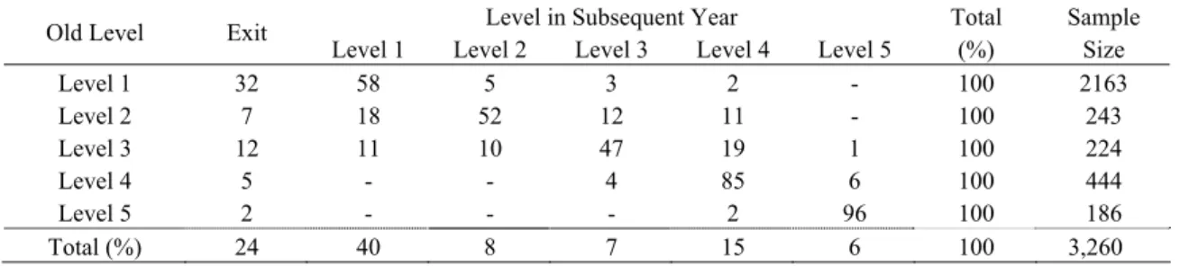
Tables 2-1, 2-2 and 2-3 show the respective transition matrices for the company’s three different types of workers, between 1991 and 2000. We find that the exit rates for level 1 technicians and staff workers were about 20 per cent, whilst around 75 to 89 per cent of these workers remained at the same level in the subsequent year. Promotion rates for these groups were around 3 to 7 per cent, whilst demotion rates were between 0.5 and 2 per cent. In line with the Baker et al. (1994a) findings, the number of demotions amongst these two types of workers was not large.

The most active and significantly different transition path within the company, in terms of both promotion/demotion rates and exit rates, was found amongst salespeople. The probability of a salesperson at level 1 leaving the company in the subsequent year was 32 per cent, as compared to 22 per cent for technicians and 17 per cent for staff workers. Only 50 per cent of salespeople at levels 2 and 3 would remain at the same level in the subsequent year; however, whilst 20 per cent would receive promotions, a similar proportion would be demoted, and 10 per cent would be likely to leave the company; thus, demotions are clearly not so rare amongst salespeople. It should also be noted that we calculated the transition rates for those remaining with the firm between the good (1991-1995) and bad (1996-2000) years, and found no differences, which indicates that the firm uses relative, rather than absolute, performance standards to evaluate its employees.6

Why do these transition paths differ so much? The simple answer is that the promotion rules are written into the company’s personnel books; each salesperson undergoes a review every three months, and his or her level is determined, routinely, on the basis of performance (i.e., the number of cars sold). Thus, if they continually

9

fail to perform well, senior salespeople can quite easily be demoted to level A within 6 months. The rapid transition rates also indicate that the reporting relationships between salespeople from levels 1 to 3 are more informal than those for other types of workers.

Such personnel policies result in the emergence of an extremely wide-ranging transition path between different types of workers, which gives rise to a very interesting question; i.e., what is the economic intuition behind these rules? In general, promotion serves more than one purpose, since it includes the provision of additional incentives, it sends out signals to third parties, and brings with it on-the-job training, placement and screening (Waldman 1984); hence the rate of promotion may also be related to these factors. On the provision of incentives, Lazear (1986) highlighted the conditions whereby a firm should use higher power incentive schemes (such as piece rates, as opposed to fixed salaries). The work of a salesperson seems to fall into line with every aspect of this theory; it is easy to measure the salesperson’s output; errors in output measurement are extremely low, monitoring costs are high (a deputy manager cannot follow a salesperson every working day); and workers are less homogeneous (selling products to people requires charm, which is sometimes regarded as a talent that cannot be taught). Since higher compensation, including internal and external status, usually comes with promotion, a rapid promotion system would provide stronger incentives because the immediate value of the expected return for each car sold would be that much higher. Staff workers, on the other hand, are at the opposite end of the scale; it is extremely difficult to measure their output, both in qualitative and quantitative terms; hence, errors in output measurement will be high. It will therefore take longer to judge such workers’ abilities, which inevitably results in a slower promotion/demotion incentive scheme.

To summarize this section, we have aimed to provide an overall definition of jobs and the hierarchy of the company. As the transition matrix shows, most people will stay at the same level in the subsequent year and there are some promotions and demotions, although, with the exception of salespeople, occurrences of the latter are rare. It is, however, clear that transition paths are quite different across different types of workers. Whilst 20 per cent of salespeople will experience promotion in the subsequent year, a similar proportion will also experience demotion; this is a direct result of the personnel policies of the company and the special characteristics of the work of its salespeople. Some economic intuition is provided in order to explain this phenomenon, but it may well be that in the future, a formal model will be required.

10 4. JOBS, LEVELS AND PAY

One of the important features of the Doeringer and Piore (1971) study was that wages in ILMs were determined by an administrative process rather than by the spot market, and hence were attached to jobs or levels. In fact, a number of empirical studies (including Baker et al. 1994a, b; Treble et. al., 2001; Grund, 2002; and Kwon, 2002) have found that levels and jobs are strongly correlated to wages. Tournament theory (Lazear and Rosen, 1981), scale of operation effects (Rosen 1982), levels as a proxy to sort ability (Gibbs 1995), or inducing human capital (Prendergast 1993), are theories that are often used to explain this phenomenon. Although this evidence seems to support Doeringer and Piore’s argument, at the same time, almost every study on ILMs finds that there are substantial pay variations, both within and between levels (Baker et al. 1994a; Treble et. al., 2001; Grund, 2002; Kwon, 2002; and Gibbs and Hendrick 2004). If wages are only decided by levels or jobs, then we have clear evidence on ILMs since they are not affected by the conditions of ELMs. Furthermore, if there are variations within and between levels, and these variations vary across different years, then the effects of the spot markets may also be coming into play. However, Gibbs and Hendricks (2004) found that whilst wage variations existed between levels, the wages of those who were not promoted were, in the long run, attached to their jobs. The following discussion aims to probe these phenomena.

4.1 Salaries, Bonuses and Jobs

Most of the prior studies have used levels to estimate the relationship between hierarchy and compensation; one exception was Seltzer and Merrett (2000) which, using job codes as the unit of analysis, demonstrated that job dummies had an effect on wages. Since we have clear job codes, we can also undertake a direct comparison of the coefficients of job dummies in order to determine whether wages are attached to jobs; he first task here, however, is to adequately define compensation.

The compensation of employees within firms in Taiwan generally comprises of four parts: (i) salaries, which are the basis of all compensation and which are dependent on both the job itself and tenure; (ii) performance bonuses, which are dependent on worker performance, based, for example, on the number of items a salesperson can sell (iii) year-end bonuses, which represent the traditional form of bonus schemes in Taiwan, and are paid on 16th December of the lunar calendar – these

11

usually comprise of around one-and-a-half to three months salary and are adjusted both by tenure and an individual’s performance measure for that year; and (iv) profit sharing, where 1 or 2 per cent of a company’s post-tax profits may be distributed to its employees, according to their job level and seniority; however, this does not usually take place each year.

Although Lazear (1992) and Baker et al. (1994a) used only salaries (the fixed element of earnings) as their object for analysis, bonuses are, nevertheless, becoming increasingly important. For example, in the company under examination in this study, 80 per cent of the total compensation for a typical salesperson, and 40 to 50 per cent of the total compensation for a technician was derived from performance bonuses. This paper therefore uses salaries and bonuses [bonus = (ii) + (iii) + (iv)] as the basic units of analysis for compensation, under the following model specifications:

ln (Earnings ijt) = β0 + β1.j*Jobit + β2 Education Dummies ijt

+ β3* Male +β4 Tenure + β5* Tenure2 + β6*Year Dummies (1)

+ β7*Performance Dummies (staff workers only) + Eijt

where i is the individual; j is the job code dummy; Tenure and its square indicate

years worked with the firm; and year dummies are used to exclude the economy-wide shock. This is the Mincer specification used in Baker et al. (1994a), Card (1999), Gibbs and Hendricks (2004) and many other papers within the literature. The dependent variables used in this study are compensation, salaries and bonuses. In order to correct the unobserved time invariant variable bias and serial correlation, we adopt the following employee fixed effects AR(1) model:

ln (Earnings ijt) = β0 + β1.j*Jobit + β2 Education Dummies ijt

+ β3*μi +β4 Tenure + β5* Tenure2 + β6*Year Dummies (2)

+ β7*Performance Dummies (staff workers only) + Eijt

where Eijt=Uijt + Pi*Uij(t-1) . Model specification (2) indicates that, in addition to

the employee fixed effects μi, the error terms of the last period also affect the

dependent variable, with the effect of Pi being different for different individuals. The main point of interest here, of course, is to see whether all β1j should be included in

12

the model (the F value of the exclusion test), and whether β1j is different across

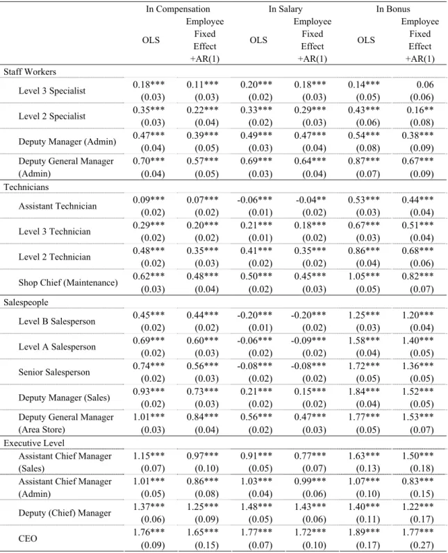
different jobs. The results are shown in Table 3-1. Note that the total number of job titles used in the regression is 17, as opposed to the 30 mentioned earlier; this comes as a result of the combination of some of the job titles with very few observations.

The first thing we can see is that the F-value of the exclusion test is very large, indicating that job dummies are a valid set of independent variables. Furthermore, almost every coefficient is significant. In the OLS model, for example, based upon a comparison with an assistant specialist, the annual total compensation for a level 2 specialist is 29 per cent higher, whilst the total compensation for a level 2 technician is 42 per cent higher, and that of a level A salesperson is 62 per cent higher. We can also see that the coefficients increase with rank within different types of worker groups. Some of the coefficients in the bonus and salary regressions for the salespeople group are negative, because, in absolute terms, salespeople typically receive very low salaries; by far, the greatest proportion of their compensation (80 per cent) is derived from bonuses. Hence, it is possible that in absolute terms, the salary of a level A salesperson could be smaller than that of a staff worker (the comparison group in Table 3-1); indeed, the larger number of coefficients in the bonus columns for the sales group confirms this point. To some extent, this corresponds with the point made by Lazear (1998) that the firm “sells the jobs” to its salespeople. We also find that the employee fixed effects AR (1) model produces similar to the OLS estimations, albeit with generally slightly smaller coefficients.

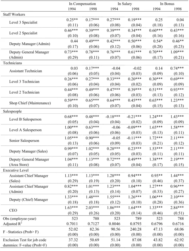
Another interesting approach would be to see whether changes in the overall economic conditions would bring about greater variations in earnings for some jobs than for others. In good years versus bad years, for example, the CEO’s bonus may vary significantly more than the bonuses received by other employees. Hence, we run the OLS regressions for 1994 (the highest sales value, which represents a good year) and 1998 (the lowest sales value, which represents a bad year); the results are presented in Table 3-2.

We find that the variations in salary across different jobs, represented by the differences in job-code coefficients between good and bad years, were quite limited. For example, the CEO coefficients in the salary equations for 1994 and 1998 were 1.86 and 1.64, respectively, indicating a 20 per cent decrease. For level 2 technicians, the corresponding numbers were 0.47 and 0.39, indicating a 15 per cent drop. There

13

were, however, substantial differences between the good and bad year coefficients within the bonus equations. For example, the CEO coefficients in the 1994 and 1998 bonus equations were 1.33 and 2.84, respectively, indicating a 110 per cent increase. For level 2 technicians, the corresponding numbers were 0.51 and 0.93, indicating a 90 per cent increase.

We also found that the variations in the bonus equations were greater for executive level employees than for lower level staff workers and salespeople. For example, the 1994 and 1998 Deputy Chief Manager coefficients for 1994 and 1998 were 1.06 and 2.10, respectively, indicating a 100 per cent increase, whilst the corresponding numbers for senior salespeople were 1.72 and 2.11, indicating a 17 per cent increase. To summarize, when economic conditions change, workers experience greater variations in bonuses than salaries, with the greater variations being felt amongst higher ranking employees than lower level staff workers and salespeople. Overall, the evidence points to differences in remuneration for different jobs, irrespective of whether this is measured in terms of total compensation, fixed salaries or bonuses.

Finally, we also ran a fixed effects AR(1) regression to dispose of the unobserved time invariant variables and to correct any serial correlation errors. The results show that whilst the coefficients of job titles are still significant, they are significantly weakened. With a change in economic conditions, the greatest variations are felt in terms of bonuses rather than salaries, with higher ranking employees experiencing greater variations than lower level staff workers and salespeople. The variation is also greater in the bonus equations than in the salary equations; we shall explore this issue later, together with the equation results for different worker levels.

4.2 Correlation Between Salaries, Bonus and Levels

In order to further investigate the relationship between pay and hierarchy, we categorize job codes into level variables and run:

In Salary(Bonus) ijt = β0 + β1.j*Levelit + β2 Education Dummies ijt

+ β3* Male +β4 Tenure + β5* Tenure2 + β6*Year Dummies + β7 *Type (3)

14

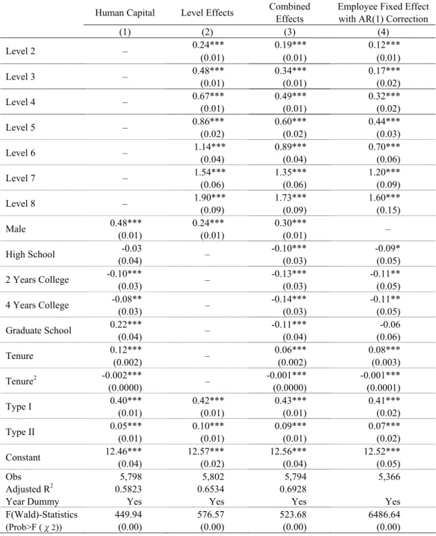
The compensation regression results for the different specifications are presented in Table 4. The procedure and the results here are basically the same as those presented in Table 3-1 and in equations (1) and (2), with the exception that the job dummies are now replaced by level dummies. The employee fixed effects AR (1) model results (with employee-specific error term structure) are also reported, with the findings indicating that levels are positively correlated to compensation across different specifications, and that the coefficient of the employee fixed effects AR (1) model is again, positive, albeit smaller. The results and conclusions drawn are thus similar to those in Table 3-1. One phenomenon, which also occurs in Table 3-1, is the small, but negative, effect of education. This non-intuitive result may be due to some of the education coefficients being obtained after controlling for levels. If education is positively related to levels (that is, education affects wages mainly through levels), we may detect an insignificant, or even negative, effect of education on earnings.

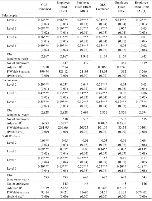
Running all workers and pay within one regression has its advantages, since all workers come under one general personnel rule; however, since this company has three types of workers, one might argue that there are actually three sub-internal labor markets within our dataset. It may also be useful to check whether different levels have different effects on salaries and bonuses. Here we use ‘log bonus’ and ‘log salary’ as the dependent variables, and separate the samples by the different types of workers. The specifications include OLS estimations and the employee fixed effects model with AR(1) corrections, in similar vein to equation (3). The results are presented in Table 5. For the purpose of brevity, we report only the coefficients of levels, although all the other independent variables are included. We find that when using the employee fixed effects model with AR(1) corrections, both the salary and bonus equations for salespeople and technician levels have a positive but smaller effect than the OLS model. The results for staff workers are also similar; however, the positive relationship between levels and bonuses is weakened. These results are basically consistent with the Eriksson (1999) and Seltzer and Merrett (2000) findings, and can be interpreted from the perspective of individual heterogeneity; higher level employees were paid more due to both their higher abilities and the policy of attaching higher wages to higher levels.

We also arrive at the same conclusion with the employee fixed effects AR(1) model with job codes as the independent variables (Table 3-1), and total compensation

15

as the dependent variables (Table 4). The reduced effect brought about by adding in the individual fixed effects is, however, greater in the bonus equations than in the salary equations. The salary of a level 3 technician, for example, is 47 per cent higher than a level 1 worker in the OLS (combined) model, but only 11 per cent higher in the fixed effects model; however, in the bonus equation, the same employee earns 47 per cent more in the OLS model, but only 6 per cent more (which is, in fact, insignificant) in the fixed effects model.

For staff workers, however, after controlling for human capital variables, or after using the fixed effects AR(1) models, explanatory power seems strong only at the higher levels. Overall, this suggests that cross-sectional variations between salaries for different levels cannot be explained by the predetermined differences between them, at least for staff workers, which contradicts the argument of Piore and Dorengier (1971) that “wages are attached to jobs or levels”. It is also clear that human capital theory has its own role to play in the wage regressions.

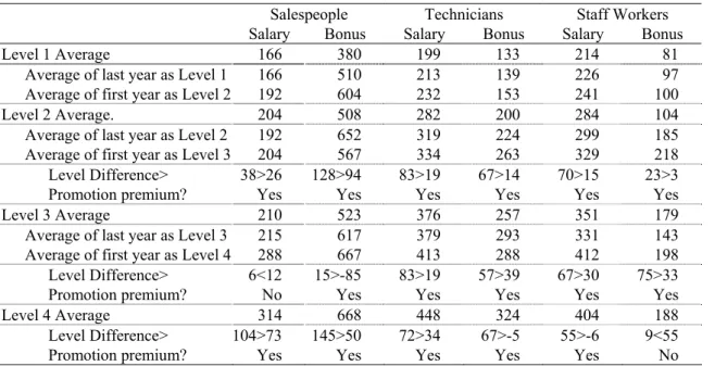
When the fixed effects model is used, the effects of levels can only be identified by those moving up or down within the hierarchy; the reduction of the effects of levels from the OLS model to the fixed effects model (presented in Tables 3-1, 4 and 5) is also consistent with the finding that pay increases based upon promotion are smaller than the average differences in pay between levels, one of the ten core questions on ILMs for which, according to Gibbons (1997), empirical researchers should provide evidence. In order to investigate this argument more directly, we can simply compare the average growth in wages, based upon promotion, to the differences in mean wages for adjacent levels.

Table 6 presents the promotion premium and the mean wage difference between levels across the different types of workes. We can see, for example, that the average level 1 salesperson earns a salary of NT$166,000, which is the same as the previous year’s salary for a level 1 salesperson; however, in his first year as a level 2 salesperson, his salary would raise to NT$192,000, despite the average salary for a level 2 salesperson being NT$204,000. We can see, therefore, that the promotion premium (26) within a salesperson’s salary, is less than the average difference between adjacent levels (38); indeed, of the 18 comparisons calculated, 16 support this claim.

Our data supports the argument that pay increases based upon promotion are smaller than the average difference in pay between levels. This result is as predicted by

16

the Gibbons and Waldman (1999a) study, which developed a model to intergrate job assignments, human capital acquisition and learning. Promotion, in their model, came from the accumulation of effective ability. In the case of full information or symmetric learning, the average higher level workers, who were much older, had accumulated much more human capital than lower level workers. Their model also implied that unobserved talent was positively correlated with job levels, with the more talented workers invariably ending up in the higher job levels. Nevertheless, promotion could only capture “one year of the wage difference”, hence the difference in average wages between two adjacent levels was greater than the average wage increase based upon promotion.

The evidence presented here, which distinguishes between salaries and bonuses, sheds new light on these issues; indeed the evidence presented on the differences between salaries and bonuses essentially suggests that, largely as a result of administrative rules, salaries are more rigid than bonuses. Presumably, bonuses are more likely to reflect short-term incentives or product market considerations, whereas salaries are more likely to reflect long-term considerations, such as a worker’s accumulated effective ability.

As mentioned earlier, variations within and between levels are also important in testing the hypothesis that “wages are attached to jobs”. In order to determine whether there are actually wage variations within and between levels, and whether these variations are different across different types and years, we plot the fifth, fiftieth and ninety-fifth percentile salaries and bonuses of salespeople, technicians and staff workers, by levels, for the years 1995 and 2000. Figures 3-1 to 3-6 illustrate these results. The immediate impression gained is of a positive correlation between salaries (the dotted lines) and levels, with the one exception of the medium salary figure for level 2 to level 3 salespeople in 1995. As to bonuses, the relationship is generally positive, with the occasional odd deviation (for example, the drop in bonuses between levels 3 and 4, but only for the ninety-fifth percentile of staff worker in 2000). These features, shown by the raw data, are consistent with the regression results.

4.3 Variations Within and Between Levels

As to the variation within and between levels, we can see that salaries and bonuses both have some degree of variation across both years and types of workers. For

17

example, in 2000, the salary range between the fifth percentile and the ninety-fifth percentile for salespeople at levels 2 and 3 were almost identical. The salary level at the ninety-fifth percentile for a level 2 salesperson is about 50 per cent higher than his fifth percentile colleague. In 1995, the salary and bonuses for a fiftieth percentile level 3 staff worker were even greater than those of a corresponding counterpart at level 4.

For most cases, however, a ninety-fifth percentile lower level worker earns more than an upper level fiftieth percentile worker, whilst the salary and bonuses of ninety-fifth percentile workers are also around 50 per cent to 200 percent greater than their fifth percentile colleagues at the same level. We can also find that the variations in bonuses, both within and between levels, are significantly greater than those of salaries across different years, different type of workers, or different levels. We can therefore argue that variations within and between levels do exist, and that these are greater for bonuses than for salaries.

A further interesting method of approach, with regard to verifying the existence of ILMs, would be to compare the scale of the variations between years of positive growth and years of decline; this is undertaken by investigating the ways in which external economic conditions have an effect upon wage policies within the firm. We use here, as a normalized standard, the coefficient of variance (CV), which is equal to standard divided by mean, in order to compare the amount of variation across levels, pay variables and different types of workers. Table 7 tabulates the results. Across the same types of workers, levels and pay variables, we find a persistent pattern of CVs in 2000 (a year of decline) being smaller than in 1995 (a growth year). For example, the CV for bonuses for a level 2 salesperson in 1995 is 0.21, but in 2000, the number falls to 0.10. We also see that the CV for salaries for a level 2 staff worker in 1995 was 0.07, but in 2000, the number falls to 0.02, representing a 70 per cent drop.

The only exception is the comparison of bonuses for staff workers. Hence, the firm does undertake adjustments to its salary and bonus structures, for any given levels and types of workers, in response to changes in external conditions. This corresponds with the results of the ‘implicit contract story’ in Beaudry and DiNardo (1991). Furthermore, the size of the CV for bonuses is greater than that for salaries across different levels and types of workers, similar to the findings of Gibbs and Hendricks (2004), and consistent with our findings presented in Figures 3-1 to 3-6. It seems, therefore, that market demand, and hence, external market conditions, do impact upon

18

the internal labor market through both salaries and bonuses, and that bonuses are more sensitive in their response than salaries. The whole picture suggests that, at least in this firm, workers are not completely shielded by the ILMs, and that the level of such shielding is different across different market conditions and pay variables.

We find that the overall effects on the salary and bonus equations, for both jobs and levels, are positive and smaller under a fixed effects model than under an OLS (combined) model; however, when adding in the individual fixed effects, the reductions are greater in the bonus equations than in the salary equations. The latter result, together with a direct calculation of the promotion premium and the mean wage difference in adjacent levels, provides support for one of the ‘ten core questions’ posed by Gibbons (1997), that pay increases based upon promotion are smaller than the average differences in pay between different levels. Wage variations do exist, both within and between levels, and they are larger for bonuses than for salaries. Furthermore, the variations in both salaries and bonuses, defined by the coeffficient variations, are greater in those years when demand is high, than in those years when demand is low. The last of these findings is new to the literature, and may require further theoretical investigation in the future.

5. PORTS OF ENTRY AND EXIT

According to Doeringer and Piore (1971), workers enter or leave a firm through ports of entry and exit, with incumbents having priority with regard to internal promotion,7 and indeed, this is an important element with regard to providing support for the existence of ILMs. It may be that job matching and learning theories can also provide support for this statement. Jovanovic (1979a) found that a worker’s inherent abilities are revealed in gradual steps, over time, hence a ‘stayer’ realizes that there is no need to quit and to have to start looking once again for another match. Jovanovic (1979b), found that if the information revealed about a worker was sufficiently positive, the worker would invest a greater amount of firm-specific human capital into the company, and thus, would succeed in gaining promotion; if the reverse was true, the worker would leave. Both models imply that high frequency matching (entry and exit) should occur in the lower levels of the firm since opportunities for leaving at a higher level are smaller. Becker’s specific human capital theory can also be used here. If the human capital possessed by workers is rather

19

general in nature, then the cost of leaving will be small, even though they may be in the higher levels of the company. Hence ports of entry should exist when human capital is more firm-specific. Baker et al. (1994a) and Hamilton and MacKinnon (2001) each interpreted their finding on the basis of this argument.

We therefore examine, in this section, whether these issues are apparent within our dataset, with Figures 4-1 and 4-2 providing details of the firm’s new hiring rates and the exit rates for all employees, by levels and years. Two properties are immediately clear. First of all, there are occurrences of entry and exit in all four levels investigated. Secondly, levels are, in general, negatively associated with entry and exit rates. Overall, from 1993 to 2000, the new hiring rates went from 50 per cent to 30 per cent for level 1; from 40 per cent to 12 per cent for level 2; from 20 per cent to 2 per cent for level 3; and from 5 per cent to 2 per cent for level 4. The same pattern is also discernible in the figures for exit rates. Between 1994 and 2000, the exit rate was around 30 per cent to 40 per cent for level 1, and around 20-25 per cent lower than the new hiring rate for level 2, at around 10 to 15 per cent. The exit rate was around 5 per cent to 10 per cent for levels 3 and 4, quite a bit higher than the new hiring rate.

The existence of entry and exit ports can be further investigated across the three sub-samples. Table 8 provides the entry and exit rates, recorded by years and types of workers, for the two periods, 1991-1995 (growth), and 1996-2000 (decline). The first impression is that entry and exit occurs in levels 1 to 3 across different type of workers; however, for technicians and staff workers, entry and exit rates decrease with levels. For example, the respective entry rates for technicians at levels 1, 2 and 3, were 0.27, 0.26 and 0.04, whilst their exit rates were 0.19, 0.09 and 0.03. The respective entry rates for staff workers at levels 1, 2 and 3, were 0.28, 0.26 and 0.06, whilst their exit rates were 0.15, 0.12 and 0.01. This can be explained by both learning and matching theory and human capital theory; higher level workers are either better matched to the firm, or, as time goes by, they simply gain more firm-specific human capital. We also find higher entry and exit rates for salespeople at level 1; however, the entry and exit rates for these workers are greater at level 3 than at level 2.

To summarize, in this section we have argued that although entry and exit is observed at all levels, it is more likely to occur in the lower levels of the hierarchy for all three types of workers. This suggests that with an increase in levels, workers represent a good match with the firm, and possess more firm-specific human capital.

20

6. THE EXISTENCE OF THE COHORT EFFECT

As pointed out in Mason and Fienberg (1985), cohorts are categorized by their idiosyncratic life experiences, in terms of say, labor market or educational experiences. The use of cohorts refers to “groups defined by a point of entry into the social system”. Those belonging to a large cohort, or those entering university after the 1968 student movement, for example, are expected to be different from other cohorts. The cohort effect also plays an important role in the context of the internal labor market, and is again categorized as one of the ‘ten core questions’ by Gibbons (1997).

According to Gibbs and Hendricks (2004), one of the most fundamental debates in the literature on ILMs is whether personnel policies have any real effect, or whether they are just a ‘veil’ through which the pressures of the external labor market act relatively unimpeded. In order to distinguish this issue, one needs to investigate the ways in which the internal labor market conditions, or the spot labor market conditions, affect workers’ wages. Such an analysis should involve individual-level data, rather than aggregate-level data, in order to avoid any potential bias resulting from changes in the composition of the workforce.

The economic intuition justifying the existence of the cohort effect in ILMs is evident in two studies. Firstly, Beaudry and DiNardo (1991) argued that, starting from the time of a worker’s entry, and under the assumption of simple implicit contracts, the history of the market conditions (whether these be market wages or unemployment rates), would maintain its effect, because that was the point when the employees and the employer signed their contract. There would, therefore, be a cohort effect in existence. If it was the spot market condition that dictated the employee’s wages through the veil of the internal labor markets, then the cohort effect would not exist. Secondly, an alternative theoretical justification for the existence of the cohort effect can be seen in Gibbons and Waldman (2003) where they extended their earlier model (Gibbons and Waldman, 1999a) by the addition of two further assumptions; first of all, that the economy can be good or bad, and secondly, that human capital is task-specific, rather than firm-specific, with some element of a worker’s acquired human capital going under-utilized at the time of their promotion. 8 They argued that “a cohort hired

8 _{Task-specific human capital is, as suggested, specific to the task being performed. This is also}

closely related to Adam Smith’s idea that ‘learning by doing’ at the level of the task is an important source of increased productivity.

21

in a bad state has low average wages years later…[this] is because the proportions of workers who start at low level jobs will affect the numbers, and productivity, of workers in high level jobs, years later”. What is even more interesting is that the model does not need to assume friction, as in the Beaudry and DiNardo (1991) study, since it works even under a spot market setup.

The prior empirical literature also provides support for the existence of the cohort effect. Using unemployment rates as the key factor in the cohort effect, Beaudry and DiNardo (1991) found that prior market conditions, together with current market conditions, also affected current wages, and thereby, the implicit contract theory; hence, providing support for the cohort effect. Baker et al. (1994b) used cohort effect dummies to determine all of the relevant variables that would affect wages through the unique cohort experience and found that the cohort effect was highly non-linear: “as it should be, if it reflects external labor conditions”. More recent studies (including Kown, 2002; and Gibbs and Hendricks, 2004) have also investigated the cohort effect, and indeed, our aim in this paper is to reveal a much clearer picture of the existence of the cohort effect since our dataset contains two pay variables for three different types of workers. Note that we focus on identifying the importance of the entire cohort dummies as a set of wage determinants, rather than the significance of any single coefficient, for reasons which we will explain later.

In order to investigate the existence of the cohort effect, we begin by modifying equation (3), simply by the addition of cohort dummies, and by replacing tenure within the firm, and its square, by tenure dummies:9

ln salary(bonus) ijt = β0 + β1.j*Levelit + β2 Education Dummies ijt

+ β3* Male + β4 Tenure dummies + β5* Cohort Dummies (4)

+ β6*Year Dummies + β7 *Type Dummies + Eijt

Theoretically, β4 ,β5 and β6 respectively represent the effects of human capital,

particular cohort experience and economic shock. Our interest would presumably rely upon the interpretation of β5; however, as pointed out by Mason and Frienberg (1985), Heckman and Robb (1985) and Baker et al. (1994b), this specification is actually the

9 _{Our emphasis in this section is purely on the existence of the cohort effect, per se; we do not try to}

22

famous Cohort-Tenure-Year (CTY) problem. Whilst the use of tenure, cohort and year can exist independently, since tenure (three years in the firm) = year (2000) – cohort (entering in 1997) it therefore produces an exact linear relationship between the three. In consequence, no unique solution can exist for the OLS estimations; that is, there are many sets of β4, β5 and β6 that solve the equations, therefore, any individual

interpretation of any β5 would be meaningless. Without further restrictions, it is impossible to separate the effects of cohort, tenure and year; we therefore refrain from identifying the individual coefficients here.

Fortunately, however, the CTY problem can be mitigated, if not solved, by various strategies. In this section, we will apply several of the techniques presented in the earlier literature to tackle the CTY problem. Note that six different matches of worker types and pay will be regressed for each of these methods.

The first solution involves verification only of the existence of the individual coefficient, rather than attempting to assess its economic significance. Indeed, it has been argued that, even without determining the ultimate solution, important conclusions can still be drawn, since: “the question is whether or not we can reject the null hypothesis that all cohort effects are zero” (Baker et al., 1994b; p.935). Using this strategy, and after controlling for tenure and year effects stemming from the high F statistics of the exclusion test, both Baker et al. (1994b) and Gibbs and Hendrick (2004) found that the addition of a cohort dummy into the regression significantly affected salaries over time. Thus, both studies verified the importance of the cohort effect. However, a limit to this approach is that the cohort coefficient patterns may be of some interest, since they may be related to business cycle variables.

The second strategy for a solution to the CTY problem was suggested by Mason and Fienberg (1985), and involved limiting any one of the three parameters to zero. A significant number of the earlier studies have assumed that only two of the three variables will affect the outcome (e.g., Glenn and Davis, 1988; Glenn, 1994). Kennedy (2003) also suggested that one way of solving the problem of multi-collinearity was to drop one set of variables since, by so doing, we can obtain meaningful economic cohort coefficients. However, this process should be based on theoretical reasoning, not data. Since human capital theory predicts that working experience leads to increases in both productivity and wages (factors which have been widely verified empirically), and since the cohort effect coefficients are the estimates on which we are

23

concentrating here, dropping the year dummies is our only choice; that is, our test will compare whether, after controlling for all observables, workers with the same numbers of years tenure, but entering the firm at different times, earn different wages.

The third strategy involves breaking down linear independence simply by assuming a non-linear functional form of tenure. In order to check for sensitivity, we use the square, cubic and quartic of tenure within the regressions. As Baker et al. (1994b) demonstrated, we can also compare those regressions which use different functional forms of tenure against those regressions which use tenure dummies, to determine whether or not tenure has a linear, or quartic effect on wages.

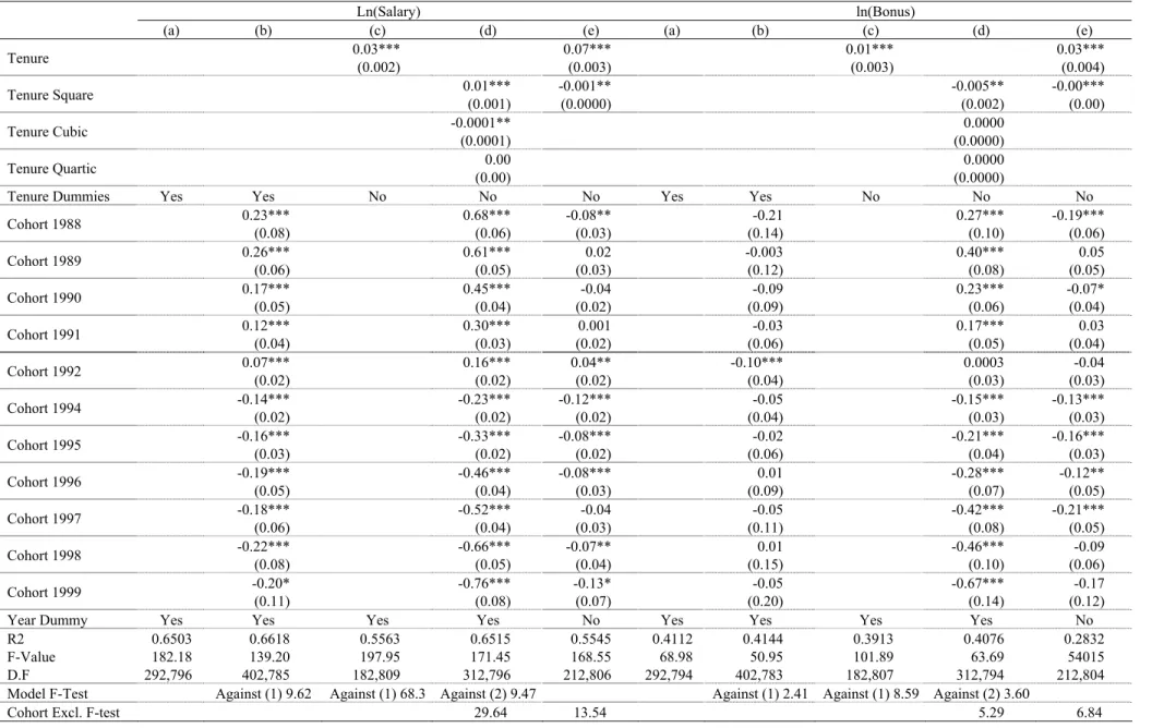
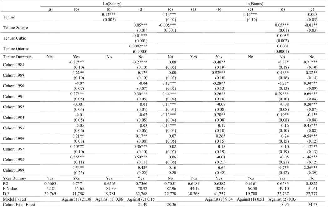
The 30 regressions presented in Table 9-1 to 9-3 provide the results of the three strategies outlined above. We now use the salary regressions on salespeople as an example to illustrate our test procedure, first of all running equation (4) with and without cohort dummies (specifications a and b), and then using the exclusion test to see whether the cohort effect should be included within the regressions. The F-statistic obtained by testing specification (b) against specification (a) is 24.34, indicating that the cohort dummies as a whole, represent significant determinants of the salary of a salesperson. This is the procedure for the first of the three strategies mentioned above.

For the second strategy, specification (c) is the same as (a), except that the tenure dummies are now replaced by a linear tenure variable. The F-statistic of specification (c) tested against (a) is 2.38, which suggest that the tenure effect is not linear.10

For the third strategy, we again use equation (4), this time replacing the tenure dummies with tenure square, cubic and quartic, so as to avoid the identification problem in specification (d). We find that four out of the eleven cohort coefficients are significant.11 However, one might argue that the significance of the cohort dummies comes merely from the arbitrary selection of the comparison group; therefore, we also report the cohort dummy exclusion F test value (= 24.51), which again supports the existence of the cohort effect. We also test specification (d) against (b), which gives an F-statistic of 0.24, indicating that the tenure quartic function is sufficiently representative of the tenure dummies. The tenure effect within this specification is concave and reaches its peak at around 12 years. Specification (e) estimates the cohort effect by simply dropping the year dummies, which corresponds to the second strategy, where we compared whether those

10 _{A test to determine whether or not the tenure effect was linear was also reported in Baker et al. (1994b;}

3rd last line of p.935,.

24

workers with the same number of years tenure, but who had entered the firm at different times, earned different wages. Again the cohort dummies’ exclusion F test value was 15.2, which also provides evidence to support the existence of the cohort effect.

Now we can apply the same interpretation above to investigate all of the six type-pay matches. First of all, we find that cohort dummies are significant determinants for all types of workers and pay variables. The respective F statistics for the six type-pay matches (b against a) are 24.35, 3.87, 9.62, 2.41, 21.38 and 9.04. All of these passed the critical F exclusion test value at the 1 per cent level.12 _{The large cohort dummy}

exclusion F test values for specification (d) and (e) also verify the existence, importance and non-linearity of the cohort effect. Baker et al. (1994b) were concerned that the cohort effect might simply be due to changes in the composition of entrants, thus they ran the regression on entry wages only with the human capital and year dummies. In their test for whether the year dummies represented a set of meaningful dependant variables they concluded that this was not the case, since they found a 22.97 F-statistic.We ran the same specification, and found that the respective F statistics for the six type-pay matches were 17.83, 11.25, 12.21, 26.41, 4.90 and 14.61, which supports the Baker et al. (1994b) findings.

Another interesting issue is the determination of whether a limited number of tenure variables is sufficient to pick up all of the tenure dummy effects. We can see that for staff workers, linear tenure, or the functional form which contains its square, cubic and quartic terms, provides a sufficient approximation of the tenure effect. The same conclusion can be drawn for the salaries of both technicians and salespeople, but not for their bonuses. This finding contradicts the observations of Baker et al. (1994b), that linear tenure is a good proxy for the tenure effect. Finally, by comparing the size and significance of the coefficients, we can see that there is a weaker cohort effect amongst salespeople that amongst other workers. This is consistent with the evidence provided earlier that salespeople have higher rates of demotion, and that most of their compensation comes from bonuses, which ties them more directly to their market value. Overall, we have confirmed that there is strong evidence supporting the existence of the cohort effect, similar to many of the findings in the prior literature, and that this effect is not driven by the composition of the entrants.

25 7. CONCLUSIONS

This study has presented an analysis of the internal labor economics of a Taiwanese auto dealer, Company X, comprising of three different sub-internal labor markets, salespeople, technicians and staff workers. We have offered evidence on ILMs from the perspective of another culture, and have therefore attempted to render these stylized facts more reliable and universal. Our empirical results are similar to those of Baker et al. (1994a, b), providing mixed evidence on Doeringer and Piore (1971).

Using job title, authority level and the structural hierarchy of the company to identify the various levels, we find significant differences in the employment transition paths across the different types of workers. We argue that the effects of jobs and levels, on both the salary and the bonus equations, are positive and smaller under a fixed effects model than under an OLS (combined) model; however, when adding in individual fixed effects, the reduction is greater in the bonus equations than in the salary equations. With changes in economic conditions, greater variations occur in bonuses than in salaries, and higher ranking employees feel the effects of these variations more than lower level staff workers and salespeople. Wage variations do exist within and between levels, and they are greater for bonuses than for salaries. Furthermore, the variations for both salaries and bonuses, defined by the coeffficient variations, are greater in the years when demand is high than in years of low demand.Entry and exit is observed at all levels, but this is more likely to occur in the lower levels of the hierarchy. We have also verified the existence of the cohort effect, and find that it is not driven by the composition of the entrants.

Our evidence shows that the external and internal markets are both working, and that ILMs can only partially shield workers. Furthermore, a very interesting finding is that although this is a Taiwanese company, heavily influenced by Japanese culture, most of the findings corraborte the earlier literature, in terms of the broad patterns found in US and European firms, which suggests that ILMs work in a more general setting.

The dataset has demonstrated a number of interesting comparisons with the stylized facts of ILMs. Through the concepts of the internal hierarchy, levels, ports of entry and exit, and the relationship between salaries, bonuses, jobs and levels, we have verified the existence of sets of rules and procedures that effectively define the internal labor markets. It is hoped that the findings of this study will provide some contribution to the ongoing quest of many economists for the opening up of ‘the black box of the internal economics of the firm’.

26 REFERENCES

Ariga, Kenn, Giorgio Brunello, and Yasushi Ohkusa (1999), ‘Fast Track: is it in the Genes? The Promotion Policy of a Large Japanese Firm’, Journal of Economic Behavior and

Organization, 38(4): 385-402.

Baker, George, Michael J. Gibbs, and Bengt R. Holmstrom (1994a), ‘The Internal Economics of The Firm: Evidence From Personnel Data’, Quarterly Journal of Economics, 109(4): 881-919. Baker, George, Michael J. Gibbs, and Bengt R. Holmstrom (1994b), ‘The Wage Policy of a Firm:

Evidence From Personal Data’, Quarterly Journal of Economics, 109(4): 921-55.

Baker, George, and Bengt R. Holmstrom (1995), ‘Internal Labor Markets: Too Many Theories, Too Few Facts’, American Economic Review, 85(2): 255-9.

Beaudry, Paul, and John DiNardo (1991) ‘The Effect of Implicit Contracts on the Movement of Wages over the Business Cycle’, Journal of Political Economy, 99(4): 665-88.

Becker, Gary S. (1993), Human Capital: A Theoretical and Empirical Analysis, with Special

Reference to Education, 3rd edn., Chicago: University of Chicago Press.

Card David, (1999), ‘The Causal Effect of Education on Earning’, in O Ashenfelter and D Card, eds., Handbook of Labor Economics, Vol. 3, North-Holland, Amsterdam.

Chiappori, Pierre-Andre, Bernard Salanie, and Julie Valentin (1999), ‘Early Starters versus Late Beginners’, Journal of Political Economy, 107(4): 731-60.

Craig, Ben, and John Pencavel (1992), ‘The Behavior of Worker Cooperatives: The Plywood Companies of the Pacific Northwest’, The American Economic Review, 82(5):1083-1105. Doeringer, Peter B., and Michael J. Piore (1971), Internal Labor Markets and Manpower Analysis,

New York: M.E. Sharp.

Dohmen, Thomas J.(2004), ‘Performance, seniority, and wages: formal salary systems and individual earnings profiles’, Labour Economics, 11(6):741-763.

Dohmen, Thomas J., Ben Kriechel and Gerard A. Pfann (2004), ‘Monkey Bars and Ladders: The Importance of Lateral and Vertical Movements in Internal Labor Market’, Journal of

Population economics, 17(2): 193-228.

Eriksson, Tor, (1999), ‘Executive Compensation and Tournament Theory: Empirical Tests on Danish Data’, Journal of Labor Economics, 17(2): 262-80.

Eriksson, Tor, and Axel Werwatz (2003), ‘The Prevalence of Internal Labour Markets – New Evidence from Panel Data’, Working Paper, Aarhus School of Business.

Flabbi, Luca, and Andrea Ichino (2001), ‘Productivity, Seniority and Wages: New Evidence from Personnel Data.’, Labour Economics, 8(3): 359-87.

27

Verbal Ability’, Sociology of Education, 67(3): 216-30.

Glenn, Firebaugh, and Kenneth E. Davis (1988), ‘Trends in Anti-black Prejudice, 1972-1984: Region and Cohort Effect’, The American Journal of Sociology, 94(2): 251-72.

Gibbons, Robert S. (1997), ‘Incentives and Careers in Organizations’, in: D. Kreps and K. Wallis (eds.), Advances in Economics and Econometrics: Theory and Applications, 7th World

Congress, Vol.2, New York: Cambridge University Press.

Gibbons, Robert S., and Michael Waldman (1999a), ‘A Theory of Wage and Promotion Dynamics Inside Firms’, Quarterly Journal of Economics, 114(4): pp 1321-1358.

Gibbons, Robert S., and Michael Waldman (1999b), ‘Careers in organizations: theory and evidence’, in: O. Ashenfelter and D. Card (eds.), Handbook of Labor Economics, Vol.3B, Netherlands: North-Holland.

Gibbons, Robert S., and Michael Waldman (2003), ‘Enriching A Theory of Wage and Promotion Dynamics Inside Firms’, NBER Working Paper 7689.

Gibbs, Michael J. (1995), ‘Incentive Compensation in a Corporate Hierarchy’, Journal of

Accounting and Economics, 19(2): 247-77.

Gibbs, Michael J. (2001), Pay Competitiveness and the Quality of Department of Defense Scientists and Engineers, CA: Rand.

Gibbs, Michael J., and Wallace Hendricks (2004), ‘Are Formal Salary Systems a Veil?’, Industrial

and Labor Relations Review, 58(1): 71-93.

Grund, Christian (2002), ‘The Wage Policy of Firms - Comparative Evidence on the US and Germany from Personnel Data’, Working Paper, University of Bonn.

Hamilton, Barton, and Mary Mackinnon (2001), ‘An Empirical Analysis of Career Dynamics and Internal Labor Markets During the Great Depression’, Working Paper, University of St Louis, Washington.

Heckman, James J., and Richard Robb (1985), ‘Using Longitudinal Data to Estimate Age, Period and Cohort Effects in Earnings Equations’, in W. Masons and S. Fienberg (eds.), Cohort Analysis in Social Research: Beyond the Identification Problem, NY: Springer Verlag.

Howlett, Peter (2001), ‘Careers for the Unskilled in the Great Eastern Railway company, 1870-1913’, London School of Economics: Department of Economic History, Working Paper No.63.

Holmstrom, Bengt R. (1979), ‘Moral Hazard and Observability’, Bell Journal of Economics, (Spring), 10: 74-91.

28

Resource Management Practices on Productivity: A Study of Steel Finishing Lines’,

American Economic Review, 87(3):291-313.

Jovanovic, Boyan (1979a), ‘Job Matching and the Theory of Turnover’, Journal of Political

Economy, 87(5),(Part I): 972-90.

Jovanovic, Boyan (1979b), ‘Turnover and Firm-Specific Human Capital’, Journal of Political

Economy, 87(6): 1246-60.

Kennedy, Peter (2003), A Guide to Econometrics, 5th _{edn., Cambridge, MA: MIT Press.}

Kwon, Illoong (2002), ‘Incentives, Wages and Promotions: Theory and Evidence’, Working Paper, University of Michigan: Department of Economics.

Lambert, Richard A., David F. Larcker and Keith Weigelt (1993), ‘The Structure of Organizational Incentives’, Administrative Science Quarterly, 38: 438-61.

Lazear, Edward P. (1979), ‘Why is there Mandatory Retirement?’, Journal of Political Economy, 87(6): 1261-84.

Lazear, Edward P., and Sherwin Rosen (1981), ‘Rank-Order Tournaments as Optimum Labor Contracts’, Journal of Political Economy, 89(5): 841-64.

Lazear, Edward P. (1986), ‘Salaries and Piece Rates’, Journal of Business, 59(3): 1346-61.

Lazear, Edward P. (1992), ‘The Job as a Concept’, in: W. Burns Jr. (ed.), Performance

Measurement, Evaluation and Incentives, Cambridge, MA: Harvard Business School Press.

Lazear, Edward P. (1998), Personnel Economics for Managers, J.R. Wiley & Sons.

Lazear, Edward P. (1999), ‘Personnel Economics: Past Lessons and Future Directions’, Journal of

Labor Economics, 17(2): 199-236.

Lazear, Edward P. (2000), ‘Performance Pay and Productivity’, American Economic Review, 90(5): 1346-61.

Lazear, Edward P., and Paul Oyer (2003), ‘Internal and External Labor Markets: A Personnel

Economics Approach’, NBER Working Paper No.10192.

Lima, Francisco, and Pedro T. Pereira (2001), ‘Careers and Wage Growth within Large Firms’, Working Paper, Bonn: IZA.

Mason, William M., and Stephen E. Fienberg (eds.), (1985), Cohort Analysis in Social Research:

Beyond the Identification Problem, NY: Springer Verlag.

McCue, Kristin (1996), ‘Promotions and Wage Growth’, Journal of Labor Economics, 14(2): 175-209.

Medoff, James L., and Katharine G. Abraham (1980), ‘Experience, Performance and Earnings’,