Integration of a quantitative feedback theory (OFT)-based active noise canceller and 3D audio processor to headsets

Mingsian R. Bai

e-mail: [email protected]

Jianliang Lin

Department of Mechanical Engineering, National Chiao-Tung University, 1001 Ta-Hsueh Road, Hsin-Chu 300, Taiwan

Integration of a Quantitative

Feedback Theory

_{„QFT…-Based}

Active Noise Canceller and 3D

Audio Processor to Headsets

This paper seeks to enhance the quality of spatial sound reproduction by integrating two advanced signal processing technologies, active noise control (ANC) and three-dimensional (3D) audio, to a headset. The ANC module of the headset is designed based on the quantitative feedback theory (QFT), which is a unified theory that emphasizes the use of feedback for achieving the desired system performance tolerances in the face of plant uncertainties and plant disturbances. Performance, stability, and robustness of the closed-loop system have been taken into account in the loop-shaping procedure within a general framework of the QFT. On the other hand, 3D audio processing algorithms including the head-related-transfer-function and the reverberator are realized on the platform of a fixed-point digital signal processor. Listening tests were conducted to evalu-ate the proposed system in terms of various subjective performance indices. The experi-mental results revealed that the 3D headset is capable of delivering superior rendering quality of localization and spaciousness, with the aid of the ANC module.

关DOI: 10.1115/1.2748461兴

1 Introduction

Three-dimensional共3D兲 audio has emerged as a new technol-ogy to create spatial sound field for a great variety of applications including home theater, multimedia, MP3 player, TV, mobile phones, games, toys, automotive audio, and so forth. However, it frequently occurs that the quality of the sound reproduction can be significantly degraded when the user is exposed to a noisy envi-ronment such as streets, stations, shopping centers, and vehicle cabinets. It is then desirable to develop effective methods to ad-dress the noise problem before the spatial sound reproduction is implemented. Conventional ways of noise abatement are either to isolate or to dampen the noise source or path by using passive elements, e.g., sound-absorbing materials. Despite the simplicity, conventional methods are known to be ineffective at low frequen-cies, where required passive elements can become impractically bulky. Therefore, instead of using passive treatments, active noise control 共ANC兲 techniques are employed in the present work to cope with the disturbing noises especially for those at low fre-quencies. By “active,” we mean to cancel the noise using an elec-tronically created counternoise. Among all ANC applications with varying degree of complexity, active headsets are perhaps the most mature and have achieved great commercial success. Active headsets enable quality sound reproduction with reduced back-ground noise level.

An active headset system is proposed in this paper to enhance the quality of spatial sound reproduction by integrating 3D audio processing and ANC. The ANC module of the headset is designed based on the quantitative feedback theory共QFT兲 关1–3兴, which is a unified theory that emphasizes the use of feedback for achieving the desired system performance tolerances in the face of plant uncertainties and plant disturbances. Performance, stability, and robustness of the closed-loop system have been taken into account

in the loop-shaping procedure within a general framework of the QFT. The feedback controller shall be implemented by using ana-log circuits to avoid unnecessary delay.

The 3D audio processor aims at producing a sensation of local-ization using head related transfer functions 共HRTF兲 关4兴 and a sensation of spaciousness using artificial reverberators. A HRTF is a transformation for a specific source direction relative to the head, which describes the filtering process associated with the diffraction of sound by the torso, head, and pinnae关5–7兴. A sound image in the 3D space can be created with the aid of digital filters that simulate the HRTF at the intended direction. Specifically, the filter is usually implemented as a finite impulse response共FIR兲 filter by using the head-related impulse responses共HRIR兲, or the inverse Fourier transform of the HRTF. Several HRTF databases are currently available关4,8兴. The HRTF database we used for the present work is from the website of the MIT media lab关4兴.

Reverberation results from the endless reflections of sound waves in a bounded space. As another important element of 3D audio, reverberation carries the cues of human perception to acoustic environment such as the size of room and the absorptivity of the boundary. In audio reproduction and mixing, reverberation is necessary for enriching the dry recording to make it sound more natural and spatial than the original. In some ill-conditioned lis-tening environments, e.g., car cabin, artificial reverberation is also useful in mitigating the coloration problems due to a small space during surround presentation. Reverberation can also be used in the context of headphone rendering to externalize the sound im-ages so that listening discomfort can be minimized.

Listening tests are carried out to compare the performance of 3D audio processing, with and without the ANC, in terms of vari-ous subjective indices. The results are post-processed by using the analysis of variance共ANOVA兲 to assess the statistical significance of the results. The comparison will be summarized in terms of computation cost and subjective performance indices.

2 Active Noise Control

2.1 ANC Overview. The origin of the ANC technique dates

back to 1936. It has been an active area in acoustics since Lueg filed his patent关9兴. ANC is sound field modification or cancella-Contributed by the Technical Committee on Vibration and Sound of ASME for

publication in the JOURNAL OF VIBRATION AND ACOUSTICS. Manuscript received September 28, 2005; final manuscript received February 26, 2007. Review conducted by Richard F. Keltie.

tion by electro-acoustical means. The name differentiates “active control” from traditional “passive” methods for controlling un-wanted sound and vibration. Passive control treatments include insulation, silencers, vibration mounts, damping treatments, ab-sorptive treatments such as ceiling tiles, and conventional muf-flers. Passive techniques work best at middle and high frequen-cies, but can be bulky and heavy when used for low frequencies. In contrast, the light weight and small size of active systems can be attractive, especially for low-frequency applications. Research efforts have been attempted to implement this emerging technol-ogy on a great variety of applications, such as headsets关10兴, ac-tive duct silencers, acac-tive noise cancellers in vehicles关11兴 or air-craft 关12兴 cabins, and so forth 关13–15兴. Among the ANC applications, active headsets can be regarded as the most mature and practical system from a commercial standpoint. A more com-prehensive review of ANC technology can be found in Refs. 关16,17兴.

In the study, feedback control structure is adopted for the de-sign of active headsets. The reason for this is partly because the upstream reference is usually unavailable and partly because the system order is sufficiently low for feedback control to be practi-cal in broadband noise rejection. An original design of an active headset can be attributed to Olson and May 关18兴, and also Wheeler关19兴. Their designs were based on classical frequency-domain compensation that relies heavily on heuristically shaping the open-loop frequency response with acceptable margins.

2.2 The QFT Technique. Instead of classical loop-shaping

that requires much trial and error, a more systematic and efficient approach based on the QFT is employed in the present paper. In the 1960s, as a continuation of the pioneering work of Bode, Horowitz introduced a frequency-domain design methodology关1兴 that was refined in the 1970s to its present form, commonly re-ferred to as the QFT 关2,3兴. As a natural extension of classical frequency-domain design approaches, the QFT is an engineering method devoted to practical design of feedback systems.

Control design necessary to accomplish performance specifica-tions in the presence of uncertainties共plant perturbations and/or external disturbances兲 is a key consideration in the feedback de-sign. In the QFT, one of the main objectives is to design a simple and low-order controller with minimum bandwidth. This distinct feature makes the QFT a practical design method for designing feedback controllers, as compared to other methods that often lead to higher order controllers. Minimum bandwidth controllers are a natural requirement in practice in order to avoid problems with noise amplification, resonances, and unmodeled high-frequency dynamics. In most practical design situations iterations are inevi-table, and the QFT offers direct insight into the available tradeoff between controller complexity and specifications during such it-erations in an interactive but systematic way.

3 3D Audio Processing

3.1 HRTF. The HRTF relates the transmitted sound pressure

of the source to the pressure developed at the ear drum. It varies with frequency, azimuth, elevation, and range, and reveals the physical cues for sound localization. In essence, HRTFs can be associated with the scattering and diffraction pattern around the head due to the incident plane waves. In general, the HRTFs are preprocessed by a normalization procedure of some sort to re-move the influence of distance and transducer dynamics. Several HRTF databases are currently available关4,8兴. The HRTF database we used for the present work is from the website of the MIT media lab关4兴.

A sound illusion in the 3D space can be realized by using digi-tal filters that simulate the HRTF at the intended direction. To be specific, the filter is usually implemented as a FIR filter by using the HRIR. Thus, the binaural signals can be produced by straight-forward convolution of the source signal with the HRIR of the corresponding ear xL共␪,␾,n兲 =

兺

兺

where␪ and ␾ denote the azimuth and elevation angles, respec-tively; s共n兲 is the monophonic source signal at the discrete time index n; hL共␪,␾,m兲 and hR共␪,␾,m兲 are the HRIRs 共assumed M

taps兲 of the left and right ears, respectively, at the discrete time index m and the intended direction; and x_L共␪,␾,n兲 and x_R共␪,␾,n兲 are the simulated binaural signals. Since the HRTF requires a large amount of memory storage and computing power, previous research has suggests various techniques such as array models and the singular value decomposition 共SVD兲 to ease the processing 关20兴.

3.2 Synthesis of Reverberation. Reverberators are key

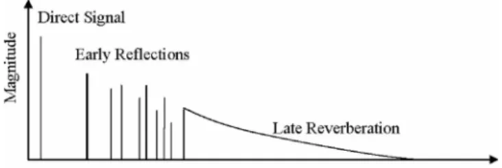
ele-ments in spatial audio reproduction. The spaciousness of repro-duced sound can be enriched by using reverberators. A room re-sponse can in general be divided into two parts, as shown in Fig. 1. The early reflection, lasting for approximately 80 ms, is com-posed of the direct sound accompanied by discrete reflections. Early reflection is dependent on room geometry as well as the relative positions of the source and the receiver. As compared to the early reflection, the late reverberation is less structural and contains extremely dense echoes with exponentially decreasing amplitude. Both parts of the response are highly complex in typi-cal diffuse sound fields and are difficult, if not impossible, to model using modal analysis.

Several statistics of the room response are relevant in the design

Fig. 2 The impulse response obtained by using the image-source method with 30th-order reflections. The room dimen-sion is 10 mà 8 m à 3 m and absorption coefficient is 0.8.

of reverberators. First, the echo density is defined in the time domain as the number of echoes per second in a room response. Kuttruff关21兴 derived the formula using a sphere model to estimate the number of echoes within time t

Nt=

4␲共ct兲3

3V 共3兲

where c is the speed of sound and V is the volume of room. Differentiating Eq.共3兲 with respect to time t gives the echo den-sity Dt= dNt dt = 4␲c3 V t 2 _共4兲

Note that echo density is proportional to the square of time. The second statistic is the modal density defined in the frequency do-main as the number of normal modes per Hertz. The number of normal modes N_f below frequency f, independent of the room geometry, can be estimated using the following formula关21兴

Nf= 4␲V c3 f 3₊␲S 4c2f 2₊ L 8cf 共5兲

where S is the area of all walls and L is the sum of all edge lengths of the room. Differentiating Eq.共11兲 with respect to time leads to the expression of modal density

Fig. 3 IIR filter structures of reverberator:_{„a… The structure of comb filter. The parameter b}pis the gain of absorbent lowpass filter and giis the gain of comb filter.„b… The structure of ten parallel comb filters and three-layer nested allpass filters._{„c… The structure of nested allpass/comb reverberator in conjunction with the} early reflection module obtained using the image method.

Fig. 4 The open-loop system including a headset, an embed-ded capacitive microphone, and a power amplifier circuit

Df= dNf df ⬇ 4␲V c3 f 2 _共6兲

Hence, the modal density of a room grows in proportion to the square of frequency. Third, the reverberation time T60is defined as

the time required for the sound pressure level to drop by 60 dB after a steady-state source is switched off. Reverberation time can be estimated by Sabine’s formula关22兴

T₆₀=0.163 · V

兺

共7兲 where V is the volume of the room; and Siand aiare the surface

area and the associated absorption coefficient. Reverberation time is proportional to the volume of the room and inversely propor-tional to the wall absorptivity and the interior surface area of the room. Because most materials become more absorptive at high

frequencies, reverberation time decreases as the frequency increases.

There are two commonly used methods for predicting the early reflection of a room: the ray-tracing method and the image-source method关23,24兴. The ray-tracing method is based on the assump-tion that sound behaves like rays in high frequencies. The distri-bution of sound field is determined by keeping track of the ray that passes each cell position in the space. On the other hand, the image-source method models the reflections from the room boundary as the sound wave emitted by virtual sources. Although image sources can be created indefinitely, only early reflections are computed in practice by utilizing low-order image sources. This method is particularly suited to the calculation of responses of regularly shaped rooms. The image method is employed in the paper to calculate the early reflections of room responses. For a rectangular room, the number of image sources required in the calculation of the nth-order reflection can be estimated as

Nn= 4n2+ 2 共8兲

The number of image sources grows with the square of n. The impulse response of the room is constructed by recording all ar-rivals of the impulses from the primary source and the image sources as well. The impulse response due to the image sources is an attenuated and delayed version of the response due to the pri-mary source. The resulting sum of impulses serves as the coeffi-cients of the FIR filter for the early reflections of the room re-sponse. Figure 2 illustrates the impulse response calculated using

Fig. 5 The measured frequency response of the plant between 100 kHz and 25.6 KHz

Fig. 6 The block diagram of the active headset system. The unity-feedback system is the QFT-based ANC module, whereas the feedforward system is the 3D spatial audio module.

Fig. 7 Nichols chart of the plant templates measured at frequencies 500, 1 kHz, 1.5 kHz, 2 kHz, 3 kHz, and 4 kHz.

the image-source method up to the 30th-order reflection. In addition to the early reflection, the late reverberation is re-quired to complete the room response. Referring to Fig. 3, the method we used for synthesizing the late reverberation is a comb filter and all-pass filter network 关25兴. The parallel comb filters serve to increase modal density and echo density, wheras series allpass filters serve to further increase echo density of reverbera-tion. The filter parameters are dependent on the modal density and echo density associated with a particular room. The feedback gains g_iof the comb filters can be chosen according to a desired reverberation time关26兴

gi= 10−3mi·Fs/T60 共9兲

The absorbent filter in Fig. 3共a兲 is a first-order low-pass filter

whose parameters are determined by the ratio␣ of the reverbera-tion times at the Nyquist frequency and dc关27兴. The gain of the absorbent filter bpis given as关26兴

bp= 1 −

2

1 + g关1−共1/␣兲兴 共10兲 The network structure comprising ten parallel comb filters and three-layer nested allpass filters is shown in Fig. 3共b兲. Figure 3共c兲 shows the complete network structure of the nested allpass/comb reverberator, combined with the early reflection designed using the image-source method. More details of the design procedure of the reverberator network can be found in Ref.关28兴.

4 ANC Design Based on the QFT

This section begins with the ANC design for the headset using the QFT technique. The design procedure is carried out with the aid of theMATLABQFTTOOLBOX关29兴. A QFT procedure typically involves three basic steps:共1兲 computation of QFT bounds; 共2兲 design of the controller; and共3兲 detailed analysis of the design.

The QFT design, performed in the frequency domain, follows very closely the classical loop-shaping designs using Bode plots. One of the design goals is to meet the performance specifications in the presence of plant uncertainties共robust performance兲. Prior to the design, plant frequency response templates with uncertainty models must be generated. For the plant templates, the QFT con-verts the closed-loop magnitude specifications into the magnitude and phase constraints, the QFT bounds, on a nominal open-loop function. A nominal open-loop function is then designed to satisfy its QFT bounds, as well as to achieve nominal closed-loop stabil-ity. The detailed procedure is given as follows.

4.1 Plant Model. One of the advantages of the QFT is that

only frequency response of the plant is needed for the design. It is generally easier to measure the frequency responses than to estab-lish an analytical transfer function model for complex systems. For the headset in Fig. 4, the plant P considered herein is defined as the system between the loudspeaker of the headset with an amplifier 共the actuator兲 and an embedded microphone 共the sen-sor兲. Several frequency responses of the open-loop plant are mea-sured. Here, in Fig. 5, one of the frequency responses from 100 Hz to 25.6 kHz, measured by properly wearing the headset, is taken as the nominal plant. On the other hand, the difference between the other wearing scenarios 共including improper ways兲 and the nominal plant is considered as uncertainty. For this plant, a unity-feedback controller along with a feedforward controller is employed as the control structure for our problem, as shown in Fig. 6.

4.2 Design Specifications. The first specification to be met in

the control design is robust stability. We seek to design a control-ler G共s兲 such that the closed-loop transfer function, or the comple-mentary sensitivity function, satisfies

冏

1 + P共j␻兲G共j␻兲

冏

lower gain margin = 1 + Ws−1

lower phase margin = 180 deg −␪,␪ = cos−1_共0.5W

s

−1_{− 1兲}

苸 关0,180 deg兴 where W_Sis a constraint bound index.

We place more emphasis on performance requirement on noise

Fig. 8 QFT bounds at several frequencies, indicated with dif-ferent colors. The frequencies are indicated in the legend at the top left corner.„a… Robust margin bounds at frequencies 500,

1 kHz, 1.5 kHz, 2 kHz, 3 kHz, 4 kHz.„b… Robust output

distur-bance rejection bounds at frequencies 500, 1 kHz, 1.5 kHz._„c… Robust spillover rejection bounds at frequencies 2 kHz, 3 kHz, 4 kHz.

reduction by using a high-pass weighting filter described by Eq. 共12兲, with the bandwidth ranging from 500 Hz to 2 kHz. We wish to achieve 10 dB reduction by this design. The specification is

robust output disturbance rejection, described by the sensitivity function关30,31兴. In the paper, a high-pass filter is chosen as the constraint bound

冏

冏

冏

冏

冏

冏

However, spillover will also arise in the band 2 – 5 kHz due to the performance requirement by Eq.共12兲. Thus, the controller is

designed to ensure the spillover does not exceed 4.6 dB in the band from 2 kHz to 5 kHz. Hence, the third control specification

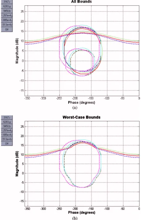
Fig. 9 QFT loop-shaping on the Nichols chart:_{„a… superposition of all bounds;}

is spillover rejection, which constrains spillover at a specified fre-quency band. The specification of spillover rejection chosen for our problem is

Spillover rejection艋 1.7共4.6 dB兲,␻ 苸 共2000,5000兴 Hz 共13兲

4.3 Plant Templates. The term plant template refers to the

collection of measured frequency responses at a given frequency of the system subject to uncertainties. In the QFT design, we have to select a frequency array for computing plant templates and bounds as explained below. In considering the design bandwidth of our case, frequency array 500, 1 kHz, 1.5 kHz, 2 kHz, 3 kHz, 4 kHz are chosen. The plant templates at frequency array are shown in the Nichols chart of Fig. 7 along with their boundary. One of these templates is designated as the nominal plant in the subsequent QFT design.

4.4 Working With Bounds. Using the plant templates, the

QFT converts closed-loop magnitude specifications into magni-tude and phase constraints, or the QFT bounds, on a nominal open-loop function in the Nichols chart. The Nichols chart dis-plays complex frequency response functions in terms of their magnitude共in dB兲 and phase 共in degrees兲. A nominal open-loop function 共GP兲 is then designed to satisfy these bounds and to

achieve robust stability. The margin bounds at frequencies 500, 1 kHz, 1.5 kHz, 2 kHz, 3 kHz, 4 kHz are shown in Fig. 8共a兲. Next QFT design focuses on the robust performance of the closed-loop system in the band 500– 2000 Hz. The robust output sensi-tivity bounds at frequencies 500, 1 kHz, 1.5 kHz are shown in Fig. 8共b兲. Finally, the bounds for the robust spillover rejection are shown in Fig. 8共c兲 for several frequencies within the desired per-formance bandwidth关2000,5000兴 Hz. Superposition of all bounds is shown in Fig. 9共a兲. In general, when the problem involves more than one set of bounds, one should compute the worst-case bound as shown Fig. 9共b兲 of all sets, i.e., the intersection of all bounds, which is easier to work with than with a collection of bounds.

4.5 Loop Shaping and Analysis. Having computed the

sta-bility and performance bounds, the next step in a QFT design involves the loop shaping of a nominal open-loop function共GP兲 that meets the previously found bounds. The QFT design provides such an interactive environment for loop shaping in the Nichols chart. The nominal open-loop response and the associated bounds are drawn in Fig. 10共a兲. We are seeking to design a nominal loop function L₀共s兲= P₀共s兲G共s兲, where P₀共s兲 is the nominal plant, that shall attain the aforementioned specifications. In words, loop

Fig. 10 Nichols chart of the open-loop response G„s…P„s…: „a…

uncompensated open-loop response and its bounds; and„b…

compensated open-loop response with a sixth-order controller

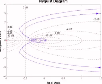
Fig. 11 Nyquist diagram of the open-loop system G„s…P„s…

Fig. 12 The sensitivity function„dashed line… and the

shaping involves adding poles and zeros until the nominal loop lies near its bounds and results in nominal closed-loop stability. The QFT procedure enables the users to consider different con-troller complexities and weigh possible tradeoffs. The concon-troller G共s兲 is designed by adding poles and zeros in the Nichols chart to satisfy the aforementioned specifications. The result after loop shaping is shown in Fig. 10共b兲.

In the present design, robust stability has been achieved since the nominal loop does not violate the robust margin bounds and does not cross the ray关32兴

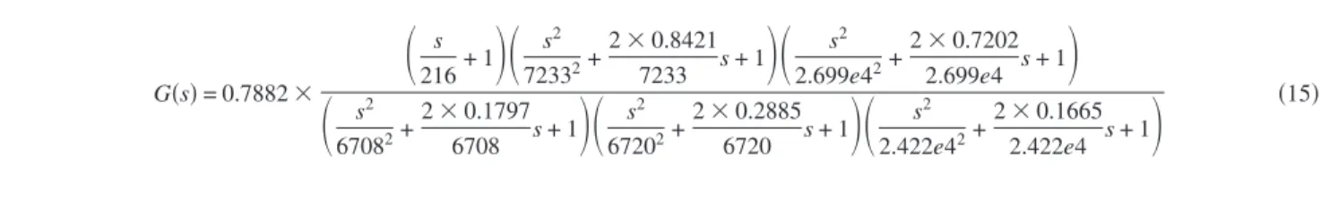
R =兵共␾,␥兲: ␾ = −180 deg, ␥⬎0 dB其 共14兲 The feedback controller resulted from the interactive QFT de-signed is given by the following sixth-order transfer function

G共s兲 = 0.7882 ⫻

冉

冊冉

冊冉

冊

冉

冊冉

冊冉

冊

For the design, it is advisable to check if the close-loop system is stable by using the Nyquist plot as shown in Fig. 11. It is con-cluded that the closed-loop system is stable because the frequency response curve does not encircle the critical point共−1,0兲.

The sensitivity function共the dotted line兲 and the complemen-tary sensitivity function共solid line兲 pertinent to the present design are shown in Fig. 12. The results reveal that the performance is attained within 700– 2 kHz, and the spillover rejection is also sat-isfied within 2 K – 5 kHz.

5 Experimental Verification

5.1 ANC Performance. Hardware was implemented to

inte-grate the above-mentioned 3D spatial audio and ANC into a single

unit. First, the QFT-based active feedback controller is realized by using analog circuits because, after preliminary evaluation, we found that the delay of the DSP is much too large to afford a digital design. The analog circuits of the sixth-order controller as designed previously can be easily implemented using operational amplifiers 共OPs兲, following the design method of active biquad filters关33兴. The resulting circuit of the feedback controller G共s兲 is shown in Fig. 13. Figure 14 shows the implemented frequency response of the QFT controller 共solid line兲 that compares quite well in the control bandwidth to the designed response 共dotted line兲.

To assess the performance of the ANC, the headset was worn by an acoustic manikin. A 2 in. condenser microphone was

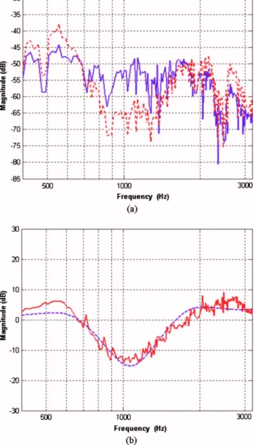
mented in the ear canal of the manikin. A 3.5 in. full range loud-speaker positioned 1 m away from the manikin, playing white noise, served as the extraneous noise source. The test was con-ducted inside an anechoic chamber. The sound pressure responses measured by the microphone with and without active control are compared in Fig. 15共a兲. Noise attenuation was achieved in the band 700– 1700 Hz. The maximal attenuation reached 13 dB in the band. These results compare quite well with those predicted by the sensitivity functions shown in Fig. 15共b兲.

5.2 Subjective Listening Test of the Integrated System. A

listening test was carried out to examine the total system that integrated the 3D spatial audio and the ANC. A feedforward mod-ule that implements the 3D audio effects was realized by using a fixed-point DSP, ADI BF-533. The 3D audio effects considered herein are the aforementioned HRTF and the reverberator. The feedforward 3D audio module was connected to the previously mentioned analog feedback ANC module to form a hybrid control system共Fig. 6兲. To assess the proposed system, subjective listen-ing experiments were conducted. Six subjective indices includlisten-ing sound image definition, spaciousness, ambience, clarity, natural-ness, and externalization are selected for the listening tests. Ten subjects took part in the test. Listeners’ perception in terms of the subjective indices was answered in a questionnaire on a scale ranging from −5 to 5. The 3D audio presentation without ANC was taken as the benchmark. The grade 0 indicates “no differ-ence” between the audio presentation under test and the uncon-trolled benchmark. A grade greater/less than zero indicates that the controlled/uncontrolled signal perceptually outperforms the uncontrolled/controlled signal, in terms of a particular subjective index. Figure 16 illustrates the result of the subjective listening test in which the average grades for each index are summarized. It is evident from the result that the 3D audio-ANC headset per-formed well in all indices共with all positive grades兲, as compared to the headset with no ANC. As anticipated, the grade of clarity was not as high as the other indices since the reverberator in the 3D module would adversely affect this particular aspect. To fur-ther assess the significance of the result, an ANOVA test was conducted. Table 1 shows the result of the ANOVA test. It is interesting to note that the significance value of clarity is above the commonly chosen threshold of 0.05, indicating the grade in this aspect was somewhat disputed. But, overall, the difference made by the new system is statistically significant, as revealed by the fact that the significance values shown in Table 1 are mostly well below the threshold of 0.05. It is then concluded from the

Fig. 14 Frequency response functions of the feedback con-troller:„solid line… designed; „dashed line… implemented

Fig. 15 Results of the active noise cancellation: „a… sound

pressure spectra measured by the microphone with _„dashed line… and without „solid line… the active control; and „b…

sensi-tivity function; _{„solid line… measurement; „dashed line…} simulation

Fig. 16 The average grades of subjective indices obtained from the listening test

results that the ANC proved to be useful in enhancing 3D spatial sound reproduction by using a headset.

6 Conclusions

A headset that integrates the QFT-based ANC and 3D spatial audio processing technologies has been proposed in the paper. It is demonstrated that active control approaches can be used to en-hance the performance of 3D audio. As pointed out by the re-viewer, some examples of active control from the recent JVA publications are also along this line关34,35兴. The active noise can-celler was designed by using the QFT loop-shaping technique which yielded a feedback controller with various control perfor-mance and robustness specifications taken into account. The low-order controller was implemented by using analog circuits to minimize the loop delay. Noise attenuation was achieved in the band 700– 1700 Hz. The maximal attenuation reached 13 dB in the band.

The feedback ANC and the feedforward 3D audio are then in-tegrated into the headset. It is observed from the result that the combined system performed well in all indices, as compared to the headset with no ANC. In addition, the difference made by the combined system is statistically significant, as revealed by the fact that the significance values shown in the AVOVA test are mostly well below the threshold of 0.05. It is then concluded from the results that the ANC proved to be useful in enhancing 3D spatial sound reproduction by using a headset.

Acknowledgment

The work was supported by the National Science Council 共NSC兲 in Taiwan, under Project No. NSC 92-2212-E009-030. References

关1兴 Horowitz, I. M., 1963, Synthesis of Feedback Systems, Academic, New York. 关2兴 Horowitz, I. M., and Sidi, M., 1972, “Synthesis of Feedback Systems With Large Plant Ignorance for Prescribed Time-Domain Tolerances,” Int. J. Con-trol, 16共2兲, pp. 287–309.

关3兴 Horowitz, I. M., 1992, Quantitative Feedback Theory (QFT), QFT Publica-tions, Boulder, CO.

关4兴 Gardner, B., and Martin, K., 1994, “HRTF Measurements of KEMAR Dummy-Head Microphone,” MIT Media Lab, http://sound.media.mit.edu/ KEMAR.html

关5兴 Batteau, D. W., 1967, “The Role of the Pinna in Human Localization,” Proc. R. Soc. London, Ser. B, 168, pp. 158–180.

关6兴 Batteau, D. W., 1968, Listening with the Naked Ear: The Neuropsychology of

Spatially Oriented Behavior, Dorsey Press, Homewood, IL.

关7兴 Wright, D., Hebrank, J. H., and Wilson, B., 1974, “Pinna Reflections as Cues for Localization,” J. Acoust. Soc. Am., 56共3兲, pp. 957–962.

关8兴 Algazi, V. R., Duda, R. O., Thompson, D. M., and Avendano, C., 2001, “The CIPIC HRTF Database,” Proceedings IEEE Workshop on Applications of

Sig-nal Processing to Audio and Electroacoustics, Avignon, August 1988, Mohonk

Mountain House, New Paltz, NY, pp. 99–102, http:// interface.cipic.ucdavis.edu/

关9兴 Lueg, P., 1936, “Process of Silencing Sound Oscillations,” US Patent No. 2,043,416.

关10兴 Bai, M., and Lee, D., 1997, “Implementation of an Active Headset by Using the H_⬁Robust Control Theory,” J. Acoust. Soc. Am., 102共4兲, pp. 2184–2190. 关11兴 Elliott, S. J., Stothers, I. M., Nelson, P. A., McDonald, A. M., Quinn, D. C., and Saunders, T., 1988, “The Active Control of Engine Noise Inside Cars,”

Proceedings Inter-noise, San Diego, CA, pp. 987–990.

关12兴 Dorling, C. M., Eatwell, G. P., Hutchins, S. M., Ross, C. F., and Sutcliffe, S. G. C., 1989, “A Demonstration of Active Noise Reduction in an Aircraft Cabin,” J. Sound Vib., 128共2兲, pp. 358–360.

关13兴 Elliott, S. J., and Nelson, P. A., 1994, “Active Noise Control,” Noise News Int., 2, pp. 75–98.

关14兴 Tohki, M. O., and Leitch, R. R., 1992, Active Noise Control, Clarendon, Ox-ford, UK.

关15兴 Fuller, C. R., and von Flotow, A. H., 1995, “Active Control of Sound and Vibration,” IEEE Control Syst. Mag., 15共6兲, pp. 9–19.

关16兴 Nelson, P. A., and Elliott, S. J., 1992, Active Control of Sound, Academic, New York, NY.

关17兴 Elliott, S. J., 2001, Signal Processing for Active Control, Academic, New York, NY.

关18兴 Olson, H. F., and May, E. G., 1953, “Electronic Sound Absorber,” J. Acoust. Soc. Am., 25, pp. 1130–1136.

关19兴 Wheeler, P. D., 1986, “Voice Communication in the Cockpit Noise Environment—The Role of Active Noise Reduction,” Ph.D. thesis, University of Southampton, Southampton, UK.

关20兴 Gay, S. L., and Benesty, J., 2000, Acoustic Signal Processing for

Telecommu-nication, Kluwer Academic, Boston, MA.

关21兴 Kuttruff, H., 1991, Room Acoustics, Elsevier, New York, NY.

关22兴 Sabine, W. C., 1972, “Reverberation,” Acoustics: Historical and Philosophical

Development, R. B. Lindsay, ed., Dowden, Hutchinson, and Ross,

Strouds-burg, PA.

关23兴 Savioja, L., 1999, “Modeling Techniques for Virtual Acoustics,” Doctorate thesis, Helsinki University of Technology, Espoo, Finland.

关24兴 Lehnert, H., and Blauert, J., 1992, “Principles of Binaural Room Simulation,” Appl. Acoust., 36, pp. 259–291.

关25兴 Gardner, W. G., 1992, “The Virtual Acoustic Room,” Master’s thesis, MIT Media Lab, Cambridge, MA.

关26兴 Frenette, J., 2000, “Reducing Artificial Reverberation Requirements Using Time-Variant Feedback Delay Networks,” Master Research Project, University of Miami, Miami, FL.

关27兴 Beltra’n, F. A., and Beltra’n, J. R., 2002, “Implementing Reverberation Algo-rithms in Matlab,” J. New Music Res., 31, pp. 153–161.

关28兴 Bai, M. R., and Bai, G., 2007, “Optimal Design and Synthesis of Reverbera-tors with a Fuzzy User Interface for Spatial Audio,” J. Audio Eng. Soc., in press.

关29兴 Borghesani, C., Chait, Y., and Yaniv, O., 2003, the QFT Frequency Domain

Control Design Toolbox User’s Guide, Terasoft, US.

关30兴 Chait, Y., and Yaniv, O., 1993, “Multi-Input/Single-Output Computer Aided Control Design Using the Quantitative Feedback Theory,” Int. J. Robust Non-linear Control, 3, pp. 47–54.

关31兴 Chait, Y., Borghesani, C., and Zheng, Y., 1995, “Single-Loop QFT Design for Robust Performance in the Presence of Non-Parametric Uncertainties,” J. Dyn. Syst., Meas., Control, 117, pp. 420–424.

关32兴 Cohen, N., Chait, Y., Yaniv, O., and Borghesani, C., 1994, “Stability Analysis Using Nichols Charts,” Int. J. Robust Nonlinear Control, 4, pp. 3–20. 关33兴 Chen, W. K., 1986, Passive and Active Filters: Theory and Implementations,

Wiley, New York, NY.

关34兴 Yuan, J., 2006, “Active Resonators for Noise Absorption,” ASME J. Vibr. Acoust., 128共1兲, pp. 115–121.

关35兴 Bisnette, J. B., Smith, A. K., Vipperman, J. S., and Budny, D. D., “Active Noise Control Using Phase-Compensated, Damped Resonant Filters,” ASME J. Vibr. Acoust., 128共2兲, pp. 148–155.

Table 1 Significant values of the ANOVA test on the listening experiment

Subjective index Significance value

Sound image definition 9.8834e − 6

Spaciousness 4.1488e − 6

Ambience 4.1488e − 6

Clarity 1.4111e − 1

Naturalness _{1.5280e − 3}