利用對稱式樹狀預測架構在AVC中有效實現視訊正轉、倒轉、快轉及隨機擷取

國

立

交

通

大

學

電子工程學系電子研究所碩士班

碩

士

論

文

利用對稱式樹狀預測架構在 AVC 中有效實現視訊

正轉、倒轉、快轉及隨機擷取

Efficient VCR Functionality Implementation in

AVC with Symmetric Tree Prediction Structure

指導教授：蔣迪豪 博士

研 究 生：楊思浩

利用對稱式樹狀預測架構在 AVC 中有效實現視訊正轉、倒轉、

快轉及隨機擷取

Efficient VCR Functionality Implementation in AVC with

Symmetric Tree Prediction Structure

研 究 生: 楊思浩

S t u d e n t: S.H. Yang

指導教授: 蔣迪豪

A d v i s o r: Tihao Chiang

國 立 交 通 大 學

電子工程學系電子研究所碩士班

碩 士 論 文

A Thesis

Submitted to Department of Electronics Engineering & Institute of Electronics College of Electrical Engineering and Computer Science

National Chiao Tung University in partial Fulfillment of the Requirements

for the Degree of Master

in

Electronics Engineering

July 2005

HsinChu, Taiwan, Republic of China

利用對稱式樹狀預測架構在 AVC 中有效實現視訊正轉、倒

轉、快轉及隨機擷取

研究生: 楊思浩

指導教授: 蔣迪豪 博士

國立交通大學

電子工程學系 電子研究所碩士班

摘要

我們提出了一種新的時間軸預測架構，將一串影像對稱式的拆解為

數個階層。這種架構提供了所有的 VCR 功能如:隨機存取，快速正/倒

轉。我們將這種階層式的架構命名為對稱式樹狀預測架構。我們利用

AVC 提供的影像參照處理機制來設定並壓縮出符合 AVC 標準的對稱式

樹狀預測架構二位元資料串流。對稱式樹狀預測架構在解壓縮端提供

了極有效率的快速 正/倒 轉，在快轉時，不需播放的影片可以略過不

解壓縮。對稱式樹狀預測架構只須壓縮一次，就可以單一的二位元資

料串流在解壓縮端提供所有的 VCR 功能。 我們提供了相當有彈性的參

數設定，使我們可以任意變更其樹狀架構，使其有較好的壓縮效能或

是提供較低複雜度的壓縮。最後的實驗結果顯示，對稱式樹狀預測架

構其壓縮效能和一般壓縮方式相當接近，雖花了稍高的複雜度，但在

解壓縮端可以提供極低複雜度的 VCR 實現。

Tree Encoder with Long Term Prediction

Fast Forward and Inverse Playback in Decoder

Student: Su hao Yang

Advisor: Dr. Tihao Chiang

Institute of Electronics

National Chiao Tung University

Abstract

We present a novel technique, hierarchical temporal domain decimated prediction structure, to provide a video bitstream with full VCR functionality – random access, fast forward, and fast backward. This hierarchical temporal domain decimated prediction structure, which we named as symmetric tree prediction structure, utilized the flexible reference picture management scheme that provided in AVC standard to generate an AVC compliant bitstream. It uses a tree-like prediction structure to provide efficient fast forward/fast backward playback functionality. No redundant picture will be decoded during fast playback. Only one-pass encoding and a single bitstream can provide both the forward and backward playback functionality. It also provides flexible parameters to make the prediction structure can be tuned with better coding efficiency or lower complexity. We also propose a decoder that can fully support the VCR functionality with low complexity. The simulation results show the symmetric tree prediction structure can provide full VCR functionality with similar coding efficiency and slightly higher coding complexity.

誌謝

在碩士生涯當中，我學會研究生必備的＂做研究的方法＂，不但要學習並了 解前人的知識，參考前人的實驗及想法，最重要的還要具有自我思考能力，方能 找出新東西的蛛絲馬跡。這些事情聽起來簡單，但是這個過程確是每個碩士生從＂ 學生＂轉到＂研究生＂最艱難但是最必要的一步了。要走出這一步最重要及最要 感謝的就是教授和學長了，想想在剛踏入研究生之初，每每為了如何找出一條前 人未走的道路而不斷的苦惱及思索著，此時蔣迪豪教授和黃項群學長每每都能幫 我點亮一道道明燈，從一開始的分析過去的演算法，推敲新的演算法，並思考著 實用性及實現的可能性，因為研究就像下棋一般，一子錯則滿盤皆墨，不是走一 步算一步，全盤的思考是相當必要的，和大學時代只要學會書上的知識來應付考 試大不相同的。在教授和學長的引領之下，使我在崎嶇難行的研究路上還能走得 順風順水，如御風而行。 在研究生的日子中，研究室戰友們也是我不可或缺的重要資源了。如果指導 教授和學長是空氣的話，研究室戰友們就是水和糧食了。這些戰友是千金難買的， 在研究上，學長們如莊孝強，蘇子良，大范，和 Vision LAB，漢光 我們一同研究， 討論我們的實驗，討論 spec，討論 sequence 及作業，在玩樂時 Vision LAB, A LAB, Wireless LAB，我們一致對外，一同爭取 NCTUEE 的勝利。這些實驗室的戰友，使 我從大學的孤軍作戰到現在 team work 好手，大家在苦難中一同成長，在玩樂中 一同歡笑，謝謝大家這二年來的相互扶持。

還要感謝的就是蔣老師研室群的同學們及學長學弟，osban 和世騫陪我一同 走過由戰戰競競到歡樂無邊的 group meeting。在 group meeting 中，文孝學長的 完美演出，項群學長的 spec 功力，士豪學長的實事求是，志鴻學長的盡善盡美， 另外學弟們也各各都是臥虎藏龍，genius 人如其名，阿旦文武雙全，新任班長則 成績優良，事事爭先，韋霖學弟則常常通宵達旦研究到天明，很高興加入這個實 驗室。 最後，家人的支持是我不斷努力下去的原動力，交大這六年一路走來， 作業和考試也曾經考到我怕過，研究之路也曾經讓我迷惘過是否我有能力讀研究 所，還是我只是想偽裝知識分子混個文憑來找工作，但是在家人和同儕的相護提 攜之下，我了解了努力讀書研究的目的，並順利的畢業了，成功完成了我在學業 上的目標。

Index

CHAPTER 1 INTRODUCTION ...1 1.1 MOTIVATION...1 1.2 APPLICATION SCENARIO...3 1.3 ORGANIZATION...4 CHAPTER 2 BACKGROUND...5 2.1 PREVIOUS WORK...5

2.2 ADVANCED VIDEO CODING...9

2.2.1 Overview...9

2.2.2 Reference picture management process... 11

CHAPTER 3 TREE ARCHITECTURE CODER ...20

3.1 BASIC CONCEPT OF OUR TREE PREDICTION STRUCTURE...20

3.2 SYMMETRIC TREE STRUCTURE ENCODER IMPLEMENTATION IN AVC...25

3.3 DECODER IMPLEMENTATION THAT SUPPORT VCR FUNCTIONALITIES...31

3.4 COST OF VCRFUNCTIONALITIES FOR VARIOUS GOPSTRUCTURES...35

3.4.1 Cost of forward and backward playback for normal GOP structure...35

3.4.2 Cost of forward and backward playback for symmetric tree prediction structure with different level depth ...42

3.4.3 The Comparison of P and B picture in Symmetric Tree Prediction Structure ...49

3.4.4 Decoding complexity for fast playback and random access ...52

CHAPTER 4 EXPERIMENTAL RESULTS ...55

4.1 CODING EFFICIENCY COMPARISON FOR DIFFERENT LEVEL DEPTHS...56

4.2 CODING EFFICIENCY COMPARISON FOR DIFFERENT P/B LEVEL DEPTHS...59

4.3 CODING EFFICIENCY COMPARISON FOR DIFFERENT REFERENCE PICTURE NUMBER 62 4.4 CODING EFFICIENCY COMPARISON WITH NORMAL GOP STRUCTURE...66

CHAPTER 5 CONCLUSION...70

L

IST OF

F

IGURES

FIGURE 1-1 UTILIZED THE PROPOSED SYMMETRIC TREE PREDICTION STRUCTURE TO SERVE

VIDEO PLAYBACK WITH VCR FUNCTIONALITIES. ...3

FIGURE 2-1 BINARY TREE STRUCTURE WITH N=15[1] ...8

FIGURE 2-2 PROPOSED GOP STRUCTURE OF PREVIOUS WORK[1] ...8

FIGURE 2-3AVC ENCODER [2]...10

FIGURE 3-1 INTRA FRAME ENCODING...23

FIGURE 3-2IPPP ENCODING...23

FIGURE 3-3 BEST RANDOM ACCESS FOR INTER PREDICTION...23

FIGURE 3-4PREDICTION METHOD FOR THE NEAREST LEVEL...24

FIGURE 3-5AN EXAMPLE OF A PGOP WITH VARIOUS DESCENDENT PICTURE NUMBER AND DEPTH.EACH CIRCLE INDICATES A PICTURE.THE BLACK CIRCLE IS THE ROOT I-PICTURE.THE RED CIRCLES ARE THE PIDR-PICTURES.THE GREEN CIRCLES ARE THE LEAF PICTURES...24

FIGURE 3-6SYMMETRIC TREE PREDICTION STRUCTURE FOR N16_P1_B1_B3...27

FIGURE 3-7CODING ORDER FOR GOP STRUCTURE N16_P1_B1_B3 ...28

FIGURE 3-8 LONG TERM PICTURE NUMBERS SETTING FOR GOP STRUCTURE N16_P1_B1_B3 ...28

FIGURE 3-9GET PTS AND SBP OF ALL 1ST FRAME OF EACH GOP...33

FIGURE 3-10 DECODER FLOW CHART...34

FIGURE 3-11 FORWARD PLAYBACK FOR IPPPGOP STRUCTURE...37

FIGURE 3-12 INVERSE PLAYBACK FOR IPPPGOP STRUCTURE...38

FIGURE 3-13IPBGOP STRUCTURE...39

FIGURE 3-14 FORWARD PLAYBACK FOR IPBGOP STRUCTURE...40

FIGURE 3-15 REVERSE PLAYBACK FOR IPBGOP STRUCTURE...41

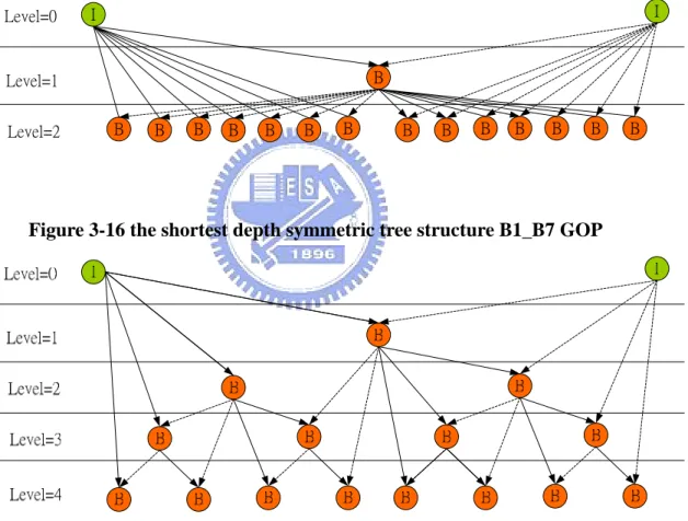
FIGURE 3-16 THE SHORTEST DEPTH SYMMETRIC TREE STRUCTURE B1_B7GOP...44

FIGURE 3-17 THE LONGEST DEPTH OF SYMMETRIC TREE STRUCTURE 4B1GOP...44

FIGURE 3-18 FORWARD PLAYBACK DECODING DIAGRAM OF B1_B7GOP STRUCTURE...45

FIGURE 3-19 INVERSE PLAYBACK DECODING DIAGRAM OF B1_B7GOP STRUCTURE...46

FIGURE 3-20 FORWARD PLAYBACK DECODING DIAGRAM OF 4B1GOP STRUCTURE...47

FIGURE 3-21 INVERSE PLAYBACK DECODING DIAGRAM OF 4B1GOP STRUCTURE...48

FIGURE 3-22P1_3B1GOP STRUCTURE...51

FIGURE 4-1RD-CURVES OF BUS SEQUENCES FOR TREE STRUCTURE WITH VARIOUS LEVEL DEPTHS...57

FIGURE 4-2RD-CURVES OF FOREMAN SEQUENCES FOR TREE STRUCTURE WITH VARIOUS LEVEL DEPTHS...57

FIGURE 4-3RD-CURVES OF MOBILE SEQUENCES FOR TREE STRUCTURE WITH VARIOUS LEVEL DEPTHS...58 FIGURE 4-4RD-CURVES OF FOOTBALL SEQUENCES FOR TREE STRUCTURE WITH VARIOUS

LEVEL DEPTHS...58 FIGURE 4-5RD CURVE OF BUS SEQUENCE WITH DIFFERENT P/B IN EACH LEVEL...60 FIGURE 4-6RD CURVE OF FOREMAN SEQUENCE WITH DIFFERENT P/B IN EACH LEVEL....60 FIGURE 4-7RD CURVE OF MOBILE SEQUENCE WITH DIFFERENT P/B IN EACH LEVEL...61 FIGURE 4-8RD CURVE OF FOOTBALL SEQUENCE WITH DIFFERENT P/B IN EACH LEVEL...61 FIGURE 4-9 THE RD CURVE OF BUS WITH DIFFERENT NUMBERS OF REFERENCES...63 FIGURE 4-10 THE RD CURVE OF FOREMAN WITH DIFFERENT NUMBERS OF REFERENCES..64 FIGURE 4-11 THE RD CURVE OF MOBILE WITH DIFFERENT NUMBERS OF REFERENCES...64 FIGURE 4-12 THE RD CURVE OF FOOTBALL WITH DIFFERENT NUMBERS OF REFERENCES.65 FIGURE 4-13RD CURVE OF BUS SEQUENCE WITH NORMAL AND SYMMETRIC TREE

STRUCTURE COMPARISON...68 FIGURE 4-14RD CURVE OF FOREMAN SEQUENCE WITH NORMAL AND SYMMETRIC TREE

STRUCTURE COMPARISON...68 FIGURE 4-15RD CURVE OF MOBILE SEQUENCE WITH NORMAL AND SYMMETRIC TREE

STRUCTURE COMPARISON...69 FIGURE 4-16RD CURVE OF FOOTBALL SEQUENCE WITH NORMAL AND SYMMETRIC TREE

List of Tables

TABLE 3-1 REFERENCE PICTURE LIST OF EACH PICTURE OF GOP STRUCTURE

N16_P1_B1_B3 ...29 TABLE 3-2 MAXIMUM ENCODER BUFFER SIZE AND DECODING DELAY IN DIFFERENT P/B

DEPTH...51

TABLE 3-3SYMMETRIC TREE STRUCTURE FAST FORWARD PLAYBACK TRANSMISSION TABLE...53

TABLE 3-4SYMMETRIC TREE STRUCTURE FAST INVERSE PLAYBACK TRANSMISSION TABLE

...53 TABLE 3-5 NORMAL GOP STRUCTURE WITH IPPP FAST FORWARD PLAY BACK

TRANSMISSION TABLE...53

TABLE 3-6 NORMAL IPPPGOP STRUCTURE WITH UNLIMITED BUFFER SIZE FAST INVERSE PLAYBACK TRANSMISSION TABLE...53

TABLE 3-7:RANDOM ACCESS DECODING DELAY OF EACH PICTURE FOR VARIOUS GOP STRUCTURES...54

TABLE 4-1 MAX AND AVERAGE DELAY COMPARISON WITH NORMAL STRUCTURE AND

Chapter 1

Introduction

1.1 Motivation

In the age of video tape, the video is record in the video tape without compression. All the VCR functionalities including step forward, step backward, fast forward, fast backward and random access can be easily supported. However, it is not the case for digital video. To reduce the storage space or transmission bandwidth, digital video is usually compressed before store or transmission. Temporal prediction is an essential tool for digital video compression. In the encoding process, previous reconstructed frame is used to predict the current frame; only the prediction error will be store. The current reconstructed frame is also used to predict the following frame. This prediction strategy removes the temporal redundancy among frames, but also causes temporal dependency. To reconstruct the current frame, the decoder must decode the previous frame to generate correct prediction image. And to decode the previous frame the decoder need to decode the frame before the previous frame – the current frame is depend on the entire previous frames. Temporal dependency won’t cause any disadvantage in a forward- only playback scenario. However, forward-only playback is not sufficient for real-word applications. The user may randomly jump to other sections in the video, fast forward playback to skip some video, or rewind the video. All of this functionality is hard to implement under the traditional temporal prediction scheme.

To address the random access issue, the traditional approaches periodically insert the intra-prediction-only picture to break the temporal dependency with other images.

However, without removing the temporal dependency, the I-picture usually needs much more bit to provide similar video quality compare with the pictures has utilized temporal predictions. To provide the fast forward functionality, the decoder can simply skip the B-picture in the bitstream. For example, with the GOP structure like …PBBBP…, the decoder can skip one B-picture for 2x forward playback speed, or skip all B-picture for 4x forward playback speed. However, if there is no B-picture in the bitstream, or more forward speed factor is needed, the decoder needs to decode some “redundant” P-pictures that are never displayed. This may waste the decoding power, or also limit the speed up factor of the decoder. To provide the (fast) backward functionality, generally there are two approaches. The first approach is, the decoder can buffer the entire already decoded picture in a GOP, and display the target image when they request. The second approach is, the decoder decode the bitstream several times. Each times it starts from the I-picture of this GOP to the target picture. Assuming there are N-picture in a GOP, the first approach need at most N-picture buffer to store all the decoded image, and the second approach need at most NxN/2 times decoding power, both are significantly need to be improved.

H.264/AVC, the latest international video-coding standard, provides a significantly improved video coding efficiency compared with the previous international standard, such as MPEG-2 and MPEG-4. It uses the variable block size motion estimation, context-based entropy coding, rate-distortion optimized, in-loop deblocking filter, and some other technique to improve the coding efficiency. It also provide a flexible reference picture management and utilization scheme to support temporal prediction. It uses multiple reference picture motion compensation, decouples the reference order from the display order, and also decouples the picture representation from the picture referencing capability [7]. In this thesis, we utilize this flexible temporal prediction structure to construct a “symmetric tree prediction structure”, which

can provide an AVC compliant video bitstream that fully support the VCR functionalities.

1.2 Application

Scenario

Figure 1-1 shows the application scenario that utilized the proposed symmetric tree prediction structure to serve video playback with VCR functionalities. The encoder encodes the video sequences with the selected symmetric tree prediction structure that suitable for the application. The bitstream is stored in the bitstream container, which could be a CD, a file in the PC, or the video server in Internet. The user or client will access the bitstream through our proposed decoder that supports VCR functionalities. Various request, including forward playback, backward playback, fast playback, and also random access, will be send to the proposed decoder, the decoder decode the requested frame and send it to the user or client.

video playback with VCR functionalities.

1.3 Organization

The details of the proposed symmetric tree prediction structure encoder and the proposed VCR-functionality-supported decoder will be described in the following chapters. The organization and abstract of each chapter are described as follows:

In Chapter 2, some previous works that address VCR functionality for video compression will be introduced first. An overview of Advanced Video Coding (AVC) will be given then. Some highlight features in AVC are briefly described. The reference picture management and utilization method in AVC, which is strongly related with the proposed structure, will be described in detail.

In Chapter 3, we firstly describe the basic concept of the proposed symmetric tree prediction structure. Then the implementation detail in AVC of the proposed structure is described. Further, we describe the concept of the proposed decoder that support VCR functionality. The decoder flow is described step by step. Finally, we discuss the cost of VCR functionality for normal GOP structure as well as the proposed structure. The trade-off among various symmetric tree prediction structures are discussed in detail.

In Chapter 4 we show the experimental results. The coding efficiency of various symmetric tree prediction structures is compared. We also compare the coding efficiency between the proposed structure and the normal GOP structures.

The conclusions are given in Chapter 5. We highlight the properties of the proposed prediction structure and the decoder that support VCR functionality.

Chapter 2

Background

2.1 Previous

Work

The normal video encoding uses sequential temporal prediction so the reference dependency is the same as the picture coding order of the GOP. If the GOP size is large, the dependencies of later frames cause serious problem for achieving VCR functionality.

In previous works, there are some techniques to implement VCR functionalities. In [1], macroblock-based scheme is proposed to use the reverse play operation. It divides all the macroblocks to forward macroblocks (FMB) and backward macroblocks (BMB). They define MBn(k,l) which means that the macroblock is the nth frame and at kth row and lth column. MBn-1(k,l) is defined as BMB if MBn (k,l) has the same spatial position, for example, MBn (k,l) is coded without motion compensation. Otherwise, it is defined as FMB. In backward display, FMB is reconstructed by the formula:

MBn (k,l) = MC MBn-1 (mvn(k,l))+en(k,l)

MC MBn-1 is the motion compensated macroblock of MBn (k,l). en is the prediction error.

BMB is reconstructed by the formula: (due to MC MBn-1 (mvn(k,l)) = 0) MBn (k,l) = MBn-1 (k,l)+en(k,l)

Ö MBn-1

(k,l) = MBn (k,l) - en(k,l).

In the algorithm, if we want to play frame n-1 after play frame n, BMB can be display with parsing en(k,l), but FMB is in the different situation. All related

macroblocks in frame n-2 which are the motion compensated macroblocks of FMB in frame n-1 needs to be sent. The BMB is the saving part in the algorithm. But the percentage of BMB is different by sequence and it just use for step reverse playback. If we want fast forward / reverse playback, the percentage of BMB will be little. The improvement for full VCR functionalities is limited.

In [2], another previous work uses video transcoding for fast forward / backward video playback. It must define different GOP structure for different speed display. If the required frame is the first frame of the GOP, it is set as intra frame. Otherwise it is set as inter frame. For example, the original sequence is 0th to 17th frame with 0th and 9th are intra frames and others are inter frames. If we use 4 times speed up, we play 0, 4, 8, 12, 16 in forward display. The 0th is also intra frame, 4th, 8th can use sum of motion vector to do motion compensation from 0th to 4th and 8th. But the 12th frame can not just parse all motion vectors to do motion compensation. It should needs 9th intra frame then we can use motion compensation from 9th to 11th to get 12th. Therefore the algorithm defines 12th frame as intra frame for 4 times speed up. Here they define a formula for define intra frames:

If (K mod L) < r (L is GOP size and r is display speed.) Ö We set the Kth

frame as intra frame.

They re-estimate the motion vector of inter frame with 4 methods for 4 situations such as in place, area weighted average, maximum overlap and median. With 4 methods combine the motion vectors as new motion vector but the combination makes error accumulation. If the speed up rate is high, the error becomes large so they make a threshold to switch intra coding and re-estimation inter coding but the degradation of PSNR is still very serious.

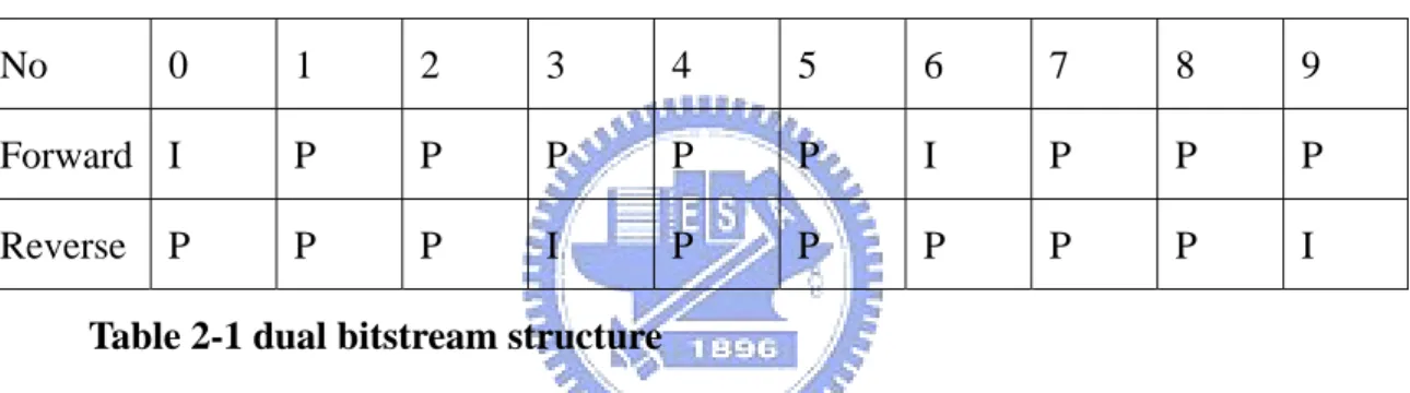
In [3], other previous work uses dual bitstreams structure to each sequence. One is encoded by forward playback sequence and another is encoded with reverse playback

sequence. For example, we encode a sequence with 9 frames which shows in Table 2-1. With 2 bitstream, the client requests a frame to server. The server finds the shortest way to get the frame. For example, if the client want to get 6th frame, the server pare the forward bitstream because it just need to parse 1 frame then the client can get the target frame. If we want get 5th, first we parse the 6th I frame of the forward bitstream and parse the 5th motion vector and residue of the reverse bitstream and then we can get the 5th frame.

This algorithm must contain 2 bitstreams and sometimes it needs to switch different bitstream to go minimum path to get target frame so it may not match perfectly.

No 0 1 2 3 4 5 6 7 8 9

Forward I P P P P P I P P P

Reverse P P P I P P P P P I

Table 2-1 dual bitstream structure

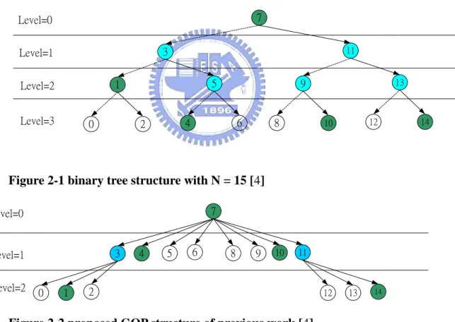
For VCR functionalities implementation with lower complexity and lower buffer cost, [4] reconstructs a new GOP structure. It decomposes sequential structure to hierarchical structure that can strongly reduce reference dependency. First, they present a binary tree structure which shows in Figure 2-1. Figure 2-1 uses a binary tree structure with N = 15, the level value is the same as reference dependency. From the Figure 2-1, the maximum dependency is 3, which is much smaller than the normal IPPP structure. The maximum dependency is reduced from N to log2 (N)

With the dependency reduction, random access functionality is easy to implement. From Figure 2-1, we can also found that there is no redundant frame decoding with 2n speed up (forward / inverse) playback because we can just skip large level frames. But this structure can not supply non 2n speed up playback.

GOP structure shows in Figure 2-2. It sets the center frame to be the first encoded frame. The frame of level = n connect to the edges of level = n-1 and each level has the same frame number. Comparing Figure 2-1 and Figure 2-2, if we want triple speed up playback that display frame 1, 4, 7, 10, and 14, which is green color in figure, the redundant decoded frame of binary tree are 5 frames, including 3, 5, 9, 11, and 13. But for the Figure 2-2 structure only has 2 redundant frames, which is frame 3 and 11.

Figure 2-1 and Figure 2-2 structures supplies much faster random access and fast playback with fewer redundant frames. But in this paper, it has not implemented the structure so we do not know the coding efficiency. Further, in this paper only one direction prediction is considered, bi-direction prediction is not discussed in this paper.

0 1 2 3 4 5 6 7 8 9 10 11 12 13 14 Level=0 Level=1 Level=2 Level=3

Figure 2-1 binary tree structure with N = 15 [4]

7 3 5 6 8 9 11 0 1 2 12 13 14 Level=0 Level=1 Level=2 4 10

2.2 Advanced Video Coding

Advance Video Coding (AVC), unlike the previous video coding standard such as MPEG-2, provide a flexible reference picture management and utilization scheme. We utilize this scheme to achieve our tree-like prediction structure. In section 2.2.1 we provide an overview of AVC. In Section 2.2.2, we describe the concept and syntax of the reference picture management and utilization scheme in AVC.

2.2.1 Overview

AVC is the newest video coding standard developed by the Joint Video Team (JVT) of ISO/MPEG and ITU. It provides better coding efficiency compare with MPEG-4 and H.263. The detail syntax and decoding method are described in [7]. In the following, we firstly briefly described the AVC encoding process, and then briefly describe some highlighted features in AVC that enables enhanced coding efficiency.

In AVC encoding process, a video sequence is separate into several pictures, and each picture will be processed macroblock by macroblock.

Figure 2-2 is the AVC encoder block diagram. In inter prediction mode, it use block-based motion estimation and motion compensation to generate the prediction image. In intra prediction mode, is use the previous coded macroblocks at the same picture to generate the prediction image. The best prediction mode is selected by the mode decision scheme. The prediction value of the best prediction mode is subtracted from the original image to form the prediction residue (Dn). DCT and quantization are then applied on the residue. The results are further entropy coded to generate the bitstream. The reconstructed pictures are then generated in reverse direction of encoding, and are stored in the reference picture buffer. It will be used for the inter prediction of the following pictures.

Figure 2-3 AVC encoder [7]

Compare with the previous video coding standard, such as MPEG-2, the AVC has the following new features that can improve the coding efficiency: [8].

z Variable block size motion compensation with small block size: AVC support

seven different block size, range from 4x4 to 16x16.

z Quarter sample accurate motion compensation: the prior standards just enable

half sample motion vector accuracy.

z Motion vectors over picture boundaries: the picture boundary extrapolation

technique is first used in H.263 and is included in AVC.

z Weighted prediction: this can dramatically improve coding efficiency for light

change in the same scenes.

z Small block size transform: in prior standards use transform block size of 8x8,

but AVC use block size of 4x4 transform that allows encoder to represent signal more locally-adaptive.

z Exact-match inverse transform: in previous standard, the DCT transform and

and inverse transform are perfect reconstruction.

z Arithmetic entropy coding: a powerful arithmetic coding method known as

CABAC is adopted in AVC. We can choose CAVLC and CABAC for entropy coding.

z Context-adaptive entropy coding: The two entropy coding method adopted in

AVC, CAVLC and CABAC, are both use context-based adaptive to improve performance.

Except the above features, AVC also provides a flexible reference picture management and utilization scheme, which is strongly related with our work. The detailed descriptions are given in the following section.

2.2.2 Reference picture management process

The reference picture management scheme in AVC can be generally classified as following [8]:

z Multiple reference picture motion compensation: there is only 1 reference

picture in forward prediction and 2 reference pictures in bi-direction prediction in prior standards. In AVC, we can use 16 reference pictures at most.

z Decoupling of referencing order from display order: in prior standards, the

encoding order has strict limitation. In AVC, it removes the restriction that the encoder can choose the order of pictures with high degree of flexibility. z Decoupling of picture representation methods from picture referencing

capability: in prior standards, bi-direction picture can not be used as reference for prediction, but AVC remove the restriction that bi-direction picture can be used as reference.

management [7]. All of their related syntax is stored in the slice header of each slice, so the decoder can find out the temporal dependency of each picture by only decode the slice header rather than the whole picture.

2.2.2.1 Reference picture list initialization process

Previous video codec such as MPEG4 contains only one forward reference picture for P-picture, or one forward and one backward reference picture for B-pictures, so it is unnecessary to control the reference picture order. In AVC, the reference picture number can be up to 16. AVC uses the “reference picture list” to list the reference pictures that can be used by the handling pictures. Each index of the reference picture list mapped to a reference picture inside the decoded picture buffer (DPB). During the motion estimation (ME) and motion compensation (MC) stage of an inter-predicted block, the block simply indicate the index of the reference picture list to point out which reference picture it is used. With this structure, the AVC standard must provide a mechanism to “order” the reference pictures in the reference picture list, that is, which reference picture is put at which index inside the reference picture list. The “reference picture list initialization process” provides the default ordering method in AVC.

In AVC, the reference pictures are divided into two types, one is short term reference pictures and another is long term reference pictures, each of which has different management method. To each short-term reference picture a variable PicNum is assigned, and to each long-term reference picture a variable LongTermPicNum is assigned. During the memory management process in AVC, one can identify a short-term or a long-term reference picture with PicNum or LongTermPicNum, respectively. For short term reference frame, PicNum is generally set with a value that related to the display order of that frame. For long-term reference frame, LongTermPicNum is set with the “memory management control operation” (MMCO) in

AVC, we will describe its detail in section 2.2.2.3.

In the following, we describe the reference picture list initialization process for P slice and B slice.

P slices reference list initialization

For P slice, the reference picture list RefPicList0 is ordered such that the short-term reference frames has lower indices than long-term reference frames. For short-term reference frames, they are ordered starting with the one that has the largest PicNum to the one that has the smallest PicNum. For long-term reference frames, they are ordered starting with the one that has the smallest LongTermPicNum to the one that has the largest LongTermPicNum.

We give an example for P slices list initialization:

Assuming we have 5 reference frames that contain 3 short term reference frames with PicNum = 303, 302, 300 and 2 long term reference frames with LongTermPicNum = 0 and 3. After the initialization,

RefPicList0 [0] is the short term reference picture with Picnum = 303 RefPicList0 [1] is the short term reference picture with Picnum = 302 RefPicList0 [2] is the short term reference picture with Picnum = 300

RefPicList0 [3] is the long term reference picture with LongTermPicnum = 0 RefPicList0 [4] is the long term reference picture with LongTermPicnum = 3

B slices reference list initialization

For B slice, the reference picture is also ordered such that the short-term reference frames has lower indices than long-term reference frames. For the short term reference frames, we further divided them into two parts. The first part contains all references whose PicNum are smaller than current PicNum and the second part contains all

references whose PicNum are larger than current PicNum. The first part short-term reference frames are ordered starting with the one that has the largest PicNum to the one that has the smallest PicNum. The Second part short-term reference frames are ordered starting with the one that has the smallest PicNum to the one that has the largest PicNum.

For reference picture list RefPicList0, it is started with the entire ordered short-term reference frame in the first part short-term reference, followed by the entire ordered short-term reference frame in the second part, finally is the long-term reference frames with the same order used in P slice. For reference picture list RefPicList1, it is started with the entire ordered short-term reference frame in the second part short-term reference, followed by the entire ordered short-term reference frame in the first part, finally is again the long-term reference frames with the same order used in P slice. Also note that after this ordering, if the RefPicList1 is identical with RefPicList0, the first two entries of RefPicList1 are switched.

We also give an example to B slice:

Assuming we have 6 reference frames that contain 4 short term reference frames with Picnum = 303, 302, 300, 299 and 2 long term reference frames with LongTermpicnum = 0 and 3. The current reference frame is 301. After the initialization,

RefPicList0 [0] is the short term reference picture with Picnum = 300 RefPicList0 [1] is the short term reference picture with Picnum = 299 RefPicList0 [2] is the short term reference picture with Picnum = 302 RefPicList0 [3] is the short term reference picture with Picnum = 303

RefPicList0 [4] is the long term reference picture with LongTermPicnum = 0 RefPicList0 [5] is the long term reference picture with LongTermPicnum = 3 RefPicList1 [0] is the short term reference picture with Picnum = 302

RefPicList1 [2] is the short term reference picture with Picnum = 300 RefPicList1 [3] is the short term reference picture with Picnum = 299

RefPicList1 [4] is the long term reference picture with LongTermPicnum = 0 RefPicList1 [5] is the long term reference picture with LongTermPicnum = 3 2.2.2.2 Reference picture list reordering process

In 2.2.2.1 we introduce the initialization of the reference list. The initialization process order the short term reference pictures such that the temporally closer reference frame is in lower index of the reference list. This is because temporally closer reference frames usually provided better prediction image and will be encoded many times for each inter prediction block. In the AVC entropy coding method such as CABAC, lower reference picture index can be coded with fewer bits, so put temporally closer frame at lower index can provide better coding efficiency. On another side, the initialization process order the long term reference frames from smallest LongTermPicNum to largest LongTermPicNum, which can not reflect to the frequency of there utilization. Further, sometimes the temporally closer reference frame is not the best reference frame and we will want to reorder the reference picture list. Another reason that we need to reorder the reference picture list is, for some prediction structure, such as the proposed tree-prediction structure, we may need to move some reference pictures outside the scope of the temporal prediction process of the handling picture to reduce the temporal dependency. To address these issues, AVC provides the reference picture list reordering process to make the user can fully control the order of the reference picture list.

In reference buffer list section, AVC has 2 reference buffer lists. If we just use forward prediction, the RefPicList0 is used. If we use forward and backward prediction at the same time, RefPicList1 and RefPicList0 buffers are both used. We use ref_pic_list_reordering_1X syntax element to present which buffer we are control. If ref_pic_list_reordering_flag_10 = 1, we make refPicList0 buffer reordering and if

ref_pic_list_reordering_flag_11 = 1, we make refPicList1 buffer reordering.

The second syntax element: reordering_of_pic_nums_idc. If reordering_of_pic_nums_idc = 0 or 1, our reordering process of reference buffer lists are for short term reference frame. If reordering_of_pic_nums_idc = 2, our reordering process of reference buffer lists are for long term reference frames. If reordering_of_pic_nums_idc = 3, the reference reordering function ends.

If reordering_of_pic_nums_idc = 0, we parse abs_diff_pic_num_minus1[i] = k that we move the reference of pic_num = ( current pic_num - abs_diff_pic_num_minus1[i]) to the kth order of reference list.

If reordering_of_pic_nums_idc = 1, we parse abs_diff_pic_num_minus1[i] = k that we move the reference of pic_num = ( current pic_num + abs_diff_pic_num_minus1[i]) to the kth order of reference list.

If reordering_of_pic_nums_idc = 3, we parse long_term_pic_num[i] = k that we move long_term_pic_num[i] to the kth order of reference list.

We make a long term reference reorder example in here. We have reference 0, 1, 2 with long term number = 0, 1, 2. The original reference list order is 0, 1, and 2. We want to reorder the reference list in inverse order. In this case, we want move long term number = 2 to 1st order and 0 to the end. So 1st we set long_term_pic_num[2] = 0 that the reference list order become 2, 0, 1. Then we set long_term_pic_num[1] = 1 that the reference list order become 2, 1, 0.

2.2.2.3 Reference picture list marking process

In the previous video coding standard such as MPEG-2, the reference frame is only the temporally closest one. In AVC, it simply set the limitation of the reference picture number. Which reference picture are going to be stored to or remove from the reference picture buffer can be fully controlled by the encoder, as long as it has not

exceed the reference picture number limitation. In AVC, the “reference picture list marking process” is the tool to handle these matters. There are two method of marking process, one is “sliding window” and the other is “adaptive memory control”

The basic memory management method of AVC is sliding window marking process. It will be invoked if we have not use the adaptive memory control marking process. When the handling picture is set as a reference picture, sliding window marking process will put this picture into the reference picture buffer. If the reference picture buffer is full, it remove the oldest reference frame in encoding order from the reference picture buffer.

Different with the sliding window marking process, adaptive memory control marking process make the encoder can fully control which picture will be store to or remove from the reference picture buffer through the “memory management control operation” (MMCO) command. As our tree prediction structure needs to utilize the adaptive memory control marking process, we described the six MMCO commands provided in AVC in the following.

If memory_management_control_operation = 1, this operation marks short term reference frames as unused for reference that means we remove the short term reference frame from reference buffer. This operation includes 3 parameters which are picNumX, CurrPicNum and difference_of_pic_nums_minus1.

Every reference frame has its identification number and the picNumX means its identification number. CurrPicNum is the picNumX of the current frame. The parameter difference_of_pic_nums_minus1 is used as function parameter. If we set MMCO(we use this to instead memory_management_control_operation) = 1, we must pass difference_of_pic_nums_minus1. From the inner operation: picNumX = CurrPicNum – (difference_of_pic_nums_minus1+1) we can calculate picNumX, and then we drop the reference frame with id number = picNumX.

If MMCO = 2, this operation marks long term reference frame as unused for reference that we remove the long term reference frame from reference buffer. We control the long term reference frame by long term number so we sent the long term number and mark that reference frame as unused.

MMCO = 3, this operation assigns long term number to short term reference frame. In AVC software, if we do not use MMCO it always sets reference frame as short term reference frame at first and if we want to use long term reference frame, we can use this operation to make the frame from short term reference frame to long term reference frame. In this operation, we must pass 2 syntax elements: difference_of_pic_nums_minus1 and LongTermFrameIdx. The first element is introduced in MMCO = 1 section, we use that to get the short term reference frame id number and then we set this frame as long term reference frame with long term number = LongTermFrameIdx. One important thing in here that if the long term number is used in the other long term reference frame, the new long term reference frame will use the long term number and the old one is removed from the long term reference buffer.

MMCO = 4, this operation sets the maximum long term frame index. We change the maximum index value of long term reference frame in this operation. We need only one syntax element: max_long_term_frame_idx_plus1. If the long term number of any long term reference frame is greater than (max_long_term_frame_idx_plus1-1), the reference frame shall be marked as unused for reference so if max_long_term_frame_idx_plus1 = 0 and then there will be no reference frame in the long term reference buffer.

MMCO = 5, this operation marks all reference frame as unused for reference frame and set maximum long term frame index as no long term reference frame. This operation is like reset all reference setting. It cleans all reference buffers which include long term and short term buffer to null.

MMCO = 6, this operation assigns long term frame index to the current frame. We must pass one syntax element LongTermFrameIdx as long term number of current frame. If the long term number is used in the other reference frame, we remove the old reference frame as unused like we describe in MMCO = 3.

Finally we introduce MMCO = 0, this operation means that the MMCO is over. We use this operation when we have done all MMCO instructions.

We make a MMCO example, if we have 0, 1, 2, 3, total 4 frames and we set 0th as long term number = 0, 1st as long term number = 1, 2nd as long term number = 2, 3rd as long term number = 0.

First, we want to set 0th as long term number = 0, there are two methods. 1st we can set img->long_term_reference_flag = 1. This function can set I_slice frame as long term frame with long term number = 0. 2nd we use MMCO operation but MMCO can not use if the frame is I_slice so we must define MMCO at the 1st picture.

At the 1st picture, we see that the maximum of our long term number is 3 so we define our long term buffer size = 3. We use MMCO = 4 and give max_long_term_frame_idx_plus1 = 3 .want set 0th as long term number =0.

Then we want to set 0th with long term number = 0. We use MMCO = 3 and difference_of_pic_nums_minus1 = 0 and long_term_frame_idx =0.

And then we set the current frame with long term number = 1. We use MMCO = 6 and long_term_frame_idx = 1.

Finally we set MMCO = 0 to end the MMCO loop. The 2nd picture just set MMCO = 6 and long_term_frame_idx = 2 and next MMCO = 0.

The 3rd picture set as long term number = 0, it replaces 0th picture. MMCO = 6 will remove the long_term_frame_idx long term picture and then set the current picture with long term number = long_term_frame_idx.

Chapter 3

Tree Architecture Coder

In this chapter, we describe the proposed symmetric tree prediction structure. Firstly, we describe the basic concept of the proposed architecture in section 3.1. Then, we describe the implementation of the symmetric tree prediction structures in AVC encoder in section 3.2. We then described the decoding method that supports VCR functionalities in section 3.3. Finally, in section 3.4, we discuss the decoding complexity of various VCR functionalities for various GOP structures, including the normal GOP structures and the proposed symmetric tree prediction structures.

3.1

Basic Concept of Our Tree

Prediction Structure

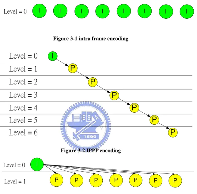
In the traditional video reorder, the pictures are directly stored in the video cassette without prediction, just as shown in Figure 3-1. In this architecture, the video player can access and display any pictures without access any other pictures. Thus the VCR functionalities can be easily achieved. This is similar with digital video compression that does not allowed temporal prediction. However, digital video compression usually utilizes temporal prediction to remove the temporal redundancy and thus dramatically increase the coding efficiency. Figure 3-2 shows commonly used prediction architecture in video compression. Every picture is predicted by the previous pictures to remove the temporal redundancy between them. However, this architecture causes difficulties on VCR functionalities. For example, if we want to access the latest pictures, the decoder needs to decode all the previous pictures to derive the correct prediction image that used

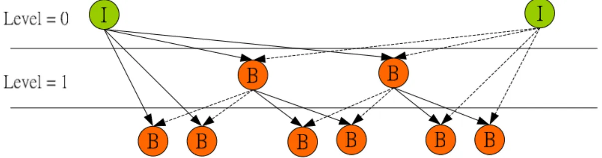
to reconstruct the latest pictures. Figure 3-3 shows a different prediction structure that utilizes temporal prediction and also provide the convenience for VCR functionalities: Every picture is temporally predicted by the first picture. Comparing to Figure 3-1, it has inter prediction that provides better coding efficiency. But with the inter prediction, it also cause one more delay for random access except the first frame. Comparing to Figure 3-2, the average distance of the inter prediction is longer so the coding efficiency is worse but the random access functionality is much better.

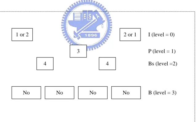
In Figure 3-4, we extend the concept in Figure 3-3 into “multiple levels”. In Figure 3-3, the pictures in level 1 is predicted by the picture in level 0. In Figure 3-4, the reference picture is restricted by the following rule:

Rule 1: A pictures in level i can only be predicted by the pictures in level j, where j<i.

Compare with Figure 3-3, it reduce the distance of inter prediction and hence improve the coding efficiency. However, if we have not assigned the reference picture correctly, it will also significantly increase the random access decoding delay. For example, assuming the picture in level 2 can be predicted by any picture in level 0 and 1, than we need to decode all of these pictures before we can corrected decode the picture in level 2. To solve this problem, we add the following rule to restrict the usage of the reference picture.

Rule 2: Only the temporally closest picture can be used as reference. The reference picture of the reference picture can also be taken as reference picture.

For example, frame 9 can take frame 8 and frame 12 as reference, because there are temporally closest picture at lower level. It can also take frame 0 as reference, because frame 0 is the reference picture of frame 8. Frame 9 can not take frame 4, 16, 20, and 24 as reference because they violate rule 2, and hence reduce the decoding delay of this structure. With this 2 rule, we form a hierarchical prediction structure. If

we inspect this structure only from one prediction direction, that is, forward or backward, it is just like a tree, so we can call this structure as “tree prediction structure”.

Another feature of the structure in Figure 3-4 is it symmetry ⎯ Firstly the prediction structure is symmetric between forward direction and backward direction. That is, the decoding complexity is identical for forward playback or backward playback. Secondly, in each level the picture number of each sub-group, which can also be viewed as the number of the “branch” number in a tree, are identical. For example, each sub-group in level 1 contains two pictures, which are frame 4 and frame 8, or frame 16 and frame 20. Each sub-group in level 2 contains three pictures, which is frame 1 to frame 3, frame 5 to frame 7, etc. Because the frame in each level can only reference the frame at lower level, and then fast forward and fast backward can be achieved easily at decoder. For 2x speed up, the decoder can simply drop all the odd frames. For 4x speed up, the decoder can drop the entire picture in level 2 and only decode the picture in level 0 and level 1. For 12x speed up, the decoder can drop the entire picture in level 1 and 2 and only decode the picture in level 0.

We name the structure in Figure 3-4 as “symmetric tree prediction structure”, a tree prediction structure that is symmetric. It enables all the required VCR functionalities with low complexity at decoder: low-delayed random access, low complexity forward and backward playback, simple fast playback.

Tree prediction structure is not restricted to be symmetric. For example, we show an unrestrained tree in Figure 3-5. The tree in Figure 3-5 still obey rule 1 and rule 2, but the branch number in each level are different with each other. With this flexibility, tree prediction structure can be adapted with the temporally local statistic of the sequence and hence improve the prediction efficiency. However, without symmetry, the tree in Figure 3-5 is difficult to provide VCR functionality. For example, we can not simply drop the odd pictures to provide a 2x speed up, because they could be the reference

pictures of the remaining even pictures. Therefore, in this thesis, we will focus on the “symmetry tree prediction structure”, such as shown in Figure 3-4.

Figure 3-1 intra frame encoding

Figure 3-2 IPPP encoding

Figure 3-4 Prediction method for the nearest level

Figure 3-5 An example of a PGOP with various descendent picture number and depth. Each circle indicates a picture. The black circle is the root I-picture.

The red circles are the PIDR-pictures. The green circles are the leaf pictures.

Level 1 Level 2 Level 3 Level 4 Level 5 PGOP

3.2

Symmetric Tree Structure Encoder

Implementation in AVC

From the previous section, we know that symmetric tree prediction structure is more suitable to generate a bitstream that can easily support VCR functionality. In this section, we describe the implementation of our symmetric tree prediction structure in AVC encoder.

To easily express our symmetric tree prediction structure, the following notation is used:

GOPSize_LevelX-PictureType-BranchNumber-ReferencePictureNumber

“GOPSize” is picture number in a GOP. For example, a GOP with 16 pictures is denoted as N16. “PictureType” is the picture type of the specified level. “BranchNumber” means the picture number between the two nearest lower-level pictures at the specified level. We call it “branch” because these pictures are just like the branch in a tree. For example, in Figure 3-6 the branch number for level 1, 2, and 3 are 1, 1, and 3, respectively. We combine the “PictureType” and “BranchNumber” to make the expression more compact. For example, “B3” means there are 3 branches in this level, each of which has “B” picture type. “ReferencePictureNumber” is the reference picture number used for pictures in the specified level, and the reference picture number for forward reference and backward reference will be shown separately. For example, F1B1 means 1 forward reference and 1 backward reference.

For example, we can denote the symmetric tree GOP structure in Figure 3-6 as N16_P1F2_B1F1B1_B3F1B1, which means the there are 16 pictures in this GOP (N16). In level 1, P1F2 means there is only one picture with picture type P, and it has 2 forward

references. In level 2, B1F1B1 means there is only one picture with picture type B, and it has 1 forward reference and 1 backward reference. In level 3, B3F1B1 means there are 3 pictures with picture type B, and they have 1 forward reference and 1 backward reference. Further, sometimes when we are not focus on the reference picture number, and we can remove the related field in the above notation and, for example, Figure 3-6 is then expressed as N16_P1_B1_B3. With this notation, we use an example to describe the implementation of the symmetric tree prediction structure encoder in AVC.

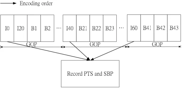
Encoder implementation of the symmetric tree prediction structure: N16_P1_B1_B3 As shown in Figure 3-6 we show a GOP which contain 16 pictures. Level 1 has 1 branch with P picture type. Level 2 also has one branch but with B picture type. The third level has 3 branches with B picture type. With the picture type and branch number in each level, we can then derive the encoding order, as shown in Figure 3-7. For example, frame 8 is P-picture, so we only need to encode the forward reference picture, which is frame 0, before encoding it. However, Frame 4 is B-picture, and we need to encode both its forward and backward reference, which is frame 0 and frame 8 respectively, before encoding it. With this concept we can generate the encoding order of this GOP and start the encoding process.

During the encoding of each picture, we need to control the reference picture reordering process and the marking process to achieve the symmetric tree prediction structure we want. Figure 3-8 shows the long term picture numbers (LTPN) setting. In the symmetric tree prediction structure, we restricted the reference picture to the temporally closest picture at the lower level. Therefore in a certain level, only two pictures will be used as reference at the same time. We can allocate two LTPN to each level, and all the pictures in the same level can recycle these two LTPN. For example, we allocate LTPN 1 and 2 to level 0. We can assign LTPN=1 for frame 0, LTPN=1 for frame 16 and then reuse LTPN=1 for frame 32 and LTPN=2 for frame 48… When there

is only one branch in a level, we can only allocate one LTPN to that level. This is because with one branch in a level, only one of the “two temporally closest reference picture” is at the specified level, and another is at the lower level, such that it will only consume one LTPN a certain time. For example, we can assign LTPN=3 for frame 8 and LTPN=4 for frame 4 and 12.

In Table 3-1, we show the reference picture list after initialization and after reordering of each picture. Because we are using long-term reference picture, the initialize process will put the long-term reference picture that has smallest LTPN at lower index. We then reorder the list such that the temporally closer picture will allocate at lower index. In this way the closer picture, which is usually the frequently used picture, can be entropy encoded more efficiently. The reordering process also need make sure the reference picture that violate the rule 1 and rule 2 described in section 3.1 will not appear in the reference picture list of the handling frame. We also show the reference picture marking process and the reference picture list after the marking process of each picture. It reflects the LTPN assignment that we discussed in the previous paragraph.

Figure 3-7 Coding order for GOP structure N16_P1_B1_B3

Figure 3-8 long term picture numbers setting for GOP structure N16_P1_B1_B3

I (level = 0) P (level = 1) Bs (level =2) B (level =3) 0 9 1 2 10 3, 4, 5 6, 7, 8 11 12 13 14 15 16 I (level = 0) P (level = 1) Bs (level =2) B (level = 3) 1 or 2 2 or 1 3 4 4 No No No No

Table 3-1 reference picture list of each picture of GOP structure N16_P1_B1_B3 Coding order Frame number (display order)

Level List after initialization

List after reordering

Picture marking process

Picture in buffer after marking process. (Format: frame number (LTPN*) 0 0 0 Set Frame0 LTPN=0 0(0) L0: 0 L0: 0 1 8 1 L1: - L1: - Set Frame8 LTPN=3 0(0), 8(3) L0: 0, 8 L0: 0, 8 2 4 2 L1: 8, 0 L1: 8, 0 Set Frame4 LTPN=4 0(0), 8(3), 4(4) L0: 0, 8, 4 L0: 0, 4, 8 3 1 3 L1: 8, 0, 4 L1: 4, 8, 0 None 0(0), 8(3), 4(4) L0: 0, 8, 4 L0: 0, 4, 8 4 2 3 L1: 8, 0, 4 L1: 4, 8, 0 None 0(0), 8(3), 4(4) L0: 0, 4, 8 5 3 3 L0: 0, 8, 4 L1: 8, 0, 4 L1: 4, 8, 0 None 0(0), 8(3), 4(4) L0: 0, 8, 4 L0: 4, 0, 8 6 5 3 L1: 8, 0, 4 L1: 8, 4, 0 None 0(0), 8(3), 4(4) L0: 0, 8, 4 L0: 4, 0, 8 7 6 3 L1: 8, 0, 4 L1: 8, 4, 0 None 0(0), 8(3), 4(4) L0: 0, 8, 4 L0: 0, 8 8 7 3 L1: 8, 0, 4 L1: 8, 0 None 0(0), 8(3), 4(4) L0: 0, 8, 4 L0: 9 16 0 L1: 8, 0, 4 L1: Set Frame16 LTPN=1 0(0), 16(1),8(3),4(4) L0: 0, 16, 8, 12 L0: 8, 0, 12, 16 10 12 3 L1: 16, 0, 8, 12 L1: 12, 16, 8, 0 Set Frame12 LTPN=4 (remove Frame4 automatically) 0(0), 16(1), 8(3), 12(4) L0: 0, 16, 8, 12 L0: 8, 0, 12, 16 11 9 3 L1: 16, 0, 8, 12 L1: 12, 16, 8, 0 None 0(0), 8(3), 12(4) L0: 0, 16, 8, 12 L0: 8, 0, 12, 16 12 10 3 L1: 16, 0, 8, 12 L1: 12, 16, 8, 0 None 0(0), 8(3), 12(4) L0: 0, 16, 8, 12 L0: 8, 0, 12, 16 13 11 03 L1: 16, 0, 8, 12 L1: 12, 16, 8, 0 None 0(0),16(1), 8(3), 12(4)

L0: 0, 16, 8, 12 L0: 12, 8, 0, 16 14 13 3 L1: 16, 0, 8, 12 L1: 16, 12, 8, 0 None 0(0),16(1), 8(3), 12(4) L0: 0, 16, 8, 12 L0: 12, 8, 0, 16 15 14 3 L1: 16, 0, 8, 12 L1: 16, 12, 8, 0 None 0(0),16(1), 8(3), 12(4) L0: 0, 16, 8, 12 L0: 12, 8, 0, 16 16 15 3 L1: 16, 0, 8, 12 L1: 16, 12, 8, 0 None 0(0),16(1), 8(3), 12(4)

3.3

Decoder implementation that

support VCR functionalities

The bitstreams generated by our encoder that described in section 3.2 is compliant with AVC standard and can be correctly decoded by the AVC standard compliant decoder. However, a normal AVC decoder, such as the reference decoder provided in [9], can only decode the bitstream with forward display. To provide the VCR functionalities such as backward display, fast forward/backward display, and random access, we need to redesign the decoder.

The basic structure of our AVC decoder that supports VCR functionality is to provide an efficient decoding method for random access, and then all the VCR functionality such as fast forward and fast backward can be easily support. From section 2.2, we know that the slice header of each slice in the sequences contain all the reference information. Therefore for efficient random access, we only need to parse the slice header of the sequences to generate the GOP structure of each GOP, and then we know the dependency among pictures. A size configurable GOP structure buffer is used to store the GOP structure, thus we don’t need to parse and decode the slice header if the related GOP structure is already in the buffer. With the knowledge of the dependency, we can generate the reference picture for the request picture. A size-configurable picture buffer is used to store the decoded picture such that we don’t need to decode the recently decoded picture again and again. The detail of our decoder is described as the following, and Figure 3-10 shows the decoder flow chart.

1st step: Decoder initialization. Parse the picture order count (POC) related syntax in the slice header of the entire the bitstream, record the playback time stamp (PTS) and start byte position (SBP) of the first picture (in display order) in each GOP.

We show the diagram in Figure 3-9.

2nd step: Get the request target PTS from the player. The decoder find out the GOP which the target PTS belong to. If the target GOP structure has not recorded in the “GOP structure buffer” (GSB), go to step 3. Else go to step 4.

3rd step: Derive the GOP structure. Parse the entire slice headers in this GOP. Derive the reference pictures list of each picture in this GOP. Store the GOP structure information in the GSB. If the GSB is full, remove the data of the GOP that is farthest (in display order) from the current GOP.

4th step: If the target picture can not be found in “picture buffer” (PB), go to step 5. Else go to step 8.

5th step: Check the required reference pictures of the target picture. If some reference pictures of the target picture are not available in the PB, go to step 6. Else go to step 7.

6th step: Decode the reference pictures that required of the target picture, stored it in the PB. If the PB is full, the picture on the PB is removed with the following order: 1. Remove the picture that is in different GOP. 2. In the current GOP, remove the picture that has highest level ID and is farthest (in display order) from the target picture.

7th step: Decode the target picture, stored it in the PB. If the PB is full, the same method used in step 6 is used to remove the picture in PB.

8th step: Send the target picture memory position to the player. Go to step 2, wait for the decoding request of the next picture from the player.

3.4

Cost of VCR Functionalities

for Various GOP Structures

In this section we compare the cost of VCR functionalities for various GOP structures. In 3.4.1, we discuss the cost of forward and backward playback for normal GOP structure. In 3.4.2, the same analysis is applied on the proposed symmetric tree prediction structure with B-picture only. We further discuss the difference of B and P picture type in the symmetric tree prediction structure. Finally, the cost of fast playback and random access for various GOP structure are discussed in 3.4.4.

3.4.1 Cost of forward and backward playback for

normal GOP structure

We firstly discuss the normal GOP structure with M=1, as shown in Figure 3-2. Assuming it has GOP size N = 16 and use 3 reference frames. In Figure 3-11 we show the decoding order and decoding delay for forward playback in one GOP. X-axis is frame numbers and Y-axis is time orders. Each time unit is identical with the duration of display one frame. We also assume that decode one frame need one time unit. There are four colors to present 4 different situations: Red color means the specified frame is under decoding. Cyan color means it is put into the reference frame buffer. Blue color means it is under displaying. And yellow color means it is used as reference frame for other frames. In forward display, this GOP structure works well, there is no delay between decoding and displaying each frame.

decoder must decode the entire frame in this GOP before it can display the first requested frame, which is the frame N-1. Such that we can see the delay of backward playback is equally to the GOP size N. Because there is unlimited buffer size, the decoder can store every decoded frame during the decoding, and it can display frame N-2, frame N-3, … , to frame 0 with load them from the decoder buffer rather than decode them again. When the decoder buffer size is limited, the backward playback delay becomes even worse. Due to there are 3 reference frame, the minimum buffer size is 3. For inverse playback, the decoder firstly decode the entire GOP to gets the final pictures of the GOP, which is frame N-1, and then it can display frame N-1 as well as frame N-2 and frame N-3, because frame N-2 and frame N-3 are also stored in the frame buffer. Next, the decoder have to decode the bitstream from frame 0 to frame N-4 again to get frame N-4, and display frame N-4 to frame N-6. Consequently, we can found that overall the backward playback with buffer size = B needs to decode

N+ (N-B) + (N-2B) + … = (NxN)/(2xB) frames. With this example we know that for IPPP GOP structure, if the GOP size is large, the decoder cost for backward playback is very high.

We now discuss the decoding delay of normal GOP structure with M=4, as shown in

Figure 3-13. Again assume the GOP size N=16 and there are 3 reference frames.

Similar with M=1, there is no decoding delay for forward playback. In Figure 3-15, we show the decoding delay of backward playback with unlimited decoder buffer size. Compare with M=1, the backward decoding delay of M=4 is much smaller. Instead of decode the entire GOP, it only need to decode the frames that are used as reference, which is frame 0, M, 2M, … N. And hence the decoding delay is N/M. If the decoder buffer size is limited, the inverse playback will also cost more delays. Similar with M=1, assuming buffer size = B, we can found the overall decoding delay is N/M + (N/M-B) + (N/M-2B) … = (N/M)x(N/M)/(2xB).

In normal GOP structure, we can found that larger M can reduce the decoding delay of backward playback. However, the delay is still a linear function of the GOP size N. Therefore with normal GOP structure, we must use smaller N to prevent problem in VCR functionality. However, with the frequently used intra frame, the coding efficiency is limited.

3.4.2 Cost of forward and backward playback for

symmetric tree prediction structure with different

level depth

In this section, we discuss the decoding delay of the proposed symmetric tree prediction structure. From the previous section, we know that the backward playback decoding delay of normal GOP is a linear function of GOP size N. To prevent long delay at decoder side, one can not use large GOP size N and hence limited the coding efficiency. There is no such problem in symmetric tree prediction structure.

We give 2 examples of our symmetric tree prediction structure, as shown in Figure 3-16 and Figure 3-17. Figure 3-16 is a N16_B1_B7 structure; it demonstrates the symmetric tree prediction structure with fewer levels. Figure 3-17 is a N16_B1_B1_B1_B1 structure; it demonstrates the symmetric tree prediction structure with largest levels. Note that for convenience, we will use N16_4B1, which means 4 level depths and each level has one branch with B-picture type, instead of N16_B1_B1_B1_B1 in the following description. For B1_B7 structure, we show the decoding order and decoding delay for forward and backward playback in Figure 3-18 and Figure 3-19, respectively. For 4B1 structure, we also show the decoding order and decoding delay for forward and backward playback in Figure 3-20 and Figure 3-21, respectively.

Due it is symmetric for forward and backward prediction in symmetric tree prediction structure. So it costs identical delays for forward and backward playback.

The decoding delay computation of the symmetric tree prediction structure is very similar with the long-term picture number assignment described in section 3.2. Due to

the prediction rule described in section 3.1, for a certain level, only the temporally closest two pictures will be used to predict the frame in higher level. Which means we will increase 2 decoding delay with increasing one level. Further, when there is only one branch in a certain level, only one of the “two closest frames” is inside that level, and thus will only increase one decoding delay at that level. With this knowledge, it is easy to compute the decoding delay of B1_B7 and 4B1.

Considering the B1_B7 structure, level 0 will cause two delays. level 1 will cause 1 delay because there is only one branch. Therefore the maximum decoding delay is 3. Considering the 4B1 structure, level 0 will also cause 2 delays. Each level of level 1 to level 3 will cause 1 delay. Therefore the maximum decoding delay is 5. When the GOP size is larger, the benefit of symmetric tree prediction structure is more significant. Assuming we always use one branch of each level, we will have a log2(N)B1 structure, and the maximum decoding delay is 2+log2(N)-1. For example, with N=64, we can generate a 6B1 structure with maximum decoding delay equal to 7. We can also use larger branch number in each level to reduce the total level number, and hence reduce the decoding delay. Assuming we always use H-1 branches for each level, where H>2. Then we will have a logH(N)B(H-1) structure with maximum delay equal to 2x logH(N). For example, with N=64 and 7 branches in each level, we can construct a 2B7 structure with maximum delay = 4. Comparing with the “backward playback with unlimited decoder buffer size” of normal GOP structure with N=64, the M=1 structure need 64 decoding delay and M=4 structure need 64/4=16 decoding delay, both are significantly larger then the symmetric tree prediction structure.

Symmetric tree prediction structure not only benefit with lower decoding delay. It also prevent the requirement of the “large decoder buffer” when the decoder does not have enough power to decode the bitstream several times. For backward playback, if the decoder wants to decode the bitstream only one time, the required decoder buffer size is

identical with the decoding delays no matter it is normal GOP structure or symmetric tree prediction structure. This is because “decoding delay” means the decoded frame number. If we can store all of these decoded frames, then we don’t need to decode them twice. As we already shows that the symmetric tree prediction structure has much lower decoding delay, we know that symmetric tree prediction structure can also significantly reduce the decoder buffer size requirement if the decoder can not or does not want to decode the bitstream several times.

B B B B B B B B B B B B B B B I I Level=0 Level=1 Level=2

Figure 3-16 the shortest depth symmetric tree structure B1_B7 GOP

Figure 3-18 forward playback decoding diagram of B1_B7 GOP structure