應用於短距離高速無線通訊之傳送端前置等化器

全文

(1)國立交通大學電信工程學系碩士班碩士論文. 應用於短距離高速無線通訊之傳送端前置等化器. Transmitter Pre-equalization for High-Speed Short Range Wireless Communications. 研究生：陳柏任指導教授：高銘盛. 教授. 中華民國九十六年二月.

(2) 應用於短距離高速無線通訊之傳送端前置等化器. Transmitter Pre-equalization for High-Speed Short Range Wireless Communications. 研究生. ：陳柏任. Student：Bo-Ren Chen. 指導教授：高銘盛博士. Advisor：Dr. Ming-Seng Kao. 國立交通大學電信工程學系碩士班碩士論文 A Thesis Submitted to The Institute of Communication Engineering College of Electrical Engineering and Computer Science National Chiao Tung University In partial Fulfillment of the Requirements For the Degree of Master of Science In Communication Engineering Feb 2007 Hsinchu, Taiwan, Republic of China. 中華民國九十六年二月.

(3) 應用於短距離高速無線通訊之傳送端前置等化器. 研究生. ：陳柏任. Student：Bo-Ren Chen. 指導教授：高銘盛博士. Advisor：Dr. Ming-Seng Kao. 國立交通大學電信工程學系碩士班. 摘要本論文旨在簡化應用於高速短距無線通訊系統中的接收端架構。我們提供一個在傳送端解決多路徑干擾問題的方法。我們設計一個多路徑處理器以量測多路徑衰降的係數並且估測對傳送信號的 ISI。根據已經估測的 ISI，我們修改傳送信號的振幅，使接收信號與傳送信號有相同的極性以及數量。當 ISI 和傳送信號有同的極性時，我們可以適當修改臨界值以節省傳送能量。此外，因為在傳送端做等化，我們可以事先知道後續傳送信號的資訊。因此當目前傳送信號所產生的 ISI 和後續傳送信號有同的極性時，我們可以進一步修改臨界值以節省更多的傳送能量。因為在傳送端做了等化，因此接收機變得非常簡單。最後，我們提出系統的效能分析並討論此系統的相關問題。. i.

(4) Transmitter Pre-equalization for High-Speed Short Range Wireless Communications. Student：Bo-Ren Chen Advisor：Dr. Ming-Seng Kao. Institute of Communication Engineering National Chiao Tung University. Abstract. The purpose of this paper is to simplify the receiver structure in high-speed short-range wireless communications. We develop solutions to deal with multipath problem at the transmitter (TX). A multipath processor (MP) is designed to measure the multipath coefficients and estimate the amount of possible ISI on the transmitted signal. According to the estimated ISI, we modify the transmitted signal amplitude to make the received signals with desired polarity and magnitude. For saving transmitted power, we can modify the threshold significantly while ISI and the current data have the different polarity. By doing pre-equalization at TX, the information of the upcoming data could be known in advance. We could also modify the threshold for saving more power by considering this information. Because equalization is done at TX, the receiver structure can be rather simple. We present the system performance analysis and discuss related issues of this system.. ii.

(5) 誌謝首先要感謝指導教授高銘盛教授，在我兩年的研究所生涯給予耐心的指導及啟發，並且也給予我一些人生價值觀上的思考。在論文寫作的過程中，所給我的幫助及建議，也使我受益匪淺。此外感謝實驗室的萬信學長，謝謝你在此論文上所給予的指導及幫助，謝謝書宗學長在兩年的研究所生涯給我的鼓勵。謝謝士瑋同學在研究所準備期間以及研究所生涯中的鼓勵及幫助。也謝謝大源，博文，韋強，琇云，志帆學弟妹們，研究所的生活有你們的參與，這些都會是我未來美好的回憶。馥慈，謝謝你，你是我研究所兩年的生活最大的支柱。最後謝謝我的父母及家人，謝謝你們在我最灰心的時候仍給予我鼓勵及支持。在此，謹將本篇論文獻給我的父母以及關心我的親友們。. iii.

(6) Contents List of Figures………………………………………………........................2 List of Tables………………………………………………………………..3. Chapter 1 Introduction…………………………………………………….4 Chapter 2 Transmitter Pre-equalization………………..………………...7 2.1 Channel Model………………………………………………………………………7 2.2 System Model….…………………………………………………………………….9 2.3 System Description…………………………………………………………………14 2.3.1 System Design Concept………………………………………………………..14 2.3.2 Determination of the Modified Data d k' ………………………………………16 2.3.2.1 One-Bit Pre-Equalization with Stable Channel Coefficients……………...16 2.3.2.2 One-Bit Pre-Equalization with Unstable Channel Coefficients…………...17 2.3.2.3 Two Bit Pre-Equalization with Unstable Channel Coefficients…………...19. Chapter 3 Performance Analysis………………………………………...23 3.1 System Performance………...……………………………………………………...23 3.2 Analysis of System Characteristics…………………………………………………26 3.3 Adjustment of Threshold………………...…………………………………………28 3.4 Power Saving for One-Bit System………………………………………………….33 3.5 Power Saving for Two-Bit System…………………………………………………35. Chapter 4 Conclusions…...……………………………………………….37 Reference…………………………………………………………………..38 Resume…………………………………………………………………….40.

(7) List of Figures. Chapter 2 Fig. 2.1 Simulation result of the multipath channel……………………………………….9 Fig. 2.2 Bi-direction channel mode………………………………………………………10 Fig. 2.3 Wireless transmission mode……………………………………………...……..11 Fig. 2.4 Block diagram of transmitter in pre-equalization technique……………………12 Fig. 2.5 The multipath processor for registering the multipath coefficients……………..13 Fig. 2.6 The modified MP for estimating the amount of Ψ...............................................15 Fig. 2.7 Segmented data sequences………………………………………………………21. Chapter 3 Fig. 3.1 Transmission model……………………………………………………………..23 Fig. 3.2 Channel impulse response A...………………………………………………….23 Fig. 3.3 Channel impulse response B…………………………………………………….24 Fig. 3.4 Channel impulse response C…………………………………………………….24 Fig. 3.5 Performance of proposed system………………………………………………..25 Fig. 3.6 BER vs. SNRr for different MP tap lengths under channel A…………………..27 Fig. 3.7 BER vs. SNRr for different MP tap lengths under channel B…………………..27 Fig. 3.8 BER vs. SNRr for different MP tap lengths under channel C…………………..28 Fig. 3.9 The simulated average transmitted power under these three channels………….29 Fig 3.10 BER vs. received SNR for judged threshold larger than 1……………………..30 Fig. 3.11 BER vs. received SNR for judged threshold smaller than 1…………………...32 Fig. 3.12 BER vs. received SNR for modified threshold smaller than 1………………...34 Fig 3.13 Comparison of one bit and two bits BER vs. received SNR…………………...35. 2.

(8) List of Tables. Chapter 2 Table 2.1 Summary of possible rk ………………………………………………………18 Table 2.2 Summary of possible modified rk ……………………………………………19 Table 2.3 Possible rk under two-bit consideration……………………………………..22. Chapter 3 Table 3.1 Idle state and received power in fig. 3.5………………………………………26 Table 3.2 The simulated percentage of idle state………………………………………..30 Table 3.3 The simulated average transmitted power of judged threshold larger than 1…31 Table 3.4 The simulated average transmitted power of judged threshold smaller than 1..………………………………………………………………………………33 Table 3.5 The simulated average transmitted power of modified threshold smaller than 1………………………………………………………………………….…….34 Table 3.6 The simulated average transmitted power under one-bit and two-bit system………………………………………………………………………....35. 3.

(9) Chapter 1 introduction In recent years, ultra-wideband (UWB) communications had received great interests from both the research community and the communication industry. Ultrawideband (UWB) technology was defined by the Federal Communications Commission (FCC) as any wireless transmission that occupied a fractional bandwidth W / f c ≥ 20% where W was the transmission bandwidth and f c was the band center frequency, or more than 500 MHz of absolute bandwidth [1]. In UWB systems, such large bandwidths were achieved by using very narrow time-duration baseband pulses of appropriate shape and duration.. The. system. will. be. prevented. from. significant. overlapping. in. multipath-dominated environment due to the fine resolution of multipath arrivals [2]. However, while the data transmission rate is up to the Gbps level, which resulting in subnano-second repetition interval, the multipath-induced ISI will become a critical problem [3]. Traditionally, the simplified optimum receiver structure, i.e. a RAKE front end followed by an MMSE equalizer, would be applied to solve intersymbol interference (ISI) problems [3]. However, if the number of resolvable paths is large, collection of sufficient energy in dense multipath environments will require a large number of RAKE fingers. Thus, the receiver structure will be very complex. Also, it makes RAKE receiver structure hard to obtain essential pieces of the energy in received multipath components. Therefore, several sub-optimum receiver structures for energy capture were proposed instead, such as the partial RAKE structure [4], the transmit reference scheme [5], the differential scheme with energy detector [2][6], as well as the decision feedback autocorrelation receiver [7]. Also, a distinctive sub-optimum structure called the time reversal scheme was proposed [8]. In the time reversal system, the transmitter can. 4.

(10) acquire the channel impulse response and employ it to build a pre-filter to compensate the multipath channel. Besides, a transmission technique for channels with intersymbol interference named Matched-Transmission Technique was proposed [9]. In this scheme, ISI can be reduced by altering the signal format of the transmitting pulse sequence. The correlative level coding [10] and the partial-response signaling schemes [11] had been also developed by this point of view. In this schemes, the ISI is not necessarily treated as an undesirable phenomenon and is controlled to achieve certain beneficial effects in data transmission. In high-speed short-range systems, short transmission distance enables high SNR whereas high-speed may lead to serious multipath-induced ISI [3]. Hence, ISI effect is a serious problem in such a transmission environment. In this thesis, we design solutions directly at the transmitting end rather than at the receiving end. The advantages of managing ISI problem at the transmitting end are that previous and upcoming data information is available and little noise is included in signal processing. Specifically, since most system complexity is located at the transmitter, the receiver structure can be much simplified. In this thesis, we design a multipath processor (MP) similar to the infinite impulse response (IIR) filter structure to measure the multipath coefficients and estimate the multipath-induced ISI produced by the past signal. Then we can use the estimated ISI to appropriately modify the amplitude of transmitted data. After transmitting the processed signal through the multipath channel, the induced-ISI will lead the received signal to the desired polarity and magnitude. Such a scheme can ease the RX design. In fact, only detection and decision functionality is needed at RX. Besides, in order to save transmitted power, some threshold is adjusted while ISI induced by the previous data has the different polarity as the current data. This may let transmitter send additional power to compensate for multipath-induced ISI. Also, because we manage ISI problem at the transmitting end, the upcoming data can be known in advance. By the 5.

(11) same setup, the threshold would be better adjusted to save more transmitted power. The rest of this paper is organized as follows. Chapter 2 describes the channel model adopted and the channel measurement scheme, and provides detailed analyses of the proposed system. Chapter 3 shows the simulation results and performance comparison. Finally, we draw the conclusion in Chapter 4.. 6.

(12) Chapter 2 Transmitter Pre-equalization In this chapter, a transmission method with multipath managed at transmitter is given. First, the channel model adopted by this system is discussed. Second, the proposed transmitter pre-equalization is presented. In this section, on-off mechanism is investigated to solve the problem that transmitted pulses tend to increase or could possibly diverge infinitely. Finally, since pre-equalization was done at transmitter, the transmitted sequence could be known in advance. Thus we can save transmission power and decrease the BER of this system by taking advantage of this information.. 2.1 Channel Model In our system, we adopt the channel model described in [12] to specify the channel characteristics. Such a indoor UWB channel possesses two special properties. One is the clustering property of arriving multipath components, a direct result of the grouping scatters in the physical environment. Accordingly, if one or more paths arrive in one time bin, an increase (or decrease) in the probability of a path arrival is in the next bin. The other one is the rather small number of scatters within one resolvable path, usually no more than 2 or 3. A two-state Markov model and a Modified Poisson process are adopted for the characterization of such arrival time. The two-state Markov model is applied to describe the probability of each path. In each state, the number of arrival paths in one time bin is determined via Poisson distribution as below:. 7.

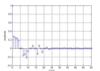
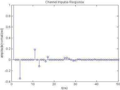
(13) State 1:. u1 e − u1k . k!. (2.1). u 2 e − u2 k P (nl = k ) = . k!. (2.2). P (nl = k ) =. k. State 2: k. In the above equations, u1 = ∫ λ1 (t )dt and u2 = ∫ λ2 (t )dt are the Poisson parameters; Tc. Tc. λ1 (t ) and λ2 (t ) are the mean number of paths arriving at time t. State 1 denotes the state that arises when no paths are present in the previous time bin, and state 2 reprents the opposite case when paths are present in the previous time bin. Also, a Gamma distribution is employed to demonstrate the power distribution. In this thesis, we will focus on the light-of-sight (LOS) situation. Hence, the first multipath component will be multiplied by the LOS power-gain factor equal to 5dB relative to the second multipath component. Fig. 2.1 shows the simulation of this channel model with 50 multipaths and a time bin of 1ns. It is found that most of the conspicuous multipath components are presented within t < 25ns.. 8.

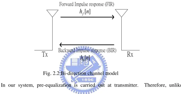
(14) Fig. 2.1 Simulation result of the multipath channel.. 2.2 System Model Using discrete-time signal representation, if a slow fading channel is assumed, it can be modeled as below [9].. N. h[n ] = ∑ α l e jθl δ [n − l ],. (2.3). l =0. where α l. and θ l. are the relative fading amplitude and cumulative phase. corresponding to the lth path. Fig. 2.2 illustrates a bi-direction channel model, where. h f [n ] and hb [n ] specify the forward impulse response (FIR) and the backward impulse response (BIR), respectively. In our system, we consider bipolar pulses so that. θ l in (2.3) will be simplified to 0 or π . The FIR and the BIR can be given respectively as Nf. h f [n] = ∑ α l δ [ n − l ] , l =0. 9. (2.4).

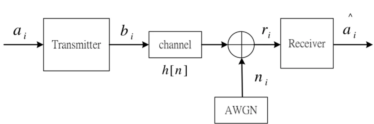
(15) Nb. hb [n] = ∑ β l δ [n − l ] .. (2.5). l =0. where α l and β l are the relative amplitudes at the lth path of FIR and BIR, while N f and N b are the numbers of FIR and BIR multipath components. Here, we assume. N f = N b = N =50 to simplify the follow analysis.. h f [n]. hb[n] Fig. 2.2 Bi-direction channel model In our system, pre-equalization is carried out at transmitter.. Therefore, unlike. traditional ISI management, the FIR of the channel should be known in advance. Then, the distortion caused by multipath can be measured subsequently. Due to the reciprocity property of TX/RX antennas, FIR and BIR of the channel are symmetric. Consequently, (2.4) and (2.5) can be simplified as. N. h f [n ] = hb [n ] = h[n ] = ∑ α l δ [n − l ] .. (2.6). l =0. Figure 2.3 illustrates the wireless transmission model over a channel with intersymbol interference and additive Gaussian noise. In this figure, a i is the discrete-time data, bi is the modified data signal, and h[n ] is the channel impulse 10.

(16) response with intersymbol interference as described in (2.6). The Fourier transform of. h[n ] is H ( f ) . ^. ai. ri. bi h [n ]. ai. ni. Fig. 2.3 Wireless transmission model. If we assume that h[n ] is normalized so that α 0 = 1 , then the channel output is given by N. N. k =0. k =1. ri = ∑α k bi −k + ni =bi + ∑α k bi −k + ni ,. (2.7). where ni is the additive noise, which is assumed to be statistically independent of bi . The second term in (2.7), that is N. Ψi = ∑ α k bi −k ,. (2.8). k =1. is corresponding to the intersymbol interference, being determined by previous modified data d k −l ' . If we choose the modified data as. bi = a i − Ψi .. The following equation is obtained from (2.7) and (2.9). 11. (2.9).

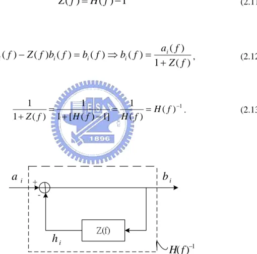
(17) ri = ai + ni .. (2.10). It shows that the received signal rk would only be interfered by the additive noise. A circuit implemented corresponding to (2.9) is shown in Fig. 2.4, where the transfer function of the feedback filter is given by. Z ( f ) = H ( f ) −1. (2.11). In this case,. ai ( f ) − Z ( f )bi ( f ) = bi ( f ) ⇒ bi ( f ) =. ai ( f ) , 1+ Z( f ). 1 1 1 = = = H ( f ) −1 . 1 + Z ( f ) 1 + [ H ( f ) − 1] H ( f ). ai. (2.12). (2.13). bi. hi. H( f )−1. Fig. 2.4 Block diagram of transmitter in pre-equalization technique. It means that we can move the linear equalization from receiver to transmitter. Namely, we can solve the intersymbol interference problem directly at TX with pre-equalization filteing. A circuit named the multipath processor (MP) is designed at transmitter to implement 12.

(18) the inverse filter H ( f ) −1 and to measure the channel coefficients. The circuit diagram of MP is shown in Fig. 2.5, being an IIR filter-like structure. Its input/output relationship is written as. L. y[n] = p0 ⋅ ( x[n] − ∑ pl y[n − l ]) .. (2.14). l =1. where L is the number of taps in the MP.. x[n]. y[n]. p0. Z-1 p1. Z-1 p2. Z-1 pL-1. Z-1 pL. Fig. 2.5 The multipath processor for registering the multipath coefficients. In the ideal measuring process without channel noise, the receiver sends an impulse to the transmitter and all the channel components will be registered accurately. Then the MP applies the channel components ( α l , l=0,1,2…,N) to specify its tap coefficients as. p0 = 1 / α 0 = 1 ,. (2.15). pl = α l , l=1,2,…,N.. (2.16). 13.

(19) 2.3 System Description 2.3.1 System Design Concept While a series of data stream D[n ] = ∑ d k δ [n − k ] , d k ∈ {1,−1} , is sent to the RX k. via a noiseless multipath channel, the received signal is written as. N. R[n ] = D[n ] ⊗ h f [n ] = D[n ] ⊗ ∑ α l δ [n − l ].. (2.17). l =0. At some time instant, the received signal can be represented as. R[n] = rk ⋅ δ [n − k ] , rk = α 0 d k + ∑α l d k −l = α 0 d k + Ψk .. (2.18) (2.19). l. where Ψk corresponds to the multipath-induced ISI resulted from the previous data. Since Ψk is a random variable depending on the multipath coefficients and the polarity of past data, it will lead to performance degradation. In the proposed system, the multipath coefficients can be accurately measured at TX according to the measuring process described in Section 2.2. Using the measured multipath coefficients, we can pre-determine the amount of multipath-induced ISI before d k is sent and appropriately modify the amplitude of d k . Let d k' denote the modified signal amplitude. Replacing d k with d k' , then (2.19) is reformulated as. rk = α 0 d k' + ∑ α l d k' −l = α 0 d k' + Ψk , l. 14. (2.20).

(20) Ψk = ∑ α l d k' −l ,. (2.21). l. where Ψk. is again the amount of multipath-induced ISI produced by the past data. We. can modify the MP of Fig. 2.3 to estimate Ψk at TX. Fig. 2.6 demonstrates the circuit of the modified MP.. Fig. 2.6 The modified MP for estimating the amount of Ψ. Assuming the FIR coefficients are accurately measured, the tap coefficients of the modified MP are specified as. pl = α l , l = 1,2,...N .. Thus the value of Ψk can be exactly estimated.. 15. (2.22).

(21) 2.3.2 Determination of the Modified Data d k' 2.3.2.1 One Bit Pre-Equalization with Stable Channel Coefficients Because MP is an IIR-filter like structure, channel coefficients should be checked if the filter is stable or not. An IIR filter could be characterized by the transfer function as. H ( z) =. Q ( z ) q0 + q1 z −1 + L + qn z − n = D( z ) 1 + d1 z −1 + L + d n z −n. (2.23). So the transfer function of MP can be characterized as. H ( z) =. 1 1 = . −1 D ( z ) 1 + α1 z + L + α n z −n. (2.24). where q0 = 1 , q1 = q2 = L = qn = 0 , and d n = α n , n = 1,2, L , N . Therefore we could plot the zero-pole diagram to check if the poles are located inside or outside the unit circle. When the channel is stable, d k' could be convergent. If we let rk be designed to have the same polarity as d k and be equal to a specific threshold so as to combat the channel noise. Then, the following equality holds for rk :. rk ⋅ d k = ξ ,. (2.25). where ξ is the threshold and is a positive number. From (2.19), we have. α 0 d k ' d k + Ψk d k = ξ .. 16. (2.26).

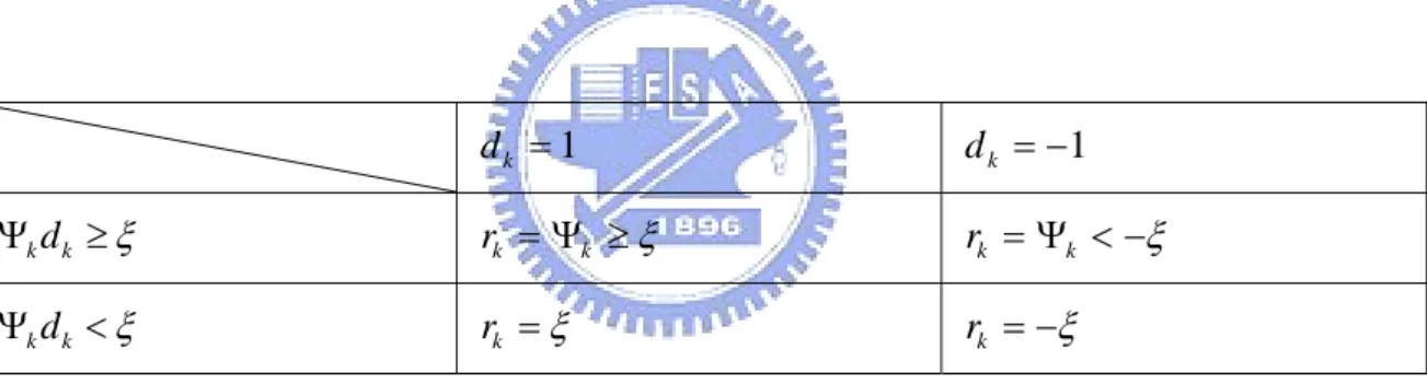
(22) Then,. dk ' =. ξ − d k Ψk , α 0d k. (2.27). Assume the multipath component Ψk be measured correctly, from (2.27), the modified data d k' would let the received data rk =. ξ dk. rk = α 0 d k '+ Ψk = α 0. . In this case,. ξ − d kψ k ξ +ψ k = . α 0d k dk. (2.28). And the decision of rk would be only distorted by the additional noise. Nevertheless, if channel is unstable, d k' could be divergent.. 2.3.2.2 One Bit Pre-Equalization with Unstable Channel Coefficients In the previous section, we mention that if the channel is unstable, d k' could diverge toward infinity. Under this condition, we develop a solution to deal with the problem. Let rk be designed to have the same polarity as d k and its magnitude equal to or exceed a specific threshold so as to combat the channel noise. Then, the following inequality holds for rk :. rk ⋅ d k ≥ ξ ,. (2.29). where ξ is the threshold and is a positive number. From (2.20), we have. α 0 d k ' d k + Ψk d k ≥ ξ .. 17. (2.30).

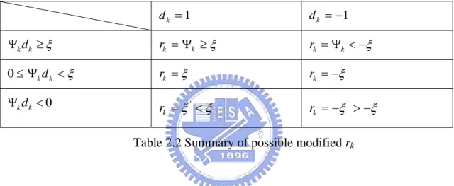
(23) If Ψk d k ≥ ξ , which means that the magnitude of Ψk d k is larger than ξ . In such a condition, the best choice is d k' = 0 to save transmission power. Namely, the system is in the idle state without sending any signal and rk = Ψk . Next, if Ψk d k < ξ , according to (2.30), we obtain α 0 d k' d k ≥ ξ - Ψk d k . The equality holds, if we choose d k' as. d k' =. In this case, rk = α 0 d k' + Ψk =. ξ dk. ξ - Ψk d k α 0d k. .. (2.31). = d k ξ . Table 2.1 summarizes the four possible rk. due to different multipath conditions and polarities of data.. dk = 1. d k = −1. Ψk d k ≥ ξ. rk = Ψk ≥ ξ. rk = Ψk < −ξ. Ψk d k < ξ. rk = ξ. rk = −ξ. Table 2.1 Summary of possible rk. If we focus on the theme of saving transmitted power, from (2.30) there is another variable we could consider, i.e. the threshold ξ . Eq. (2.30) could be rewritten as. α 0 d k'' d k + Ψk d k ≥ ξ ' ,. (2.32). If Ψk d k < 0 , that means ISI caused by multipath has different polarity as the input data. Therefore, the modified data d k'' would need addition amplitude to counteract the ISI for meeting the threshold. Under this conditon, we could lower the threshold to save power. 18.

(24) The equality holds if d k'' is chosen as. ξ ' - Ψk d k d = α 0d k '' k. .. (2.33). Table 2.1 could be renewed to summarize the six possible rk as shown in Table 2.2. From Table 2.2, the first two conditions have the same property. Because ISI induced by multipath has the same polarity as the input data, it can be used directly as the transmitted signal. However, the last two conditions are contrary as the first two.. dk = 1. d k = −1. Ψk d k ≥ ξ. rk = Ψk ≥ ξ. rk = Ψk < −ξ. 0 ≤ Ψk d k < ξ. rk = ξ. rk = −ξ. Ψk d k < 0. rk = ξ ' < ξ. rk = −ξ ' > −ξ. Table 2.2 Summary of possible modified rk. 2.3.2.3 Two-Bits Pre-Equalization with Unstable Channel Coefficients As described in the previous section, we consider the effect of multipath imposed on the upcoming data. We utilize it to help transmission and to save transmission power. But there is another information we did not think of. At TX, we could not only obtain the multipath component, but also have the information of the upcoming data. In this section, we would take this advantage and exploit what we can do to improve system performance. Under the condition that the channel is line-of-sight (LOS) and normalized, the maximum channel coefficient except the first one is found out first. Similar to (2.18)-(2.20), at some time instant, the anticipated received signal can be represented as. R[n] = rk ⋅ δ [ n − k ] , 19. (2.34).

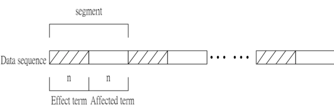
(25) rk = α 0 d k '+ ∑α l d k −l ' = α 0 d k '+ Ψk .. (2.35). l. Thus, N. rk +n = α 0 d k +n '+ L + α n d k '+ ∑α l d k +n −l = α 0 d k +n '+ L + α n d k '+ Ψk +n ,. (2.36). l = n +1. where α n is the maximum channel coefficient except the first one. From (2.35) and (2.36), it shows that the modified data d k ' would be the dominate term on determining d k + n ' . From (2.36), rk + n +1 , rk + n + 2 ,LL, rk + 2 n −1 can be written as. rk +n+1 = α 0 d k +n+1 '+ L + α n d k +1 '+ Ψk +n+1 ,. (2.37). rk + n + 2 = α 0 d k +n +2 '+L + α n d k + 2 '+ Ψk +n +2 ,. (2.38). M M. rk + 2 n −1 = α 0 d k +2 n −1 '+L + α n d k +n −1 '+ Ψk +2 n −1 .. (2.39). Therefore, from (2.37)-(2.39), it can be shown that d k +1 ' would affect d k + n +1 ' mostly, d k + 2 ' would seriously affect d k + n + 2 ' and so on. At last, d k + n −1 ' would affect d k + 2 n −1 ' mostly. We take 2n bits as a segment to find out the new management rule. It can be found that the former n bits could be considered as the effect terms; while the latter n bits are affected terms. Figure 2.7 illustrates the data sequences being partitioned into many segments. In each segment, ISI introduced by the effect terms would be considered if it is constructive or destructive to the affected terms in advance.. 20.

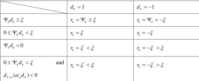
(26) LL Fig. 2.7 Segmented data sequences. Apply the same criterion as shown in (2.30), (2.35) and (2.36) could be rewritten as. d k rk = d k (α 0 d k '+ ∑α l d k −l ') = d k α 0 d k '+ d k Ψk ≥ ξ ,. (2.40). l. d k + n rk + n = α 0 d k + n ' d k + n + L + α n d k ' d k + n + Ψk + n d k + n ≥ ξ .. (2.41). While determining d k ' , we should considered not only the interference caused by previous data, but also the interference induced by d k ' to the next n-th data. Besides the decision rule shown in Table 2.2, there is another condition that the threshold ξ should be adjusted. If d k + n (α n d k ) < 0 , meaning that intersymbol interference caused by d k is destructive, the threshold in (2.40) will be lowered for saving transmission power and decreasing the ISI distortion. Therefore, Table 2.2 should be modified. Table 2.3 shows the possible rk under four conditions.. 21.

(27) dk = 1. d k = −1. Ψk d k ≥ ξ. rk = Ψk ≥ ξ. rk = Ψk < −ξ. 0 ≤ Ψk d k < ξ. rk = ξ. rk = −ξ. Ψk d k < 0. rk = ξ ' < ξ. rk = −ξ ' > ξ. rk = ξ ' < ξ. rk = −ξ ' > ξ. 0 ≤ Ψk d k < ξ. and. d k + n (α n d k ) < 0 Table 2.3 Possible rk under two-bit consideration. 22.

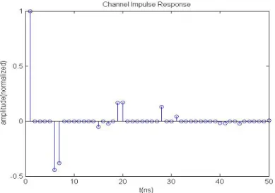
(28) Chapter 3 Performance Analysis. 3.1 System Performance. dk. dk '. MP. rk. channel. h [n ]. detector. decision. ni. Ψk. AWGN. Fig. 3.1 Transmission model. Figure 3.1 illustrates the transmission model we will use in the following simulation, where d k is the transmitted data, d k' is the modified data signal and rk is the received signal. In this model, the receiver is very simple, only the detector and the decision function are needed. We let d k = 1 so that the average power of data is 1. In order to compare the performance under different channel conditions, we adopt three channel coefficients as shown in Figs. (3.2)-(3.4). Figure 3.2 Channel impulse response A 23.

(29) Figure 3.3 Channel impulse response B. Figure 3.4 Channel impulse response C. In these fading channels, it can be shown that the number of multipath is channel A < channel B < channel C. Fig. 3.5 provides the BER corresponding to three channels with different received SNR under ideal transmission condition. In ideal transmission condition, the multipath coefficients are assumed to be measured without noise, so the corresponding Ψk can be accurately obtained.. 24.

(30) Figure 3.5 Performance of proposed system. In Fig. 3.5, the thick solid line is the BER of the bipolar data passing through a multipath-free channel, being interfered only by the additive Gaussian noise. The circle line corresponds to direct transmission without any ISI management, where performance is quite poor compared to the multipath-free channel. It is shown that the ISI significantly degrades system performance. Both conditions will be used as the reference for comparison. In order to compare with the case of multipath-free transmission, we define the received SNR as. SNRr = 10 log(. Pr ), N 0 ⋅ BW. (3.1). where Pr is the average power of rk , BW is the bandwidth and N 0 is the noise power spectral density. In Fig. 3.5, it is shown that the BER performance of channel-A shown in Fig. 3.2 is the best. It approaches the case of multipath-free transmission. From Table 2.1, it implies that the magnitude of rk will be equal to the specified threshold without the idle state.. 25.

(31) While ξ = 1 , there are 97.52% of rk equal to 1 in the simulation. If the idle state occurs, the induced-ISI directly serves as rk , the magnitude will be larger than the threshold. Moreover, Pr is 1.008512 which is a little larger than 1. We record the related percentage of idle state and the received power of the simulated channel in Table 3.1.. average received channel. idle state(%) power. Channel A. 2.48. 1.008512. Channel B. 16.21. 1.266794. Channel C. 22.49. 1.677684. Table 3.1 Idle state and received power in fig. 3.5. We find that the more multiapth components, the larger percentage of the idle state as well as the average received power. Therefore, the BER for a fixed SNR is channel A < channel B < channel C.. 3.2 Analysis of System Characteristics In the previous section, we assumed that simulation is under ideal transmission. Also, in Fig. 3.2 - 3.4, mulipath coefficients mostly appear within t=30ns. In reality, the proposed system will not be able to achieve the multipath-free transmission because the system complexity would limit the number of taps in the MP. Hence, we can only obtain the essential portion of the channel multipath coefficients instead of getting all of them. Thus some tap length of MP would be sufficient to simplify the transmitter complexity. We perform computer simulation for three different channels to find sufficient tap numbers. In each simulation, the threshold is equal to 1.. 26.

(32) Figure 3.6 BER vs. SNRr for different MP tap lengths under channel A. Fig. 3.6 depicts the BER according to different tap length of the modified MP for channel A. For L=10, the tap number is insufficient, since the performance significantly deviated from the case of multipath-free transmission. This is because there are still many multipath coefficients between L=10 and L=20. However, while L>20, as sufficient taps are included, the performance approaches to the multipath-free transmission.. Figure 3.7 BER vs. SNRr for different MP tap lengths under channel B. 27.

(33) In the case of channel B as depicted in Fig. 3.7, while L=10, the BER performs badly. It is because the tap number is not sufficient so that ISI caused by multipath can not be eliminated efficiently. When L>20, the performance is better as L becomes large. From Fig. 3.3, it can be shown that most multipath coefficients occur before t<30ns. Hence, while L=30, the BER performance is the almost the same as L=50.. Figure 3.8 BER vs. SNRr for different MP tap lengths under channel C. Because the multipath coefficients of channel C occur before t<30ns, Fig. 3.8 shows similarly result as Fig. 3.7. But the number of multipath components shown in channel B is less than that in channel C, the BER performance of Fig. 3.8 is thus worse than Fig. 3.7.. 3.3 Adjustment of Threshold After clarifying the system capability and characteristics, we proceed to discuss the properties of average transmitted and received power which are the average power of d k' and rk , respectively. In the following simulation, we let rk = ±1 and change the 28.

(34) threshold ξ discussed in table 2.1. We illustrate the average power of d k' in Fig. 3.9.. Figure 3.9 The simulated average transmitted power under these three channels. Fig. 3.9 indicates the tendency that the average transmitted power increases as the threshold getting larger. However, if a channel has few multipath components like channel A, the change of average transmitted power is little. It is because the estimated ISI is not big enough to exceed the threshold. However, if a channel has a large number of multipath components like channel B or channel C, the change of the average transmitted power is significant. In these cases, the estimated ISI would be much bigger. While the threshold is increased, it means that the transmitter is willing to spend more transmitted power to let rk equal to 1. Therefore, it is expected that BER performance would become better as the threshold getting larger. Table 3.2 records the percentage of idle state.. 29.

(35) idle state (%). idle state (%) idle state (%). (channel A). (channel B). threshold (channel C). 0.2. 37.15. 41.97. 43.83. 0.4. 24.89. 34.61. 37.98. 0.6. 14.05. 27.75. 32.39. 0.8. 6.57. 21.52. 27.15. 1. 2.48. 16.22. 22.47. 2. 0. 3.29. 8.59. 3. 0. 0.5. 3.91. 4. 0. 0.038. 2.12. 5. 0. 0.001. 1.29. 6. 0. 0. 0.81. Table 3.2 The simulated percentage of idle state. Table 3.2 demonstrates that the percentage of idle state decreases as the threshold increases. It is because if the threshold is large, the estimated ISI has less chance to satisfy d k Ψ k ≥ ξ . Figs. 3.9, 3.10 and 3.11 provide the BER performance of the cases with the threshold bigger and smaller than 1 for channel B, respectively. In Fig 3.10, the BER becomes smaller with higher ξ , but more transmission power is needed. According to Table 3.2, if the threshold increases, the percentage of idle state decreases. From Table 2.1, if the percentage of idle state decreases, the probability of d k ' = 0 also decreases. This means more transmitted power is necessary to let the received power equal 1. Hence, the average transmitted power will increase if the. 30.

(36) threshold increases. According to (3.1), under the same SNR, if p r is small, N 0 will be small, too. Therefore, decision of received data would be affected less by noise as the threshold increases. So BER should be improved while ξ is getting larger. Intuitively, we could adjust the threshold to transmit acceptable power to achieve a better BER. Table 3.3 records the related average transmitted power.. Fig 3.10 BER vs. received SNR for judged threshold larger than 1. average threshold transmitted power 1. 1.9682. 2. 2.0977. 3. 2.3528. 4. 2.4961. 5. 2.5321. 6. 2.5336. Table 3.3 The simulated average transmitted power of judged threshold larger than 1 31.

(37) In Fig. 3.11, the BER becomes worse with smaller ξ , but transmitted power decreases accordingly. From Table 3.2, while the threshold decreases, the occurrence of idle states will increase. Hence, the percentage of rk = Ψk and d k ' = 0 will increase, too. Since ξ is small, Ψk is small as well, and rk = Ψk would be sensitive to the noise. Therefore, BER would be worse while the threshold is low. However, although the percentage of d k ' = 0 increases, the average transmitted power is slightly decreased. From Table 3.2, the occurrence of idle state increases while the threshold deceases, it also means that the percentage of d k ' = 0 increases. This result should lower the average transmitted power. However, if ISI induced by d k ' before lowering the threshold is constructive to some upcoming data d k +n , the modified data d k ' = 0 after lowering the threshold would lead d k +n transmit more power to compensate the ISI induced by d k ' . Therefore, because of the offset between these two results, the amount of the saved transmitted power is slightly. Table 3.4 records the simulated average transmitted power for different thresholds.. Fig. 3.11 BER vs. received SNR for judged threshold smaller than 1. 32.

(38) average threshold transmitted power 1. 1.969. 0.8. 1.971. 0.6. 1.973. 0.4. 1.957. 0.2. 1.892. Table 3.4 The simulated average transmitted power of judged threshold smaller than 1. 3.4 Power Saving for One-Bit System In the previous section, transmitted power decreases while lowering the threshold. However, BER would be much worse. If we do not adjust the threshold while ISI and the current data have different polarity, the transmitter should spend more power to let the received amplitude equal to the threshold. Therefore, if ISI is destructive to the current data, we could lower the threshold to save power. That is, we would allow the received amplitude under the threshold. In this simulation, we let ξ = 1 and adjust ξ ' in Table 2.2 to see the change of BER and the average transmitted power. Fig 3.12 represents the BER according to different thresholds. Table 3.5 records the related average transmitted power.. 33.

(39) Fig. 3.12 BER vs. received SNR for modified threshold smaller than 1. average threshold transmitted power 1. 1.9679. 0.9. 1.6422. 0.8. 1.3571. 0.7. 1.1102. 0.6. 0.9029. 0.5. 0.7326. Table 3.5 The simulated average transmitted power of modified threshold smaller than 1. In Fig. 3.12 and Table 3.5, it can be shown that BER would be worse as the threshold getting smaller, and the related average transmitted power would decrease. If the threshold decreases, from Table 2.2, the amplitude of received data rk = ξ ' will. be. reduced. Therefore, the received data would be more sensitive to noise. Hence, BER 34.

(40) would get worse as the threshold decreases. On the other hand, the average transmitted power decreases obviously as the threshold decreases. That is because we only lower the transmitted power while ISI is destructive to the upcoming data, the average transmitted power would decrease while the threshold decreases.. 3.5 Analysis of Power Saving for Two-Bit System After clarifying the case of modifying the threshold in one-bit system, we now consider two-bit system. In Chapter 2.3.2.3, we explained that there was another information we can obtain at transmitter, which is the content of upcoming data. Therefore, as channel coefficients are accurately measured in advance, we could find out which subsequent data would be affected mostly by the current data. And then, ISI induced by the current data would be checked if it is helpful to this mostly-affected data. If it is not, we will reduce the threshold as the same setup of one-bit system to save power. Fig 3.13 depicts the BER performance of different threshold and the comparison of one-bit and two-bit systems. Table 3.6 records the simulated average transmitted power and compare with one-bit system.. Fig 3.13 Comparison of one bit and two bits BER vs. received SNR 35.

(41) average. average. transmitted transmitted threshold power. power. (one bit). (two bit). 1. 1.968. 1.968. 0.9. 1.642. 1.615. 0.8. 1.357. 1.306. 0.7. 1.11. 1.039. 0.6. 0.903. 0.82. 0.5. 0.733. 0.645. Table 3.6 The simulated average transmitted power under one-bit and two-bit systems. In Fig. 3.13, BER performance for two-bit system is close to that of one-bit system. However, the BER of two-bit system is a little better than one-bit system. It is because the ISI effect of the proceeding data is reduced in advance. Also, besides modifying threshold while ISI effect is destructive to the current data, the threshold is also modified. Therefore, average transmitted power is saved as comparing with one-bit system.. 36.

(42) Chapter 4 Conclusions This thesis presents a transmission scheme to solve the ISI problem while transmit speed raises to Gbps. This method utilizes measured channel coefficients to manage multipath-induced ISI and set the amplitude of noiseless received signal. The proposed system structure moves the equalization functionality to the transmitting end. The developed MP circuit at TX can first measure the channel response coefficients. Next, the modified MP can estimate the related ISI effect. According to the estimated ISI, the threshold mechanism is excuted to determine the amplitude of transmitted signal. After transmitting these signals through the multipath channel, the related output signal will be defined by a threshold. While the threshold equals to the data magnitude, the BER performance can approach the ideal multipath-free transmission. The BER could be improved by transmitting more power. The transmitted power could be reduced by lowering the threshold while ISI and the current data have different polarity. While the channel SNR is high, we can choose small threshold so as to save power but still maintain acceptable BER. At last, a two-bit system is proposed to improve BER performance and save transmitted power. Although its improvement is not obvious, it could be a useful system for future study.. 37.

(43) Reference [1] “FCC notice of proposed rule making, revision of part 15 of the commission’s rules regarding. ultra-wideband. transmission. systems,”. Federal. Communications. Commission, Washington, DC, ET-Docket 98-153. [2] S. Roy, J. R. Foerster, V. S. Somayazulu, and D. G. Leeper, “Ultrawideband Radio Design: The Promise of High-Speed, Short-Rang Wireless Connectivity,” Proc. of the IEEE, Vol.92, No.2, Feb. 2004, pp.259-311 [3] R.. C.. Qui,. H.. Liu,. X.. Shen,. “Ultra-Wideband. for. Multiple. Access. Communications,” IEEE Communications Magazine, Feb. 2005. [4] J. D. Choi and W. E. Stark, “Performance of Ultra-Wideband Communications with Suboptimal Receiver in Multipath Channels,” IEEE Journal on Selected Areas in Communications, Vol.20, No.9, Dec. 2002, pp.1754-1766 [5] R. Hoctor, H. Tomlinson, “An overview of Delay-Hopped Transmitted-Reference RF Communications,” IEEE Conf. on Ultra Wideband Syetem and Technologies, May 2002, pp. 265-269 [6] M. Ho, V. S. Somayazulu, J. Foerster, S. Roy, “A Differential Detector for an Ultra-Wideband Communication System,” IEEE Vehicular Technology Conference, May 2002, vol.4, pp.1896-1900 [7] S. Zhao, H. Liu, and Z. Tian, “A Decision-Feedback Autocorrelation Receiver for Pulsed Ultra-Wideband Systems,” IEEE Radio and Wireless Conference, Sept. 2004, pp. 251-254 [8] S. M. Emami et al.,“Predicted Time Reversal Performance in Wireless Communications Using Channel Measurements,” to appear in IEEE Communication Lett.. 38.

(44) [9] Harashima H. and Miyakawa H., “Matched-Transmission Technique for Channels With Intersymbol Interference,” Communications, IEEE Transactions on legacy, pre- 1988 [10] A. Lender, “Correlative digital communication techniques,” IEEE Trans. Commun. Technol. Vol. COM-12, pp. 128-135 Dec. 1964. [11] E. R. Kretzmer, “Generalization of a technique for binary data communication,” IEEE Trans. Commun. Technol. (Concise papers), vol. COM-14, pp. 67-68, Feb. 1996. [12] F. Zhu, Z. Wu, and C. R. Nassar, “Generalized Fading Channel Model with Application to UWB,” IEEE Conf. on Ultra Wideband Syetem and Technologies, May 2002, pp.13-17. 39.

(45) 簡. 姓. 歷. 名：陳柏任. 居住地：台灣省台北縣出生年月：民國七十年七月十一日學經歷：國立交通大學電信工程學系. (88 年 9 月~ 92 年 6 月). 國立交通大學電信工程學系碩士班. (93 年 9 月~ 96 年 2 月). 40.

(46)