光學玻璃透鏡熱壓成形之模具最佳化設計

全文

(1)國立交通大學機械工程學系碩士論文. 光學玻璃透鏡熱壓成形之模具最佳化設計 Die Shape Optimization on Molding Process of Optical Glass Lens. 研究生：吳宗駿指導教授：洪景華教授. 中華民國九十六年六月.

(2) 光學玻璃透鏡熱壓成形之模具最佳化設計 Die Shape Optimization on Molding Process of Optical Glass Lens 研. 究. 生：吳宗駿. Student： Tsung-Chun Wu. 指導教授：洪景華教授. Advisor： Dr. Chinghua Hung. 國立交通大學機械工程學系碩士論文. A Thesis Submitted to Department of Mechanical Engineering College of Engineering National Chiao Tung University in Partial Fulfillment of the Requirements for the Degree of Master in Mechanical Engineering. June 2007 Hsinchu, Taiwan, Republic of China 中華民國九十六年六月.

(3) 光學玻璃透鏡熱壓成形之模具最佳化設計. 學生：吳宗駿. 指導教授：洪景華教授. 國立交通大學機械工程學系摘要. 光學玻璃透鏡的需求隨著光電科技產品的發展而日益增加。對於光學玻璃材料而言，熱壓成形技術相對於傳統的研磨拋光技術，擁有許多優勢，可達成節省成本且量產的目的。然而，光學玻璃透鏡熱壓成形仍然有許多必須克服的難題，如玻璃透鏡成品的尺寸誤差會影響鏡片的成像品質等等。本論文主要分成兩個部分，第一部份為利用有限元素分析軟體，以熱偶合分析的方式模擬玻璃透鏡熱壓的過程。第二部份則建立一模具補償的最佳化系統，自動化連結有限元素分析軟體與最佳化程式。利用有限元素分析的結果，作為最佳化設計的條件，其中以原始設計尺寸與玻璃透鏡成品之間誤差的均方根值為目標函數，期望能有效的減少誤差的比率，提高透鏡成品的品質。. I.

(4) Die Shape Optimization on Molding Process of Optical Glass Lens Student：Tsung-Chun Wu. Advisor：Dr. Chinghua Hung. National Chiao Tung University Department of Mechanical Engineering. Abstract Demand of optical glass lens is progressively increasing with the development of optical and electrical products. As far as the optical glass material is concerned, lens molding technique, compared with the conventional glass lens grinding and polishing process, has lots of advantages, like much simplified manufacture process and dramatically reduction of cost and waste. However, there still exist several difficulties needed to be overcome, such as the shape deviations of the final lens products that may influence the qualities of optical image. This thesis is primarily divided into two parts. The first one is to simulate the glass lens molding process using thermal-mechanical coupled analysis with the finite element method. The second part is to construct a die shape optimization system in order to compensate automatically for the shape deviations of the lens products so that the errors can be reduced efficiently. Once the deviations of the lens products have been minimized, the aim of mass production for lens molding of optical glass can be accomplished.. II.

(5) 誌謝走在待了六年的交大校園裡，感受烈日與暖風，才發覺離情依依的畢業季節又悄悄地來到。隨著夏日溫度的增加，完成學業的喜悅與離開熟悉環境的感傷也在我的心中逐漸地蔓延擴散。在過去兩年的研究所碩士生涯裡，首先，我要感謝的人是我的指導教授洪景華老師，在學業上與研究中所提供的教導與意見，都使我獲益良多。同時也感謝口試委員陳復國教授、賀陳弘教授、徐瑞坤教授，對於論文所提出的指正與建議。其次，感謝精密工程與模擬實驗室的所有成員，已經畢業的洪榮崇學長，告訴我許多玻璃模造知識的宇中學長、嘉偉學長，感謝你們的協助，讓我得以順利完成這篇論文。還有政成學長、煌棊學長、正展學長、銘傑學長、麒禎學長，感謝你們在課業上的幫忙與意見。感謝兩年來一起同甘共苦的同學小強、彥彬和黃詠，還有世璿、志嘉、運賢與俊羿學弟。感謝實驗室的大家，和你們一起生活的兩年，帶給我充滿歡笑與快樂的回憶。此外，我要特別感謝我的父親、母親、妹妹，在我求學的過程中給我的支持與鼓勵，讓我沒有後顧之憂，可以專心在學業上面，謝謝你們。最後，我想以“Where there is a will, there is a way.＂與大家共勉。希望大家都能堅持自己的初衷、理想與夢想，繼續加油下去，往目標邁進。感謝這一路上所有曾經陪伴過我、幫助過我的人。謝謝你們！. III.

(6) Table of Contents 摘要............................................................................................................. I Abstract ......................................................................................................II 誌謝...........................................................................................................III Table of Contents ..................................................................................... IV List of Figures .......................................................................................... VI List of Tables............................................................................................ IX Chapter 1 Introduction ................................................................................1 1.1 Optical Lenses.......................................................................1 1.2 Lens Molding of Optical Glass.............................................2 1.3 Literature Review .................................................................4 1.4 Motivation and Objectives....................................................5 1.5 Research Method ..................................................................6 1.6 Thesis Outlines .....................................................................7 Chapter 2 Optical Glass Material .............................................................10 2.1 Characteristic of Glasses.....................................................10 2.2 Classifications of Optical Glasses ......................................10 2.3 Material Properties of Optical Glasses ...............................11 2.3.1 Optical Properties ......................................................11 2.3.2 Mechanical Properties ...............................................13 2.3.3 Thermal Properties.....................................................15 2.3.4 Other Properties .........................................................16 Chapter 3 Finite Element Analysis ...........................................................20 3.1 Introduction of FEA............................................................20 3.2 FEA Software......................................................................20 3.3 Process of Glass Lens Molding ..........................................21 IV.

(7) 3.4 Finite Element Analysis......................................................22 3.4.1 Geometrical Model ....................................................22 3.4.2 Material Properties.....................................................23 3.4.3 Boundary Conditions .................................................25 3.4.4 Contact Surfaces ........................................................26 3.4.5 Mesh Density Tests....................................................26 3.5 Results and Discussions......................................................27 Chapter 4 Die Shape Optimization ...........................................................44 4.1 Introduction.........................................................................44 4.2 Fundamental Theory of Optimization ................................45 4.3 The Optimization Algorithm...............................................47 4.4 Optimization Implement.....................................................47 4.5 Integration of FEA and Optimization .................................48 4.6 Formulation of Optimization System .................................48 4.6.1 Design Variables ........................................................48 4.6.2 Objective Function.....................................................50 4.6.3 Constraints .................................................................50 4.7 Results and Discussions......................................................51 Chapter 5 Conclusions and Future Works ................................................75 5.1 Conclusions.........................................................................75 5.2 Future Works.......................................................................76 References.................................................................................................78 Appendix A Uniaxial Compression Experiments..................................80 A.1 Experiments: ......................................................................80 A.2 Related Simulations: ..........................................................80 A.3 Results and Discussions.....................................................81 Appendix B. Linking Program Code ......................................................85. Appendix C. User’s Subroutine Code ....................................................91 V.

(8) List of Figures Figure 1.1 Open-die molding process of optical glass lens........................9 Figure 2.1 Specific volume variation with temperature ...........................18 Figure 2.2 nd–νd diagram of optical glasses for glass mold optics [7]......19 Figure 3.1 Temperature history diagram...................................................30 Figure 3.2 Geometrical model in detailed size of both dies and glass. (Unit : mm) ...................................................................................................31 Figure 3.3 Relations between stress and strain with different strain rate at 475℃.................................................................................................32 Figure 3.4 Young’s modulus as a function of the temperature. ...............32 Figure 3.5 Boundary conditions in axisymmetric analysis model ...........33 Figure 3.6 Points for conducting the mesh density tests. .........................34 Figure 3.7 Convergence of axial displacement at point A........................35 Figure 3.8 Convergence of von Mises stress at point B. ..........................35 Figure 3.9 Simulated process of lens molding. ........................................36 Figure 3.10 Axial displacement of glass formed lens...............................37 Figure 3.11 Radial displacement of glass formed lens(at 475℃). ...........38 Figure 3.12 von Mises Stress distribution of formed lens during cooling VI.

(9) cycle. .................................................................................................39 Figure 3.13 (continued) von Mises Stress distribution of formed lens during cooling cycle..........................................................................40 Figure 3.14 Die shape deviation due to thermal expansion......................41 Figure 3.15 Geometrical err of lens curve after cooling stage .................42 Figure 3.16 Comparison between the designed and formed lens curve. ..43 Figure 3.17 Error between the designed and formed lens. .......................43 Figure 4.1 Procedure of optimum design [12]..........................................57 Figure 4.2 Integration procedure of FEA and optimization .....................58 Figure 4.3 Design variables in optimization procedure............................59 Figure 4.4 Conic section curves................................................................60 Figure 4.5 Die shape curve with R =10mm (spherical)............................61 Figure 4.6 Glass formed lens curve with R =10mm (spherical)...............61 Figure 4.7 Die shape curve with R =10mm (parabolic) ...........................62 Figure 4.8 Glass formed lens curve with R =10mm (parabolic) ..............62 Figure 4.9 Die shape curve with R =10mm (hyperbolic) .........................63 Figure 4.10 Glass formed lens curve with R =10mm (hyperbolic)..........63 Figure 4.11 Die shape curve with R =15mm (spherical)..........................64 Figure 4.12 Glass formed lens curve with R =15mm (spherical).............64 Figure 4.13 Die shape curve with R =15mm (parabolic) .........................65 VII.

(10) Figure 4.14 Glass formed lens curve with R =15mm (parabolic) ............65 Figure 4.15 Die shape curve with R =15mm (hyperbolic).......................66 Figure 4.16 Glass formed lens curve with R =15mm (hyperbolic)..........66 Figure 4.17 Die shape curve with R =20mm (spherical)..........................67 Figure 4.18 Glass formed lens curve with R =20mm (spherical).............67 Figure 4.19 Die shape curve with R =20mm (parabolic) .........................68 Figure 4.20 Glass formed lens curve with R =20mm (parabolic) ............68 Figure 4.21 Die shape curve with R =20mm (hyperbolic).......................69 Figure 4.22 Glass formed lens curve with R =20mm (hyperbolic)..........69 Figure 4.23 Convergence of optimization with R =10mm (spherical).....70 Figure 4.24 Convergence of optimization with R =10mm (parabolic) ....70 Figure 4.25 Convergence of optimization with R =10mm (hyperbolic) ..71 Figure 4.26 Convergence of optimization with R =15mm (spherical).....71 Figure 4.27 Convergence of optimization with R =15mm (parabolic) ....72 Figure 4.28 Convergence of optimization with R =15mm (hyperbolic) ..72 Figure 4.29 Convergence of optimization with R =20mm (spherical).....73 Figure 4.30 Convergence of optimization with R =20mm (parabolic) ....73 Figure 4.31 Convergence of optimization with R =20mm (hyperbolic) ..74. VIII.

(11) Figure A.1 2D axisymmetric model of glass specimen ............................82 Figure A.2 Comparison of Force-Displacement curves between experimental and simulation results with strain rate 40%/min ........83 Figure A.3 Comparison of Stress-Strain curves between experimental and simulation results with strain rate 40%/min .....................................83 Figure A.4 Comparison of Force-Displacement curves between experimental and simulation results with various strain rates..........84 Figure A.5 Comparison of Force-Displacement curves between experimental and simulation results with various strain rates..........84. List of Tables Table 2.1 Wavelengths and sources of some prominent Fraunhofer lines. ...........................................................................................................17 Table 3.1 Material properties of dies and glass ........................................29 Table 4.1 Radiuses considering shrinkage................................................54 Table 4.2 Comparison with optimization results (R=10 mm) ..................54 Table 4.3 Comparison with optimization results (R=15 mm) ..................55 Table 4.4 Comparison with optimization results (R=20 mm) ..................56. IX.

(12) Chapter 1. Introduction. 1.1 Optical Lenses With the development of digital technology in recent years, 3C products play an important role in our daily lives. 3C products stand for computers, communication and consumer electronics, which include digital cameras, projectors, video cameras, digital camcorders, CD-ROM and so on. Optical lenses are widely applied to these 3C products. In addition, optical lenses can be used in other aspects as well, such as medical equipments, flashlights, glasses, telescopes, military equipments and so forth. Hence, optical lens is really an important component in these products. Because of the growing industries, the demand of optical lens is increasing day by day. The general purposes of optical lens comprise focusing, collimating, reflecting, refracting and imaging. With different purposes, optical lenses can be classified into lenses, mirrors, prisms and gratings. As for lenses, there are spherical and aspherical lenses commonly used. The material used to manufacture optical lenses can be roughly divided into two groups ― “optical glass” and “polymer material”. Optical glass lenses have good optical performance and resistance against moisture, abrasion and acid. In the case of traditional grind-polished glass lens, there exist some drawbacks, such as higher production costs, time-consuming and difficulties in manufacturing aspherical lenses. But these problems can be solved using the lens molding method, as will be described in the following section. On the other hand, compared to 1.

(13) optical glass, polymer material is commonly used in optical lenses as well. PMMA. (Polymethylmethacrylate),. PS. (Polystyrene),. and. PC. (Polycarbonate) are typical polymer materials in practical applications. But the troublesome problems for using polymer material are that it has lower hardness and its refractive index may change with temperature. As a whole, although polymer materials have been developed progressively, optical glasses still have many advantages which polymer material can not replace.. 1.2 Lens Molding of Optical Glass The fabrication processes of optical lenses comprise casting, hot embossing forming, injection molding, grind-polishing and so on. But as far as optical glass material is concerned, grind-polishing and glass molding are the only two ways to manufacture optical glass lenses for the time being. Grinding and polishing are the two main steps in conventional fabrication process of glass optical lens. At first, glass raw material was pressed to a rough form. The glass lens is cleaned and placed on a grinding block. The first side is ground and polished and then the same procedure is repeated again for the other side. For the final product, the lens is centered and cleaned. Compared with the above fabrication process of optical glass lens, glass molding serves as a more economical one. Glass molding is also called hot embossing forming of optical glass lens since the quality of the die surface can be translated onto the lens surface. There are several 2.

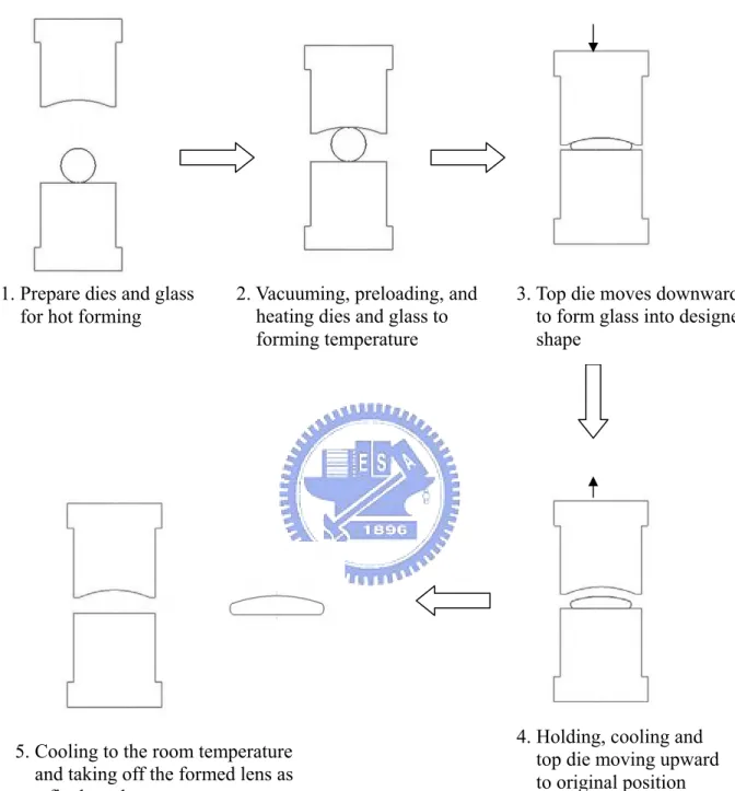
(14) merits of glass molding, like easiness for mass production, cost reduction of labor and time, and simplified steps of process. In general, glass lens molding includes two kinds of methods, which are open-die molding and closed-die molding. The main purpose of closed-die molding is to eliminate the barreling appearance. But the hot forming parameters used in closed-die lens molding process are more complicated and should be well-designed. That is to say, there are several different and complex steps required in forming and cooling stages to control the lens internal stress which may influence the lens geometry and the refractive index of glass material. In this thesis, open-die glass lens molding is chosen in the fabrication process. Fabrication process of glass lens molding can be generalized to three stages (Figure 1.1): (1) Heating: After the dies and glass preform were put into the hot forming working machine, both the top and bottom dies and the glass preform were then heated to the desired temperature (the forming temperature) which is slightly higher than the transition temperature (Tg) of the used optical glass material. (2) Forming: The top die moved downward with a constant velocity in order to press the glass preform to the designed curvature while the glass material became soft. (3) Cooling: Afterwards, the dies and the glass lens were cooled to a preset temperature (below the Tg) and at the same time the top die was released upwardly to the original position. In the end, the dies as well as the glass lens were cooled to the room temperature and the glass lens became a finished product. 3.

(15) It can be seen from several international publications that feasibility of the glass molding process is beyond all doubt. [1]. 1.3 Literature Review Heckele et al. [1] thought that hot embossing is capable of fabricating the optical microstructure and the products have high precision and high quality. As a result of low material flow rate, hot embossing forming can avoid internal stress which may induce scattering centers unfavorable for optical applications. Finally, hot embossing not only has the potential of increasing production rate but also decreases production costs through the enlargement of the molding surface and automation of the molding process. Shishido et al. [2] researched on the closeness between the glass and the master mold in the softening of the glass and found out that the closeness of fit between the glass and the master mold will vary according to the surface tension of the glass. And it has influence on the precision of the softening process. Huang [3] designed and fabricated mold inserts used in hot embossing forming of spherical optical glass lens. And he discussed the surface roughness of products made by different coating materials on the insert surfaces. Hot embossing forming experiments for spherical lens were conducted using FCD1 as the glass material. According to the results from the experiments, the spherical lens products meet the JIS B 7433 standard on curvature radius and there was no residual stress in the center of the lenses as well. 4.

(16) Yi and Jain [4] performed the experimental and numerical analysis of compression molding for aspherical glass lenses. The glass material used in experiments was BK7 and the simulations were performed using a commercial FEM software DEFORMTM-2D. Rigid-viscoplastic was used in their research to model the glass material. Then, results from the experiments were compared with those from FEM analysis. The results showed that it is possible to use FEM as a tool to analyze the fabrication process.. 1.4 Motivation and Objectives As for optical glass lenses, high accuracy and precision is required for many applications. But during the process of glass lens molding, it is agreed that four factors leading to deviations of the final lens curvature that may effect on the qualities of lens imaging. First of all, during the heating stage, geometrical curvature of the die shape may change due to the variation from room temperature to forming temperature. Secondly, the lens may encounter thermal shrinkage because of the cooling cycle in the process of glass lens molding. The third factor is the residual stress inside the formed lens that may cause the deviations of the final lens product. The forth factor is the characteristic of structural relaxation that is related to the viscoelastic nature of glass material. In short, these problems need to be overcome to ensure the quality of final lens products. As a result, the first objective in this thesis is to determine the feasibility of applying finite element analysis to the performance of predicting lens molding process and to outline other issues occurred that 5.

(17) may be helpful in better modeling design in the future. The second objective is to construct a die shape optimization system in order to compensate the geometrical deviations to the original designed curvature for the final lens products. In addition, glass lenses with various radiuses and conic parameters were analyzed and compared to establish the tendency of compensations.. 1.5 Research Method At first, according to experimental results done previously by Huang [3] and Wang [5] in our laboratory, the hot forming conditions of the experiments were adopted for simulations in this research. The results show that there are obvious differences between the geometrical shape of the finished lens product and that of the original design. In order to obtain higher precise geometrical curvature of the finished lens product, the optimization will be performed to automatically compensate the final lens products for the inaccuracies. To perform optimization, a linking program must be coded with Fortran compiler in order to make the connection between the commercial FEA software “MSC. MARC” and the optimization module in IMSL Fortran library. The linking program will read the output file generated from the simulation at first, call the subroutine to do optimization later, and then output the results of the optimization which will be treated as the input file of the finite element analysis. Iterations will continue until convergent solution is obtained.. 6.

(18) 1.6 Thesis Outlines This thesis will be divided into two primary parts. The first part is to perform the finite element analysis to predict the deformed behavior of glass lens at different stages in this molding process. These results can help us to understand more about the lens molding process. The second part is to do die shape optimization in order to get more precision products. Each chapter in this thesis is summarized briefly as follows: Chapter 1 introduces optical lenses and the glass lens molding process, reviews the literature briefly, and describes the motivation, objectives and the research method in this research. Chapter 2 introduces glass material properties because the characteristic nature of glass material is important for the precision of the lens finished products. Chapter 3 constructs the finite element analysis (FEA) module. Thermal-mechanically coupled analysis is selected to model the lens molding process and some results are shown using the commercial FEA software ― MSC. MARC. In the end of Chapter 3, some discussions about the finite element analysis are made. Chapter 4 constructs the integration of the finite element analysis and the optimization so as to do die shape compensation. At the same time, the general compensation method will be introduced shortly. Some optimization results with different aspherical lenses, such as the spherical, parabolic and hyperbolic lenses, will be shown and discussed in the end of the Chapter 4. 7.

(19) Chapter 5 concludes the results of the finite element analysis and the optimization system. Finally, some special and important issue about the glass material model and the die shape compensation are outlined and listed in the future works.. 8.

(20) 1. Prepare dies and glass for hot forming. 2. Vacuuming, preloading, and heating dies and glass to forming temperature. 3. Top die moves downward to form glass into designed shape. 4. Holding, cooling and top die moving upward to original position. 5. Cooling to the room temperature and taking off the formed lens as a final product. Figure 1.1 Open-die molding process of optical glass lens.. 9.

(21) Chapter 2. Optical Glass Material. 2.1 Characteristic of Glasses Most liquids crystallize to solid state when they were cooled to a specified temperature. But there also exists some liquids that do not crystallize but increase their viscosity gradually to become solid eventually. Such kind of materials soften and become liquids while we heat it again, then no constant melting point was observed. Thus, these kind of amorphous condensations are called to be in a “glassy state” and materials with corresponding state are called “glass material”.[6] (Figure 2.1) The glass transition (Tg) is a region of temperature in which molecular rearrangements occur on a scale of minutes or hours, so that the properties of a liquid change which can be easily observed. Below the glass transition temperature, the material is extremely viscous and a solid state exists. Above Tg, the equilibrium state is arrived at easily and the material is in fluid state. Hence, the glass transition is revealed by the change in the temperature dependence of some property of a liquid during cooling. Viscoelasticity is considered an important characteristic of the glass material at the temperature which is higher than its Tg. How to model the viscoelasticity precisely in material property using finite element analysis is really a challenge for engineers.. 2.2 Classifications of Optical Glasses There are more than three hundred types of optical glasses in 10.

(22) worldwide markets. Two different classifications are generally used to distinguish one optical glass from another. One classification is to differentiate chemical composition of the optical glass and the other classification is based on the difference of refractive index and Abbe Number of the optical glass. Accordingly, “Crown glass” and “Flint glass” are two primary types of optical glasses in accordance with the values of the refractive index and Abbe number. The composition of Crown glass includes “BaO”, which has a lower refractive index (nd <1.6) and higher Abbe number(νd >50). The chemical composition of “Flint glass” is primarily “PbO”. The refractive index and Abbe number of Flint glass are respectively higher (nd >1.6) and lower (νd <50) relative to Crown glass. The glass material used in this research is S-FPL52, which is produced from Ohara Corporation (Figure 2.2). Ohara has divided their glasses into several groups [7]. It can be seen from nd–νd diagram that S-FPL52 is a sort of Crown glass.. 2.3 Material Properties of Optical Glasses 2.3.1 Optical Properties As far as optical lens is concerned, optical property is the most important property that may affect the performances of optical lens products. Optical properties are described roughly as follows: (1) Refraction: Light rays are bent when they cross the boundary separating 11.

(23) optical medium a from medium b. Absolute index of refraction by definition can be written as [8] n=. c v. (2.1). , where c stands for the velocity of light in vacuum and v is the velocity in optical media. Relative index of refraction is another kind of expression more commonly used in engineering, which can be expressed as nrelative =. n glass nair. (2.2). , where nglass represent the refractive index of glass while nair is the refractive index of air. (2) Dispersion: The refractive indices nd and ne in the following two formulas are determined by refractive indices for d-line (587.56 nm) and e-line (546.07 nm). The lines of spectrum listed in Table 2.1 are commonly used to test the refractive indices. Taking dispersion into account, it is Abbe number that is generally used to express how much dispersion it is. Consequently, Abbe numbers are determined from the following νd and νe formulas, calculated normally to the second decimal place.. 12.

(24) vd = ve =. nd − 1 n F − nc. (2.3). ne − 1 n F ' − nc '. (2.4). (3) Transimittance: Some optical glasses show remarkable absorption of light near the ultraviolet spectral range. For certain glasses with high refractive index, absorption extends to the visible range. This not only depends on the chemical composition, but also on unavoidable impurities. Some glass materials with few absorption of light are called transparent. Transimittance refers to the level of the absorption of light.. 2.3.2 Mechanical Properties (1) Modulus of Elasticity: Young’s modulus, modulus of rigidity, and Poisson’s ratio of glass materials are determined by measuring the velocities of the longitudinal and transverse elastic waves at room temperature in a well-annealed glass rod. Young’s modulus (E), Modulus of rigidity (G), and Poisson’s ratio (σ) are commonly calculated using the following equations.. 13.

(25) G = ν t2 ρ. Modulus of rigidity. E=. Young ' s Modulus. Bulk Modulus Poisson′s ratio. (2.5). 9 KG 3K + G. 4 2 K = ν1 ⋅ ρ − G 3. σ=. E −1 2G. (2.6) (2.7) (2.8). ,where v1 and vt are velocity of longitudinal and transverse waves, and ρ refers to density. (2) Knoop Hardness (Hk) The indentation hardness of optical glass is determined with the aid of a micro hardness tester. One face of the glass specimen with the necessary thickness is polished. The diamond indentor is formed rhombic to test the hardness using an increased force on the surface of the glass specimen in order to make the permanent deformation occurred. Then, the Knoop hardness can be computed with the following equation: Hk = 1.451. Knoop hardness. F l2. (2.9). , where F and l denote load and length of longer diagonal line (mm) respectively. (3) Viscosity Glasses go through three viscosity ranges between the melting temperature and room temperature (Figure 2.1): the melting range, 14.

(26) the supercooled melt range, and the solidification range. The unit of viscosity is dPa·s or poise in common use. The viscosity of glass constantly increases during the cooling of the melt (about 100~104 dPa·s). A transition from liquid to plastic state can be observed between 104 and 1013 dPa·s. The so-called softening point identifies the plastic range in which glass parts rapidly deform under their own weight. This is the temperature at which glass exhibits a viscosity of 107.6 dPa·s. The glass structure can be described as solidified or frozen above 1013 dPa·s. This value is very important in the annealing of glasses. Another possibility for identifying the transformation range is by evaluating the rate change of relative linear thermal expansion.. 2.3.3 Thermal Properties Thermal properties are essential to processing optical glass for annealing, heat treatment and coating. They include the strain point, annealing point, softening point, transformation point, yield point and thermal conductivity. The transformation region is the temperature range in which glasses gradually transform from their solid state into a “plastic” state. This region of transformation is defined as the transformation temperature (Tg). Viscosity coefficient at this temperature is approximately 1013 dPa·s. Thermal conductivity means the rate of heat transfer inside the material and thermal expansion is the degree of expansion and shrinkage while the external temperature varies. 15.

(27) 2.3.4 Other Properties Chemical property of the optical glass material is another important property in industrial use. Generally speaking, chemical property of the optical glass material involve in the resistance against the moisture moisture, abrasion and acid. When the optical glass material is put into the environment with lots of humidity or chemicals, what will happen is associated with the chemical composition of the glass. In practical use, it is most desirable to manufacture bubble-free optical glasses, but the existence of bubbles to some extent is inevitable. Bubbles in optical glasses vary in size and number from one glass to another due to different compositions and production methods. Compare to a bubble with a given dimension, a larger quantity of bubbles of smaller dimensions is allowable.. 16.

(28) Table 2.1 Wavelengths and sources of some prominent Fraunhofer lines.[8]. Color. Spectral line Wavelength (nm) Element. Infrared. t. 1013.98. Hg. Red helium. r. 706.52. He. Red hydrogen. C. 656.27. H. Red hydrogen. C'. 643.85. Cd. Yellow sodium. D. 589.3. Na. Yellow helium. d. 587.56. He. Green mercury. e. 546.07. Hg. Blue hydrogen. F. 486.13. H. Blue hydrogen. F'. 479.99. Cd. Blue mercury. g. 435.83. Hg. Dark blue. G'. 434.05. H. Violet mercury. h. 404.66. Hg. Ultraviolet. i. 365.0. Hg. 17.

(29) Figure 2.1 Specific volume variation with temperature. 18.

(30) Figure 2.2 nd–νd diagram of optical glasses for glass mold optics [7]. 19.

(31) Chapter 3 Finite Element Analysis 3.1 Introduction of FEA Finite element analysis (FEA) is a kind of numerical analysis methods used to predict the deformation behavior, model the process of fabrication, represent performance of materials, and display stress distribution or velocity field. For a given boundary value problem, finite element analysis utilizes numerical techniques to obtain approximate solution associated with the specified physical system. It is helpful for engineers to use finite element analysis because it can reduce costs and can shorten time of development. Procedure of finite element analysis can be generally divided into preprocessing, analysis and postprocessing. In preprocessing, the engineers plot the geometrical model, define the material property used, select the mesh condition and give the boundary conditions. Additionally, the engineer needs to set up the analytical parameters, such as time step, in simulation controls. As the settings in preprocessing are completed, the input file for analysis will be generated and subsequently submitted to the analysis solver. After the completion of analysis, the engineer can obtain some information about stress distribution, variation of displacement, velocity field, temperature field and so on in the postprocessing stage.. 3.2 FEA Software The FEA software used to model the lens molding process in this thesis is MSC. MARC. MARC is a commercial FEA code for general 20.

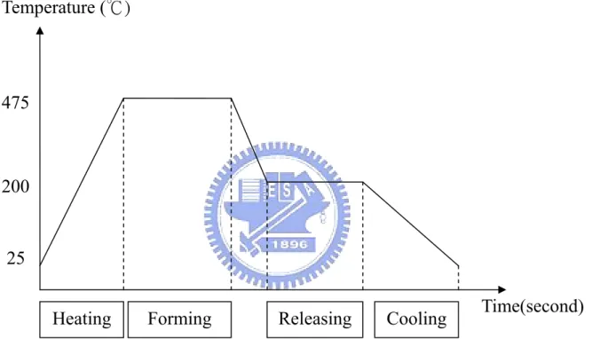
(32) purpose. There are two choices in using MARC as an analyzer. The user can select Mentat as preprocessing and postprocessing. In addition, MSC. AFEA module is another popular choice. In this module, MSC. Patran is taken as preprocessing and postprocessing. Among these two, Mentat provides more detailed choices in analytical settings or simulation controls for users to set up much precisely and is therefore chosen in this research. The solver, MARC, is capable of solving nonlinear deformation behavior taking the viscosity into consideration. Additionally, the capability of determining material parameters from experimental data by curve fitting is also very helpful for engineers to model complex materials, like polymers or glass. The build-in automatic remeshing (rezoning) function can increase the efficiency for solving problems concerning heavy mesh distortion which may lead to premature termination of analysis. [9]. 3.3 Process of Glass Lens Molding The glass lens molding process in the previous experimental works can be simplified into three stages: In the heating stage, the dies and the glass preform are heated to the temperature about 475℃, which is 30℃ higher than the transition temperature of glass “S-FPL52” (445℃). In forming stage, while the dies and the glass are hold at the constant temperature 475℃, the top die move downward with a constant velocity of 0.0483 mm/s. Then, in the final cooling stage, both the dies and the glass are cooled to around 200℃, the top die moves back to its original 21.

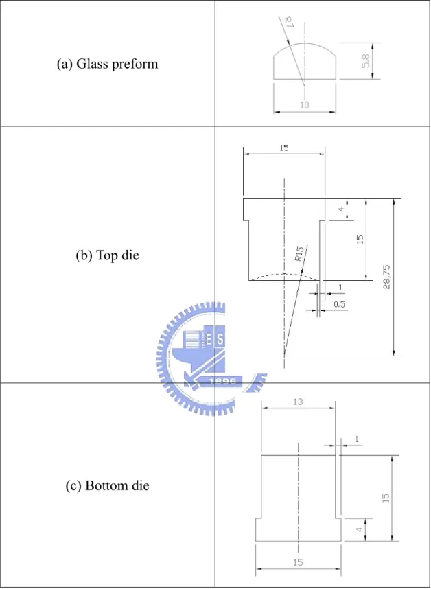
(33) position and eventually they are cooled together to room temperature. (Figure 3.1) All three stages will be considered in the following finite element analysis.. 3.4 Finite Element Analysis Since the process of glass lens molding involves heating and cooling, the analysis type should take the heat transfer effect into account and should be treated as a thermo-mechanical coupled analysis. This section will introduce the geometrical model, material property, and other analytical settings for the coupled analysis using commercial FEA software MSC.MARC.. 3.4.1 Geometrical Model Simplified geometry is helpful for numerical calculation for finite element analysis. Plano-convex lens geometry is selected for this lens molding fabrication process. Because the external appearances of dies and glass preform are symmetric with the central axis, the fabrication processes are therefore treated as an axisymmetric problem. The symmetric axis in MARC by default setting is x axis. A spherical lens whose radius is 15 mm is formed in this lens molding fabrication. The geometric curvature of top die is therefore designed with radius in 15 mm and a glass preform with radius in 7 mm is adopted in this simulation. The detailed sizes of top die, bottom die and glass preform are shown in Figure 3.2.. 22.

(34) 3.4.2 Material Properties Because the flow stress of the glass material varies with strain rate during the forming stages at high temperature. Material properties modeling of glasses are typically regarded as viscoplastic by many researches [4]. Considering the requirement of the geometrical accuracy of the optical lens products, the elastic deformation behavior of the glass lens during the cooling cycle should be taken into account. Therefore, elasto-viscoplastic is used to model the glass material in this thesis. The description of the used nonlinear elasto-viscoplastic material model with formulation is shown below:. ⎧ ⎨ ⎩. σ = E (T )ε , if σ < σ Y σ = 3η (T )ε& , if σ ≥ σ Y. (3.1). ,where E is the temperature-dependent Young’s modulus, T is the specified temperature and σ Y. is the flow stress. η (T ) and ε&. represent the viscosity and strain rate respectively. With respect to the elsto-viscoplatic material model, the glass material behaves itself in linear elasticity while the stress of the glass is smaller than the flow stress. Above the flow stress, the deformation behavior of the glass material depends on the strain rate and viscosity. Moreover, the viscosity changes with the variation of temperature. During the forming stage, temperature of the environment and the glass material is constant and the viscosity accordingly is served as a constant. Flow stress ( σ Y ) had been calculated through the parametric material model in accordance with the 23.

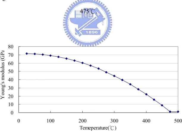
(35) compression experiments conducted in our laboratory (shown in Figure 3.3). In this thesis, the material model is assumed to be the elasto-perfectly plastic since the experimental results agree well with the analytical results. While the forming temperature is set to 475℃ and the specified strain rate is 0.0083 (1/s), the viscosity and the flow stress of the glass material used are 1000 MPa·s and 24.9 MPa respectively. Additionally, Young’s modulus is directly related to the elastic deformation behavior of the material. And for glasses, the Young’s modulus is not constant but is temperature-dependent during the heating and cooling stages [10,11]. The relationships of temperature and Young’s modulus of glass materials can be formulated and expressed by the following equation [10],. Et = E0 − At − Bt 2. (3.2). where Et is the Young’s modulus at temperature t and E0 is the Young’s modulus at room temperature. A and B are the constants depending on the particular glass. Based on the experiments done in our laboratory, Young’s modulus of the glass material S-FPL52 used in this simulation had been measured, which is 1300 MPa at forming temperature 475℃. And the Young’s modulus of the glass material at room temperature is 71700 MPa, provided by Ohara Corporation [7]. With equation (3.2) the constant coefficients A and B are found to be -8.234 and 0.3294 respectively. The relating relationship of the S-FPL52 glass material between the Young’s modulus and temperature can be plotted in Figure 3.4. 24.

(36) In addition, preliminary verifications of the material modeling had been conducted by Tsai in our laboratory to ensure the validities of the material model (refer to Appendix A). Other detailed mechanical and thermal material properties of the dies and glass used in this analysis are listed in Table 3.1.. 3.4.3 Boundary Conditions Figure 3.5 shows the two-dimensional axisymmetric model of lens molding process with the displacement and thermal boundary condition applied to it. The lowest part of the bottom die is fixed in axial direction and the movement of top die as in the actual experiment is given a displacement boundary condition of 2.5mm downwardly. For this simulation, it is assumed that conduction and convection are the primary modes of heat transfer mechanism in thermal-mechanical coupled analysis. A convective heat transfer coefficient of 200 W·(m·℃)-1 and a constant value of the interface heat transfer coefficient of 2800 W·(m·℃)-1 are used to simulate the heat exchange at the contact surfaces between the glass and dies. Many investigators have treated the heat transfer in glass at higher temperatures by a term called effective or apparent thermal conductivity [4], which is a characteristic of the given experimental condition, and hence varies with each setup. A constant value of thermal conductivity is used in this thesis because of the unavailability of thermal data.. 25.

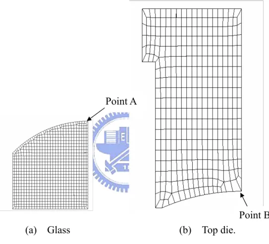
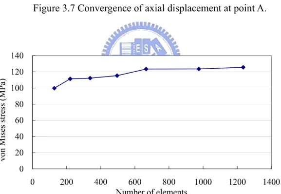
(37) 3.4.4 Contact Surfaces A simplified shear friction model represented by equation (3.3) was used to model the friction effect at the glass-die interface: τ = m ⋅ km. (3.3). , where τ is the shear strength of the interface specified in MPa, m is the shear friction factor (0≤ m ≤1), and km is is the shear yield stress of the softer material specified in MPa. A shear friction coefficient of 1.0 was used to assume that complete sticking taking place between the glass and the dies.. 3.4.5 Mesh Density Tests Four-node axisymmetric, thermo-mechanical coupled, quadrilateral elements (element type number 11 in MARC) were used to model the objects. To do the convergence tests of mesh density, the first thing is to determine the objectives of the convergence tests. In this simulation, variation of the displacement and the distribution of the stress and strain field in the formed lens are important for us. So, the axial displacement at Point A (Figure 3.6) is chosen as the objective of the mesh convergence test of the glass lens. The maximum von Mises stress of top die at point B (Figure 3.6) occurs in the beginning of the cooling cycle and therefore it is selected as the objective of the mesh convergence test of top die. According to the convergence test of mesh condition (Figure 3.7 and Figure 3.8), 800 elements are used to mesh the glass material, which is reasonable to simulate the glass lens. Although more elements can 26.

(38) increase the accuracy of the simulation results, considering the complication in thermo-coupled analysis and the geometric proportion of glass lens to dies, 400 elements are used to mesh the top and bottom die respectively. Additionally, in the next chapter, die shape optimization will be performed to compensate for the form error of the lens. Too many elements of the top die may increase the design variables in the optimization procedure and reduce the efficiency of the convergence of the calculation.. 3.5 Results and Discussions Figure 3.9 shows the configurations of glass and dies corresponding to the heating, forming and cooling stages. Figure 3.10 and Figure 3.11 shows the displacement field of the formed lens. Figure 3.10 displays the axial displacement distribution in the beginning of the cooling cycle with the temperature variation from 480℃ to 300℃. Around 400℃ and above, the axial displacement of the formed glass lens looks like being influenced with the shrinkage of the top die. It is expected that the Young’s modulus of the glass material at high temperature is much smaller than that of the top die. But at around 300℃, there exists an obvious difference seen at between the top die and the glass lens. On the other hand, the displacement variations in radial direction almost vanished at the contact interfaces between the both dies and the glass as a result of the complete sticking friction setting (Figure 3.11). This also causes the barreled appearance. 27.

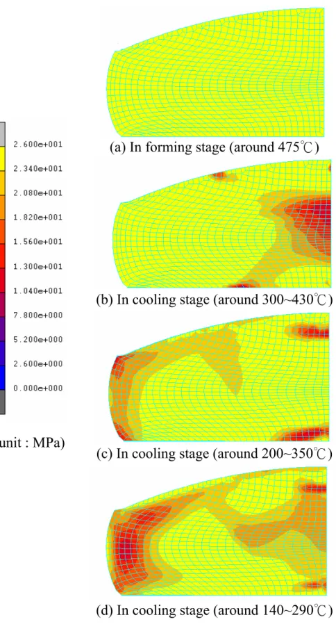
(39) It can be seen obviously from Figure 3.12 and Figure 3.13 that the maximum von Mises stress is around 25 MPa, which is the flow stress given in glass material at 475℃. That means the deformation of glass lens behaved itself in plasticity and could not recovered the appearance to the original one. Figure 3.12 and Figure 3.13 also shows the variation of the von Mises stress distribution inside the formed lens, which decreases with reduction of the temperature. This is the so-called residual stress which can influence the index of the homogeneous refractive of the lens. In practice, the residual stress should be eliminated completely and the procedure to eliminate the residual stress needs to be well-designed in the forming and annealing (cooling) stages. Figure 3.14 shows that the geometrical curve of top die at the end of heating stage differs from the initial designed one. And the displacement in the surface of the top die is not uniform. The results reveal thermal expansion of the top die during the heating stage had resulted in deviations of 0.03096 mm in the center. On the other hand, Figure 3.15 illustrates that there exists an apparent difference in geometry of the formed lens after the cooling stage and before the die releasing, that is 0.0524 mm at the center. Figure 3.16 plots the formed and designed lens curves. Uneven errors are found and plotted in Figure 3.17. The error increases slightly with the distance from the center axis. As a result, regardless of the reasons leading to lens deviations, the following step is to construct a die shape optimization in order to automatically compensate for these deviations in the finished lens products. 28.

(40) Table 3.1 Material properties of dies and glass. Dies Material type. Glass. Elastic Elasto-viscoplastic. Young modulus (GPa). 610. See Figure 3.4. Poison ratio. 0.299. 0.21. Density (kg/m3). 14900. 3550. Thermal conductivity (W·(m·℃)-1). 82. 0.849. Coefficient of thermal expansion (×10-6/℃). 5. Specific heat (J·(kg·℃)-1). 300. Transition temperature. 18 ( ≤ 445℃) 100.4 ( > 445℃) 800 445℃. 29.

(41) Temperature (℃). 475. 200. 25 Heating. Forming. Releasing. Cooling. Figure 3.1 Temperature history diagram. 30. Time(second).

(42) (a) Glass preform. (b) Top die. (c) Bottom die. Figure 3.2 Geometrical model in detailed size of both dies and glass. (Unit : mm). 31.

(43) σ (MPa). ε& = 0.011 (1 / s). σY = 30.0. ε& = 0.0083 (1 / s). σY = 24.9. ε& = 0.0067 (1 / s ). σY = 20.1. ε. Figure 3.3 Relations between stress and strain with different strain rate at 475℃.. Young's modulus (GPa. 80 70 60 50 40 30 20 10 0 0. 100. 200 300 Temeperature(℃). 400. Figure 3.4 Young’s modulus as a function of the temperature.. 32. 500.

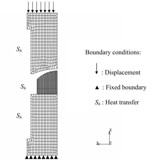
(44) Sh. Boundary conditions: : Displacement. Sh. : Fixed boundary Sh : Heat transfer. Sh. Figure 3.5 Boundary conditions in axisymmetric analysis model. 33.

(45) Point A. Point B (a). Glass. (b). Top die.. Figure 3.6 Points for conducting the mesh density tests.. 34.

(46) Displacement (mm). -2.00 -2.02 -2.04 -2.06 -2.08 -2.10 0. 500. 1000 Number of elements. 1500. 2000. Figure 3.7 Convergence of axial displacement at point A.. 140 von Mises stress (MPa). 120 100 80 60 40 20 0 0. 200. 400. 600 800 1000 Number of elements. 1200. Figure 3.8 Convergence of von Mises stress at point B.. 35. 1400.

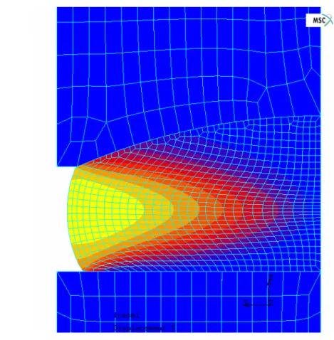
(47) (a) Heating. (b) Forming. (c) Releasing and cooling. Figure 3.9 Simulated process of lens molding.. 36.

(48) (a) T=475℃. (b) T=450℃. (c) T=400℃. (d) T=300℃. (Unit: mm). Figure 3.10 Axial displacement of glass formed lens.. 37.

(49) (unit : mm). Figure 3.11 Radial displacement of glass formed lens(at 475℃).. 38.

(50) (a) In forming stage (around 475℃). (b) In cooling stage (around 300~430℃). (unit : MPa). (c) In cooling stage (around 200~350℃). (d) In cooling stage (around 140~290℃) Figure 3.12 von Mises Stress distribution of formed lens during cooling cycle.. 39.

(51) (e) In cooling stage (around 100~200℃). (f) In cooling stage (around 50~120℃). (unit : MPa). (g) In cooling stage (around 30~60℃). (h) In cooling stage (around 25℃) Figure 3.13 (continued) von Mises Stress distribution of formed lens during cooling cycle.. 40.

(52) Original designed geometry of top die. 0.03096 mm. Die shape expansion after heating stage. (unit:mm) Figure 3.14 Die shape deviation due to thermal expansion. 41.

(53) Central difference = 0.0524 mm. Figure 3.15 Geometrical err of lens curve after cooling stage. 42.

(54) -1.8. y coordinates(mm). -2.0 -2.2 -2.4 -2.6 -2.8. Formed lens curve Designed lens curve. -3.0 -3.2 -3.4 0. 1. 2. 3 4 x coordinates(mm). 5. 6. error (mm). Figure 3.16 Comparison between the designed and formed lens curve.. 0.10 0.09 0.08 0.07 0.06 0.05 0.04 0.03 0.02 0.01 0.00 0. 1. 2. 3 4 x coordinates(mm). 5. Figure 3.17 Error between the designed and formed lens.. 43. 6.

(55) Chapter 4. Die Shape Optimization. 4.1 Introduction In glass lens molding process, there exist several factors which causes the geometrical errors of the final products, for instance, the die expansion during the heating stage and the lens shrinkage in the cooling stage. In order to overcome such problems, a die shape optimization process will be conducted to simulate the process and compensate for deviations automatically. Generally, in industrial practice, engineers consider the deviations of the final products and hence will make an estimation previously in the die and mold shape curve in design. The primary consideration is the shrinkage ratio of the final products to the original design. The shrinkage ratio can be calculated from equation (4.1), where α refer to the shrinkage ratio regarding the forming process. Generally, α is 0.005~0.007. D and M represent the size of the original design and the final products at room temperature.. α=. D−M M. (4.1). Nevertheless, this kind of estimation still can not eliminate the error of the final products entirely because the error occurrence not only depend on the thermal expansion of the workpiece but also concern the complicated mechanism in the manufacturing process. The following steps are to compensate the die and mold shape from the measurements of the errors. The action of compensation usually is not for just one time but 44.

(56) repeated until the goal of error reduction is reached. Therefore, in order to get high precision products, a lot of time and cost are needed. For that reason, so as to increase efficiency of the development, there will be a die compensation procedure constructed in this chapter. This die shape optimization incorporates the finite element analysis into the optimization method. More detailed description of integration procedure will be introduced in section 4.3. First of all, general optimization concept will be introduced in the following section.. 4.2 Fundamental Theory of Optimization In an engineering problem concerning a physical system, there always exist lots of difficulties needed to be overcome and design optimization is a kind of method commonly used to solve such problems. Design optimization refers to the process of finding out some given design variables, which, when used within the model, satisfy prescribed conditions or feasible region regarding the performance of the design and at the same time minimize or maximize an objective function or cost function of the design. Design variables are the variables that can be changed as to the whole design but there always exists lower or upper limit needed to be satisfied. Design variables can be continuous or discontinuous. Objective functions or cost functions refer to the desirable condition that the engineers want to reach. And the feasible region stands for the constraints of the prescribed design. In many engineering applications for process of product design, conflicting objectives or discontinuous design variables, such as cost, weight, deflection, reliability 45.

(57) and so on, should be considered by the designer on purpose of conforming with the reality. A general mathematical model for optimization problem with objectives and constraints is defined as follows: Find a n-vector x = (x1, x2, …, xn) of design variables to minimize an objective function: F(x) = ( x1, x2, ..., xn ). (4.2). subject to the equality constraints hj(x) = ( x1, x2, ..., xn ) = 0, j =1, 2, ..., p. (4.3). and the inequality constraints gi(x) = ( x1, x2, ..., xn ) ≤ 0, i = 1, 2, ..., m. (4.4). and the lower and upper bounds on design variables xkl ≤ xk ≤ xku,. k = 1, 2, ..., n. (4.5). The x1, x2, ..., xn represents a set of design variables used to yield optimal values for the objective functions F(x). The constraints represented by equation (4.3) and equation (4.4) define the feasible design space in connection with the design variable bounds as specified by equation (4.5). The design variable bounds could be incorporated into the formulation as inequality constraints, but their separation in the above formulation will be proved to be the most convenient in the solution procedure developed. The general optimization procedures are shown in 46.

(58) Figure 4.1.. 4.3 The Optimization Algorithm The optimization algorithm adopted in this thesis is the Sequential Quadratic Programming (SQP) method. This method approximates the objective function by a quadratic function. When nonlinear constraints exist, as is the case in most practical design optimization problems, the second order approximation concept is extended to the Lagrangian which is a linear combination of the objective function and the constraint functions. SQP method is often selected as a single objective optimizer with continuous variables for accuracy, reliability and efficiency [12].. 4.4 Optimization Implement The implement selected to perform the optimization in this thesis is the optimization module form IMSL Fortran library. The IMSL Fortran Library consists of two separate but coordinated libraries that allow easy user access. These two libraries are mathematical and statistic Fortran libraries. The Fortran 90 language as well as the FORTRAN 77 language are the standard that can be consulted in this IMSL module. According to the description of optimization algorithm above, “NNLPF” subroutine is used to perform the optimization. This subroutine is coded on the basis of the SQP method discussed above. The users are required to define the design variables, the objective function and the constraints. Instead of giving their gradient functions, the gradient functions of the objective and constraints are calculated automatically by 47.

(59) program during the numerical process.. 4.5 Integration of FEA and Optimization The integration procedure is shown in Figure 4.2 [13]. After the completion of the finite element analysis, its results will be regard as the input file of the optimization and in the meantime the connection program will read the information needed in optimization. Then, the connection program will call “NNLPF” subroutine to calculate the value of the given objective function and the constraints. If it converges and satisfy the preset criterion, the program will terminate the computation and output the results. Otherwise, it will modify the nodes of the die geometrical shape in the input file and go through the finite element analysis again.. 4.6 Formulation of Optimization System 4.6.1 Design Variables In order to perform the die shape optimization, the geometrical shape of the die should be therefore treated as the design variables. In finite element analysis, the positions of the die nodes, which might contact the glass, are served as the design variables in the die shape optimization. (Figure 4.3) The coordinates of the designed die nodes can be presented by the following equation.. y=. x2 2. R + R − (1 + k ) x. 2. + A4 x 4 + A6 x 6 + LL. (4.6). Equation (4.6) is the general formulation of the aspherical curve, 48.

(60) where R is the radius of the curve and k is the conic parameter that stands for the variation of the conic section. While k is equal to 0, it is a spherical curve. When k is smaller than 0 but greater than -1, it is an elliptic curve. k = -1 and k < -1 are parabolic and hyperbolic curves respectively (Figure 4.4). A4 and A6 are the modified coefficient of the aspheric curve. As for a local minimum problem, the initial guess of the design variables is important for looking for the optimal solution of the objective function. Therefore, the initial guess of the design variables in this optimization had been regarded as the values considering the shrinkage ratio as described in the beginning of this chapter because the size error of the design with the shrinkage consideration only is less than that without any compensation. Shrinkage consideration means that if we want to get a lens product with radius in 10 mm, the traditional design will set the radius of the dies in 10.050 mm considering the shrinkage ratio 0.005. Hence, the initial guess of the design variables are then calculated through equation (4.7), yinitial =. xinitial 2 2. Rc + Rc − (1 + k ) xinitial. 2. + errorc. (4.7). where xinitial and yinitial are the radial and axial coordinates of the nodes in the die shape curves. Rc stands for the radius considering the shrinkage ratio listed in Table 4.1. errorc is the error between the original design and that with shrinkage consideration only, which is calculated by RMS (root mean square) function, like equation (4.8). 49.

(61) In this optimization system, the method is to modify the specified node coordinates in the input file of the finite element analysis. While the design variables had been changed, the linking program will calculate value of the objective function by calling the analysis solver.. 4.6.2 Objective Function The choice of objective function of the optimization system in this thesis is to minimize the difference between the original die design and the finished shape of the lens. A RMS (root mean square) function is used to define the object function f as in the following equation: n. f =∑. i =1. [. 1 ( X i − xi ) 2 + (Yi − yi ) 2 n. ]. (4.8). In equation (4.8), (Xi, Yi) refer to the node coordinates of the final lens product at the top surface calculated through the finite element analysis and (xi, yi) are the node coordinates of the expectative designed lens curve calculated from equation (4.6). The minimized function f is the target of the optimization.. 4.6.3 Constraints In order to make a successful completion of the optimization system, the element size should be taken into consideration since the element distortion will result in the termination of finite element analysis. If useless outputs are returned to the optimization system, the results of the optimization may be influenced. Therefore, one third of the element size, 0.15, is considered as the boundaries of design variables. 50.

(62) 4.7 Results and Discussions The Optimization system had been constructed and the numbers of design variables are set to sixteen to eighteen depend on the curves of die shapes. There are three kinds of aspherical lenses including spherical, parabolic, and hyperbolic lenses with three different radiuses that had been selected to perform the die shape optimization in order to find out the trend of the movements of the nodes in the die shape curve. The optimization results of the aspherical lenses are compared with the error of the lens products without any compensation and with traditional shrinkage consideration only. Table 4.2 lists the optimization results of aspherical lens with radius of 10 mm. These results show that error reduction of the radius with shrinkage consideration only can reach 75.23%~80.35%. Optimization results of these kinds of lenses can have 94.60%~98.26% error reductions effect. Figure 4.5 to Figure 4.10 show the comparisons with compensation results of the die shape curve and the related glass lens curve. It can be seen obviously that the glass lens curve with shrinkage consideration only are below the expectative designed curve, which means that the shrinkage ratio 0.005 is too much as far as aspheric lenses with this radius are concerned. But at the nodes near the central axis, the formed lens curves with the shrinkage consideration only agree well with the expectative lens curves. Table 4.3 lists the optimization results of aspherical lens with radius of 15 mm. The results show that error reductions of the radius with 51.

(63) shrinkage consideration only are 69.46%~79.59%. The error reduction of spherical lens with the shrinkage consideration only is significantly greater than other two kinds of aspherical lens. Optimization results of these kinds of lenses can reach 94.76%~96.27% error reductions. Figure 4.11 to Figure 4.16 shows comparisons with compensation results of the die shape curve and the related glass lens curve. Compare the lens curves considering shrinkage only with the expectative ones, shrinkage ratio 0.005 is not enough for this kind of radius. But the lens curves considering shrinkage only agree well with the expectative ones at the nodes away from the central axis. Table 4.4 lists the optimization results of aspherical lenses with radius of 20 mm. The results show that error reductions of this radius with shrinkage consideration are only 40.40%~44.98%. The error reductions of optimization results of these lenses are 92.39%~93.40%. Figure 4.17 to Figure 4.22 shows comparisons with compensation results of the die shape curve and the related glass lens curve. With the increase of the conic parameters (k), the differences of the nodes at lens surface between the expectative curves and those with shrinkage compensation only decrease slightly away from the central axis. As a whole, the error reductions of the shrinkage consideration only and optimization increase with smaller radius. The phenomena of unevenness in the difference between the finished products and the expectative curves become more obvious with the increase of the conic parameter (k). For the optimization system, numbers of the design variables play an 52.

(64) important role in getting better results. According to the comparisons with the optimization results of radiuses from ten to twenty millimeters, the smaller radius it has, the more improvement it can be seen. Table 4.5 lists the results of two different numbers of nodes at curvature of the die shape with radius of 20 mm. These results reveal that increasing number of design variables suitably can get higher error reductions. Hence, increasing the number of the nodes in the die shape curvature is needed with the increase of the designed radius if we want to obtain better improvements of results. On the other hand, increasing the number of the nodes may reduce the efficiency of the convergence in the finite element analysis. So, there still exist trade-offs to determine how many design variables there should be. Figure 4.23 to Figure 4.31 show the convergent history of the optimization results. Altogether, optimization system is proved to be useful and efficient in solving the unevenness of error occurrences and better results of error reduction could be obtained.. 53.

(65) Table 4.1 Radiuses considering shrinkage Radius (mm) Original design(R). 10. 15. 20. Shrinkage consideration only (Rc) (α=0.005). 10.050. 15.075. 20.100. Table 4.2 Comparison with optimization results (R=10 mm) Spherical(k=0) error(mm). error reduction(%). 0.06425. 0.00. Shrinkage consideration only 0.01479. 76.98. without compensation. Optimization. 0.00214. 96.67. Parabolic(k=-1) error(mm). error reduction(%). 0.06194. 0.00. Shrinkage consideration only 0.01217. 80.35. without compensation. Optimization. 0.00108. 98.26. Hyperbolic(k=-3) error(mm). error reduction(%). 0.06144. 0.00. Shrinkage consideration only 0.01522. 75.23. without compensation. Optimization. 0.00332. 54. 94.60.

(66) Table 4.3 Comparison with optimization results (R=15 mm). Spherical(k=0) error(mm). error reduction(%). without compensation. 0.06542. 0.00. Shrinkage consideration only. 0.01335. 79.59. Optimization. 0.00343. 94.76. Parabolic(k=-1) error(mm). error reduction(%). without compensation. 0.06461. 0.00. Shrinkage consideration only. 0.01976. 69.46. Optimization. 0.00244. 96.27. Hyperbolic(k=-3) error(mm). error reduction(%). without compensation. 0.04910. 0.00. Shrinkage consideration only. 0.01289. 73.74. Optimization. 0.00185. 96.22. 55.

(67) Table 4.4 Comparison with optimization results (R=20 mm) Spherical(k=0) error(mm) error reduction(%) without compensation. 0.06471. 0.00. Shrinkage consideration only 0.03857. 40.40. Optimization. 0.00427. 93.40. Parabolic(k=-1) error(mm) error reduction(%) without compensation. 0.06476. 0.00. Shrinkage consideration only 0.03563. 44.98. Optimization. 0.00441. 93.19. Hyperbolic(k=-3) error(mm) error reduction(%) without compensation. 0.06331. 0.00. Shrinkage consideration only. 0.0371. 41.40. Optimization. 0.00482. 92.39. Table 4.5 comparison with results of various number of nodes (R=20 mm) error reduction(%) 16 nodes 26 nodes 40.40 41.62. Spherical (k=0). Shrinkage consideration only Optimization. 93.40. 95.39. Parabolic (k=-1). Shrinkage consideration only. 44.98. 44.11. Optimization. 93.19. 93.81. Hyperbolic (k=-3). Shrinkage consideration only. 41.40. 41.44. Optimization. 92.39. 94.68. 56.

(68) Identify: (1) design variables (2) cost function to be minimized or maximized (3) constraints that must be satisfied Collect data to describe the system. Estimate initial design. Analyze the system. Check the constraints. Does the design satisfy converging criteria? No. Change the design using an optimization method. Figure 4.1 Procedure of optimum design [12]. 57. Yes. stop.

(69) Input file for finite element analysis. Modify the nodes of die geometry shape within input file. Thermo-mechanical coupled analysis. Die shape optimization. Satisfy the converging criteria No. compared with the objective function? Yes Complete and output the results. Figure 4.2 Integration procedure of FEA and optimization. 58.

(70) Design variables. Figure 4.3 Design variables in optimization procedure.. 59.

(71) Y Ellipse (-1<k<0) Sphere (k=0) Ellipse (k>0) Parabola (k=-1) Hyperbola (k<-1). Figure 4.4 Conic section curves.. 60.

(72) y coordinate(mm). 5.6 5.4 5.2 5 4.8 4.6 4.4 4.2 4 3.8 3.6 3.4. Initial design (without compensation) Shrikage consideration only Optimization 0. 1. 2. 3 x coordinate(mm). 4. 5. 6. Figure 4.5 Die shape curve with R =10mm (spherical) 3.6 y coordinate(mm). 3.4 3.2 3 2.8. Without compensation Shrikage consideration only Optimization Expectation. 2.6 2.4 2.2 0. 1. 2. 3 x coordinate(mm). 4. 5. Figure 4.6 Glass formed lens curve with R =10mm (spherical). 61. 6.

(73) y coordinate(mm). 5.6 5.4 5.2 5 4.8 4.6 4.4 4.2 4 3.8 3.6 3.4. Initial design (without compensation) Shrikage consideration only Optimization 0. 1. 2. 3 4 x coordinate(mm). 5. 6. Figure 4.7 Die shape curve with R =10mm (parabolic). 3.6. y coordinate(mm). 3.4 3.2 3 2.8 Without compensation Shrikage consideration only Optimization Expectation. 2.6 2.4 2.2 0. 1. 2. 3 x coordinate(mm). 4. 5. Figure 4.8 Glass formed lens curve with R =10mm (parabolic). 62. 6.

(74) y coordinate(mm). 5.6 5.4 5.2 5 4.8 4.6 4.4 4.2 4 3.8 3.6 3.4. Initial design (without compensation) Shrikage consideration only Optimization 0. 1. 2. 3 x coordinate(mm). 4. 5. 6. Figure 4.9 Die shape curve with R =10mm (hyperbolic). 3.6. y coordinate(mm). 3.4 3.2 3 2.8. Initial design Shrikage consideration only Optimization Expectation. 2.6 2.4 2.2 0. 1. 2. 3 x coordinate(mm). 4. 5. Figure 4.10 Glass formed lens curve with R =10mm (hyperbolic). 63. 6.

(75) 0.6 0.4 y coordinate(mm). 0.2 0 -0.2 -0.4 Initial design (without compensation). -0.6. Shrikage consideration only. -0.8. Optimization. -1 0. 1. 2. 3 4 x coordinate(mm). 5. 6. Figure 4.11 Die shape curve with R =15mm (spherical) -1.8. y coordinate(mm). -2 -2.2 -2.4 -2.6. Without compensation Shrikage consideration only Optimization Expectation. -2.8 -3 -3.2 0. 1. 2. 3 4 x coordinate(mm). 5. 6. Figure 4.12 Glass formed lens curve with R =15mm (spherical). 64.

(76) 0.6. y coordinate(mm). 0.4 0.2 0 -0.2 -0.4. Initial design (without compensation) Shrikage consideration only. -0.6. Optimization. -0.8 0. 1. 2. 3 4 x coordinate(mm). 5. 6. Figure 4.13 Die shape curve with R =15mm (parabolic) -1.8. y coordinate(mm). -2 -2.2 -2.4 -2.6. Without compensation Shrikage consideration only Optimization Expectation. -2.8 -3 -3.2 0. 1. 2. 3 4 x coordinate(mm). 5. 6. Figure 4.14 Glass formed lens curve with R =15mm (parabolic). 65.

(77) 0.6. y coordinate(mm). 0.4 0.2 0 -0.2. Initial design (without compensation). -0.4. Shrikage consideration only. -0.6. Optimization. -0.8 0. 1. 2. 3 4 x coordinate(mm). 5. 6. Figure 4.15 Die shape curve with R =15mm (hyperbolic). -1.8. y coordinate(mm). -2 -2.2 -2.4 -2.6 Without compensation Shrikage consideration only Optimization Expectation. -2.8 -3 -3.2 0. 1. 2. 3 4 x coordinate(mm). 5. 6. Figure 4.16 Glass formed lens curve with R =15mm (hyperbolic). 66.

(78) 7.2 7 y coordinate(mm). 6.8 6.6 6.4 6.2. Initial design (without compensation). 6. Shrikage consideration only. 5.8. Optimization. 5.6 0. 1. 2. 3 4 x coordinate(mm). 5. 6. 7. Figure 4.17 Die shape curve with R =20mm (spherical). 4.2. y coordinate(mm). 4 3.8 3.6 3.4 Without compensation Shrikage consideration only Optimization Expectation. 3.2 3 2.8 0. 1. 2. 3 4 x coordinate(mm). 5. 6. Figure 4.18 Glass formed lens curve with R =20mm (spherical). 67. 7.

(79) 7.2. y coordinate(mm). 7 6.8 6.6 6.4 6.2. Initial design (without compensation) Shrikage consideration only. 6 5.8. Optimization. 5.6 0. 1. 2. 3 4 x coordinate(mm). 5. 6. 7. Figure 4.19 Die shape curve with R =20mm (parabolic). 4.2. y coordinate(mm). 4 3.8 3.6 3.4 Without compensation Shrikage consideration only Optimization Expectation. 3.2 3 2.8 0. 1. 2. 3 4 x coordinate(mm). 5. 6. Figure 4.20 Glass formed lens curve with R =20mm (parabolic). 68. 7.

(80) 7.2. y coordinate(mm). 7 6.8 6.6 6.4 6.2. Initial design (without compensation) Shrikage consideration only Optimization. 6 5.8 5.6 0. 1. 2. 3 4 x coordinate(mm). 5. 6. 7. Figure 4.21 Die shape curve with R =20mm (hyperbolic). 4.2. y coordinate(mm). 4 3.8 3.6 3.4. Without compensation Shrikage consideration only Optimization Expectation. 3.2 3 2.8 0. 1. 2. 3 4 x coordinate(mm). 5. 6. Figure 4.22 Glass formed lens curve with R =20mm (hyperbolic). 69. 7.

(81) value of object function. 0.006 0.005 0.004 0.003 0.002 0.001 0 1. 2. 3. 4. Number of iterations in optimization. Figure 4.23 Convergence of optimization with R =10mm (spherical). Value of object function. 0.0035 0.003 0.0025 0.002 0.0015 0.001 0.0005 0 1. 2. 3. 4. 5. 6. Number of iterations in optimization. Figure 4.24 Convergence of optimization with R =10mm (parabolic). 70.

(82) Value of object function. 0.007 0.006 0.005 0.004 0.003 0.002 0.001 0 1. 2. 3. 4. 5. 6. 7. Number of iterations in optimization. Figure 4.25 Convergence of optimization with R =10mm (hyperbolic). Value of object function. 0.006 0.005 0.004 0.003 0.002 0.001 0 1. 2. 3. 4. Number of iterations in optimization. Figure 4.26 Convergence of optimization with R =15mm (spherical). 71.

(83) value of object function. 0.005 0.0045 0.004 0.0035 0.003 0.0025 0.002 0.0015 0.001 0.0005 0 1. 2. 3. 4. 5. 6. 7. 8. 9. Number of iterations in optimization. Value of object function. Figure 4.27 Convergence of optimization with R =15mm (parabolic). 0.009 0.008 0.007 0.006 0.005 0.004 0.003 0.002 0.001 0 1. 2. 3. 4. 5. Number of iterations in optimization. Figure 4.28 Convergence of optimization with R =15mm (hyperbolic). 72.