A production inventory model which considers the dependence of production rate on demand and inventory level

This article was downloaded by: [National Chiao Tung University 國立交通大學] On: 27 April 2014, At: 23:59

Publisher: Taylor & Francis

Informa Ltd Registered in England and Wales Registered Number: 1072954 Registered office: Mortimer House, 37-41 Mortimer Street, London W1T 3JH, UK

Production Planning & Control: The Management

of Operations

Publication details, including instructions for authors and subscription information:

http://www.tandfonline.com/loi/tppc20

A production inventory model which considers

the dependence of production rate on demand

and inventory level

Chao-Ton Su & Chang-Wang Lin Published online: 15 Nov 2010.

To cite this article: Chao-Ton Su & Chang-Wang Lin (2001) A production inventory model which considers the dependence of production rate on demand and inventory level, Production Planning & Control: The Management of Operations, 12:1, 69-75, DOI: 10.1080/09537280150203997

To link to this article: http://dx.doi.org/10.1080/09537280150203997

PLEASE SCROLL DOWN FOR ARTICLE

Taylor & Francis makes every effort to ensure the accuracy of all the information (the “Content”) contained in the publications on our platform. However, Taylor & Francis, our agents, and our licensors make no representations or warranties whatsoever as to the accuracy, completeness, or suitability for any purpose of the Content. Any opinions and views expressed in this publication are the opinions and views of the authors, and are not the views of or endorsed by Taylor & Francis. The accuracy of the Content should not be relied upon and should be independently verified with primary sources of information. Taylor and Francis shall not be liable for any losses, actions, claims, proceedings, demands, costs, expenses, damages, and other liabilities whatsoever or howsoever caused arising directly or indirectly in connection with, in relation to or arising out of the use of the Content. This article may be used for research, teaching, and private study purposes. Any substantial or systematic reproduction, redistribution, reselling, loan, sub-licensing, systematic supply, or distribution in any form to anyone is expressly forbidden. Terms & Conditions of access and use can be found at http://www.tandfonline.com/page/terms-and-conditions

A production inventory model which considers the

dependence of production rate on demand and

inventory level

CHAO-TON SU and CHANG-WANG LIN

back-log, deteriorating items

Abstract. This study presents a production inventory model

for deteriorating products in which the production rate at any instant depends on the demand and the inventory level. While the demand rate is assumed to decrease exponentially, shortages are allowed and excess demand is backlogged as well. Optimal expressions are obtained for the production scheduling period, maximum inventory level, un® lled order backlog and the total average cost. Some cases of the model are brie¯ y discussed. A numerical example illustrates the practicality of the model. The sensitivity of these solutions to changes in underlying parameter values is also discussed.

1. Introduction

Although many mathematical models have been devel-oped for controlling inventory, a method for formulating

production rate policies for controlling deteriorating items has seldom been mentioned. In practice, demand and inventory level may in¯ uence production. A situation in which the demand decreases (or increases) may cause the manufacturers to decrease (or increase) their production as well. Also, the production rate may either increase or decrease with the inventory level. Thus, the eå ect of inven-tory on production rate warrants further study. In this study, we present a realistic inventory model in which the production rate depends on demand and inventory level, where demand is an exponential decreasing function of time. Such a situation frequently arises in practice. For instance, many items, e.g. electronic components, fashion-able clothes and domestic goods have the rapid sales increase in the beginning; however, they may drastically decline due to either the introduction of new competitive products or changes in consumers’ preferences.

Authors: C.-T. Su and C.-W. Lin, Department of Industrial Engineering and Management,

National Chiao Tung University, Hsinchu, Taiwan, ROC. e-mail: ctsu@cc.nctu.edu.tw

CHAO-TON SU is Professor of the Department of Industrial Engineering and Management,

National Chiao Tung University, Taiwan. He received his PhD from University of Missouri-Columbia, USA. His current research activities include quality engineering, production manage-ment and neural networks in industrial applications. Dr Su has published articles in Computers and

Industrial Engineering, Computers in Industry, International Journal of Industrial Engineering, International Journal of Production Research, International Journal of Production Economics, Production Planning and Control, Integrated Manufacturing Systems, Opsearch, Quality and Reliability Engineering International, International Journal of Quality and Reliability Management, International Journal of Quality Science, International Journal of Systems Science, IEEE Transactions on Components, Packages, and Manufacturing Technology, European Journal of Operational Research, IIE Transactions, Total Quality Management.

CHANG-WANGLINis currently a doctoral candidate in industrial engineering at National Chiao Tung University, Taiwan. His present research interests are in the ® eld of production/inventory control and engineering management, Mr Lin has published articles in Opsearch, Yugoslav Journal of

Operations Research.

Production Planning & Control ISSN 0953± 7287 print/ISSN 1366± 5871 online#2001 Taylor & Francis Ltd http://www.tandf.co.uk/journals

The standard EOQ model assumes a constant and known demand rate over an in® nite planning horizon. Mak (1982) proposed a production lot size inventory model with a uniform demand rate over a ® xed time horizon. However, most items experience a stable demand only during the saturation phase of their life cycle and for ® nite periods of time. Thus, the demand rate varies with time; the EOQ model must obviously be modi® ed. Many studies have extended the EOQ model in order to accommodate time-varying demand patterns. Goswami and Chaudhuri (1991, 1992), Bhunia and Maiti (1997) as well as Bose et al. (1995) assumed a linear trend in demand. Hong et al. (1993) considered an inventory model with time-proportiona l demand, instantaneous replenishment and no shortage. Dave (1989) extended this work by including variable instantaneous demand, discrete opportunities for replenishment and shortages. In addition, Mandal and Phaujdar (1989), and Urban (1992) discussed an inventory level-dependent demand rate. The above investigations did not consider the eå ect of inventory on production rate.

Hollier and Mak (1983) developed inventory replen-ishment policies for deteriorating items with a declining demand. Balkhi and Benkherouf (1996) considered a pro-duction lot size inventory model with arbitrary produc-tion and demand rate which depends on the time function. Goswami and Chaudhuri (1992) developed order-level inventory models for deteriorating items in which the ® nite production rate is proportional to the time-dependent demand rate. Furthermore, Bhunia and Maiti (1997) assumed that the production rate is a vari-able. They also presented inventory models in which the production rate depends on either on-hand inventory or demand. These investigations did not allow for shortages. In this study, we further extend all of the above models to formulate an inventory model for deteriorating items by simultaneously considering the demand rate and the pro-duction rate.

This study attempts to develop a production inventory model by assuming that the deterioration rate is uniform, the ® nite production rate is proportional to both the demand rate and the inventory level, shortages are allowed, and the demand rate decreases exponentially. The total average cost is derived. The optimal expres-sions can be obtained for the production scheduling per-iod, maximum inventory level, un® lled order backlog and total average cost. In addition, some cases are illu-strated by selecting appropriate values for the model’ s various parameters. A numerical example demonstrates the practicality of the model. Finally, sensitivity analysis is performed along with concluding remarks provided as well.

2. Assumptions and notations

The mathematical model of the production inventory problem considered in this paper is developed on the basis of the following assumptions.

(1) A single item is considered over a prescribed period of T units of time, which is subject to a constant deterioration rate.

(2) Demand rate, D…t†, is known and decreases expo-nentially. That is at time t; t ¶ 0, D…t† ˆ Ae¡¶t, A is initial demand rate and ¶ is decreasing rate of the demand, 0 µ ¶ µ 1.

(3) Production rate, P…t†, at any instant depends on both the demand and the inventory level. That is at time t; t ¶ 0, P…t† ˆ a ‡ bD…t† ¡ cI…t†, a > 0, 0 µ b < 1 and 0 µ c < 1,

(4) Deterioration of the units is considered only after they have been received into inventory.

(5) There is no replacement or repair of deteriorated items during a given cycle.

(6) Shortages are allowed and backlogged. The following notations are used:

I…t† inventory level at any time t; t ¶ 0,

³ parameter of the deterioration rate function,

Im maximum inventory level,

Ib un® lled order backlog,

C setup cost for each new cycle,

Cd the cost of a deteriorated item,

Ci inventory carrying cost per unit per month,

Cs shortage cost per unit,

T cycle time,

K the total average cost of system.

3. Mathematical modelling and analysis

Initially the stock is zero. The production inventory level starts at a time t ˆ 0 and reaches Im maximum

level after t1 time units have elapsed. Then the

produc-tion is stopped, the stock level declines continuously and the inventory level becomes zero at time t ˆ t2. Now

shortages start developing and accumulate to the level

Ibat time t ˆ t3. At this instant of time, fresh production

starts to clear the backlog by the time t ˆ t4ˆ T. Our

purpose is to ® nd out the optimal values of t1, t2, t3, t4, Im

and Ib that minimize K over the time horizon [0, T].

The diå erential equations governing the stock status during the period 0 µ t µ T can be written as:

dI…t†

dt ˆ a ‡ …b ¡ 1†A e

¡¶t_{¡ …c ‡ ³†I…t†; 0 µ t µ t} 1; …1†

70 C.-T. Su and C.-W. Lin

dI…t† dt ˆ ¡A e¡¶t¡ ³I…t†; t1µ t µ t2; …2† dI…t† dt ˆ ¡A e ¡¶t_{; t} 2µ t µ t3; …3† and dI…t† dt ˆ a ‡ …b ¡ 1†A e ¡¶t_{¡ cI …t†; t} 3µ t µ t4: …4†

Using the various boundary conditions, i.e.

I…t† ˆ 0 at t ˆ 0; t2 and T; …5†

I…t1† ˆ Imand ¡ I…t3† ˆ Ib; …6†

and after adjusting for the constant of integration, tions (1)± (4) are clearly equivalent to the following equa-tions I…t† ˆ a c ‡ ³‰1 ¡ e ¡…c‡³†t_{Š ‡}A…1 ¡ b† ¶¡ c ¡ ³‰e ¡¶t_{¡ e}¡…c‡³†t_Š; 0 µ t µ t1; …7† I…t† ˆAe ¡¶t ¶¡ ³‰1 ¡ e ¡…¶¡³†…t2¡t†_{Š; t} 1 µ t µ t2; …8† I…t† ˆA ¶ …e ¡¶t_{¡ 1†; t} 2µ t µ t3; …9† and I…t† ˆ ¡a c ‰e c…t4¡t†_{¡ 1Š ¡}A…1 ¡ b† ¶¡ c e ¡¶t_‰e¡…¶¡c†…t4¡t†_{¡ 1Š;} t3µ t µ t4: …10†

From equations (5) and (6), we derive

Imˆ a c ‡ ³‰1 ¡ e ¡…c‡³†t1_{Š ‡}A…1 ¡ b† ¶¡ c ¡ ³‰e ¡¶t1_{¡ e}¡…c‡³†t1_Š ˆ A ¶¡ ³‰1 ¡ e ¡…¶¡³†t2_{Š; …11†} and Ibˆ A ¶ …1 ¡ e ¡¶t3_{† ˆ}a c…e ct4_{¡ 1† ‡}A…1 ¡ b† ¶¡ c ‰e ¡…¶¡c†t4_{¡ 1Š:} …12† Thus, t₁ and t₂ are related by the equation

t2ˆ R…t1† ˆ 1 ³¡ ¶ln 1 ¡ a…¶ ¡ ³† A…c ‡ ³†‰1 ¡ e ¡…c‡³†t1_Š µ ¡…1 ¡ b†…¶ ¡ ³† ¶¡ c ¡ ³ ‰e ¡¶t1_{¡ e}¡…c‡³†t1_Š ¶ : …13†

Again t3 and t4 are related by the equation

t3ˆ R…t4† ˆ ¡ 1 ¶ln 1 ¡ a¶ Ac…e ct4_{¡ 1†} µ ¡…1 ¡ b†¶ ¶¡ c ‰e ¡…¶¡c†t4_{¡ 1Š} ¶ : …14†

The deterioration cost for the period (0; T) is

Cd …t1 0 ³I…t† dt ‡ …t2 t1 ³I…t† dt ³ ´ ˆ Cd …t1 0 a³ c ‡ ³‰1 ¡ e ¡…c‡³†t_Š µ » ‡A³…1 ¡ b† ¶¡ c ¡ ³ ‰e ¡¶t_{¡ e}¡…c‡³†t_Š ¶ dt ‡ …t2 t1 A³ ¶¡ ³‰e ¡¶t_{¡ e}¡…¶¡³†t2_e¡³t_{Š dt} ¼ ; …15† The inventory carrying cost over the period (0; T) is

Ci …t1 0 I…t† dt ‡ …t2 t1 I…t† dt µ ¶ ˆ Ci …t1 0 a c ‡ ³…1 ¡ e ¡…c‡³†t_† µ ‡ A…1 ¡ b† ¶¡ c ¡ ³ …e ¡¶t_{¡ e}¡…c‡³†t_† ¶ dt ‡ Ci …t2 t1 A ¶¡ ³e ¡¶t_{‰1 ¡ e}¡…¶¡³†…t2¡t†_{Š dt; …16†}

and the shortage cost can be written as

Cs ¡ …t3 t2 I…t† dt ¡ …t4 t3 I…t† dt " # ˆ Cs …t3 t2 A ¶…1 ¡ e ¡¶t_{† dt ‡} …t4 t3 µ a c …e c…t4¡t†_{¡ 1†} ( ‡A…1 ¡ b†e ¡¶t ¶¡ c …e ¡…¶¡c†…t4¡t†_{¡ 1†} ¶ dt ¼ : …17†

Hence, the total average cost of the inventory system is

K ˆ setup cost ‡ deterioration cost

‡ inventory carrying cost ‡ shortage cost ˆ C T ‡ …³Cd‡ Ci† T a c ‡ ³ t1‡ 1 c ‡ ³…e ¡…c‡³†t1_{¡ 1†} µ ¶ » ‡A…1 ¡ b† ¶¡ c ¡ ³ µ 1 c ‡ ³…e ¡…c‡³†t1_{¡ 1†}

Production inventory model

¡1 ¶ …e ¡¶t1_{¡ 1†} ¶ ‡ A ¶¡ ³ £ 1 ¶ …1 ¡ e ¡¶t2_{† ‡}1 ³‰e ¡¶t2_{¡ e}¡…¶¡³†t2_Š µ ¶¼ ‡Cs T » At3 ¶ ‡ A ¶2 …e ¡¶t3_{¡ 1† ‡}a c µ 1 c …e ct4_{¡ 1† ¡ t} 4 ¶ ‡A…1 ¡ b† ¶¡ c 1 ¶…e ¡¶t4_{¡ 1† ¡}1 c…e ¡¶t4_{¡ e}¡…¶¡c†t4_† µ ¶¼ : …18†

4. The solution procedure

Diå erentiating the total average cost K given by equa-tion (18) with respect to t1 and t4 and then equating to

zero we ® nd the following two equations. ¡ C T2 ‰1 ‡ R0…t1†Š ‡…³Cd‡ Ci† T » a c ‡ ³…1 ¡ e ¡…c‡³†t1_† ‡ A…1 ¡ b† ¶¡ c ¡ ³‰e ¡¶t1_{¡ e}¡…c‡³†t1_Š ‡AR 0_…t 1† ¶¡ ³ µ e¡¶R…t1†_‡¶¡ ³ ³ e ¡…¶¡³†R…t1†_¡¶ ³ e ¡¶R…t1† ¶¼ ¡…³Cd‡ Ci† T2 » a c ‡ ³ µ t1‡ 1 c ‡ ³…e ¡…c‡³†t1_{¡ 1†} ¶ ‡ A…1 ¡ b† ¶¡ c ¡ ³ µ 1 c ‡ ³…e ¡…c‡³†t1_{¡ 1†} ¡1 ¶…e ¡¶t1_{¡ 1†} ¶ ‡ A ¶¡ ³ µ 1 ¶…1 ¡ e ¡¶t2_† ‡1 ³‰e ¡¶t2_{¡ e}¡…¶¡³†t2_Š ¶¼ ‰1 ‡ R0…t1†Š ¡ Cs 2T2 » At3 ¶ ‡ A ¶2 …e¡¶t3¡ 1† ‡ a c 1 c…e ct4_{¡ 1† ¡ t} 4 µ ¶ ‡A…1 ¡ b† ¶¡ c 1 ¶…e ¡¶t4_{¡ 1† ¡}1 c …e ¡¶t4_{¡ e}¡…¶¡c†t4_† ¶¼ µ £ ‰1 ‡ R0…t1†Š ˆ 0; …19† and ¡ C T2‰1 ‡ R0…t4†Š ¡…³Cd‡ Ci† T2 £ » a c ‡ ³ t1‡ 1 c ‡ ³ …e ¡…c‡³†t1_{¡ 1†} µ ¶ ‡A…1 ¡ b† ¶¡ c ¡ ³ 1 c ‡ ³ …e ¡…c‡³†t1_{¡ 1† ¡}1 ¶ …e ¡¶t1_{¡ 1†} µ ¶ ‡ A ¶¡ ³ µ 1 ¶…1 ¡ e ¡¶t2_† ‡1 ³‰e ¡¶t2_{¡ e}¡…¶¡³†t2 ¶¼ ‰1 ‡ R0…t4†Š ‡Cs T » A ¶ R 0_…t 4†…1 ¡ e¡¶R…t4†† ‡ a c…e ct4_{¡ 1†} ‡ A…1 ¡ b† µ e¡¶t4 c ‡ e ¡…¶¡c†t4 ¶¼ ¡ Cs 2T2 » At3 ¶ ‡ A ¶2…e ¡¶t3_{¡ 1† ‡}a c 1 c …e ct4_{¡ 1† ¡ t} 4 µ ¶ ‡A…1 ¡ b†_¶ ¡ c 1 ¶ …e ¡¶t4_{¡ 1† ¡}1 c …e ¡¶t4_{¡ e}¡…¶¡c†t4_† µ ¶¼ £ ‰1 ‡ R0…t4†Š ˆ 0; …20†

the detail of R…tj† and R0…tj† are given in the Appendix. The pair (t1;t4) will be an optimal solution provided

the following suæ cient conditions are satis® ed @2K @t2 1 > 0; @ 2_K @t2 4 > 0 and @ 2_K @t2 1 £@ 2_K @t2 4 ¡ @ 2_K @t1@t4 ³ ´2 > 0: We obtain two simultaneous non-linear equations in optimal values of t1 and t4 by the Newton-Raphson

(NR) method using a computer. The optimal values of

t2, t3, Im, Iband the minimum total average cost K can be

obtained from equations (11)± (14) and (18), respec-tively.

5. Case illustrations

In this section, we study some important cases that follow from the problem considered in the previous sections.

5.1. Case A. Production rate depends on demand

P…t† ˆ a ‡ bD…t†; …b 6ˆ 0; c ˆ 0†

Arguing as in equation (18) above, the basic conditions for this model becomes

lim c!0 K ˆ C T‡ …³Cd‡ Ci† T » a ³ µ t1‡ 1 ³…e ¡³t1_{¡ 1†} ¶ ‡A…1 ¡ b† ¶¡ ³ µ 1 ³ …e ¡³t1_{¡ 1† ¡}1 ¶…e ¡¶t1_{¡ 1†} ¶ 72 C.-T. Su and C.-W. Lin

‡ A ¶¡ ³ 1 ¶…1 ¡ e ¡¶t2_{† ‡}1 ³‰e ¡¶t2_{¡ e}¡…¶¡³†t2_Š ¶¼ µ ‡CsA ¶T µ t3‡ 1 ¶…e ¡¶t3_{¡ 1†} ¶ ‡aCst 2 4 2T ‡ ACs…1 ¡ b† ¶T 1 ¶ e ¡¶t4_{¡ 1} ¡ ¢ ‡ t4e¡¶t4 µ ¶ : …21†

5.2. Case B. Production rate depends on inventory

P…t† ˆ a ¡ cI …t†; …b ˆ 0; c 6ˆ 0† In this case, equation (18) reduces to

K ˆ C T‡ …³Cd‡ Ci† T » a c ‡ ³ µ t1‡ 1 c ‡ ³…e ¡…c‡³†t1_{¡ 1†} ¶ ‡ A ¶¡ c ¡ ³ µ 1 c ‡ ³…e ¡…c‡³†t1_{¡ 1†} ¡1 ¶…e ¡¶t1_{¡ 1†} ¶ ‡ A ¶¡ ³ µ 1 ¶…1 ¡ e ¡¶t2_† ‡1 ³‰e ¡¶t2_{¡ e}¡…¶¡³†t2_Š ¶¼ ‡Cs T » At3 ¶ ‡ A ¶2…e ¡¶t3_{¡ 1† ‡}a c 1 c…e ct4_{¡ 1† ¡ t} 4 µ ¶ ‡ A ¶¡ c 1 ¶ …e ¡¶t4_{¡ 1† ¡}1 c …e ¡¶t4_{¡ e}¡…¶¡c†t4_† µ ¶¼ :…22†

5.3. Case C. Production rate is uniform

P…t† ˆ a; …b ˆ 0; c ˆ 0†

Substituting the expression of this type of demand into equation (18), we can obtain

lim b;c!0K ˆ C T‡ …³Cd‡ Ci† T » a ³ µ t1‡ 1 ³…e ¡³t1_{¡ 1†} ¶ ‡ A ¶¡ ³ 1 ³…e ¡³t1_{¡ 1†}1 ¶ …e ¡¶t1_{¡ 1†} µ ¶ ‡ A ¶¡ ³ 1 ¶ …1 ¡ e ¡¶t2_{† ‡}1 ³‰e ¡¶t2_{¡ e}¡…¶¡³†t2_Š µ ¶¼ ‡CsA ¶T t3‡ 1 ¶…e ¡¶t3_{¡ 1†} µ ¶ ‡aCst 2 4 2T ‡ ACs ¶T 1 ¶…e ¡¶t4_{¡ 1† ‡ t} 4e¡¶t4 µ ¶ ; …23†

where the decreasing rate of the demand ¶ ! 0 and e³t_{ 1 ‡ ³t ‡ ³}2

t2=2, we then obtain the same model as that given by Mak (1982). Equation (23) for the total average cost of the system is:

K ˆC T‡ …³Cd‡ Ci† T …a ¡ A†t21 2 ‡ At22 2 µ ¶ ‡ACst 2 3 2T ‡ …a ¡ A†Cst24 2T ; …24† where t2ˆ 1 ³ln 1 ‡ ³ ³ a A¡ 1 ´ t1¡ ³t21 2 ³ ´ µ ¶ ; and t3ˆ t4 ³ a A¡ 1 ´ :

Next, if we assume ³ ˆ 0, the model changes to an EOQ model. In this situation, the cost function becomes

K ˆ C T ‡ Ci T …a ¡ A†t21 2 ‡ At22 2 µ ¶ ‡Cs T At23 2 ‡ …a ¡ A†t42 2 µ ¶ ; ˆ C T ‡ CiIm2 2T £ a A…a ¡ A†‡ CsIb2 2T £ a A…a ¡ A†: …25† where t2ˆ a A¡ 1 ± ² t1; and t3ˆ t4 a A¡ 1 ± ² : From equations (11) and (12), we derive

Imˆ …a ¡ A†t1; and Ibˆ …a ¡ A†t4:

6. Numerical example and sensitivity analysis

A numerical example is presented in the following to illustrate the practicality of the proposed model. Assume that an inventory system’ s demand rate decreases nega-tive exponentially in accordance with the equation

D…t† ˆ 200e¡¶t;

and the values of various variables are a ˆ 200 units/ month, Cdˆ 3=unit, b ˆ 0:2, c ˆ 0:2, Cs ˆ 10/unit,

C ˆ 100 for each new cycle, Ciˆ 1/unit/month,

¶ˆ 0:3, ³ ˆ 0:05. The optimum values are calculated for the model and the values are compared using diå er-ent parameters b and c, as shown in table 1. For our model, the optimal production scheduling period is 0.930 month and the total average cost is $123.938, thereby dominating the other three situations.

Now, consider a situation in which only one of the parameter values changes by a ® xed proportion; the other parameters remain unchanged. The following

sen-Production inventory model

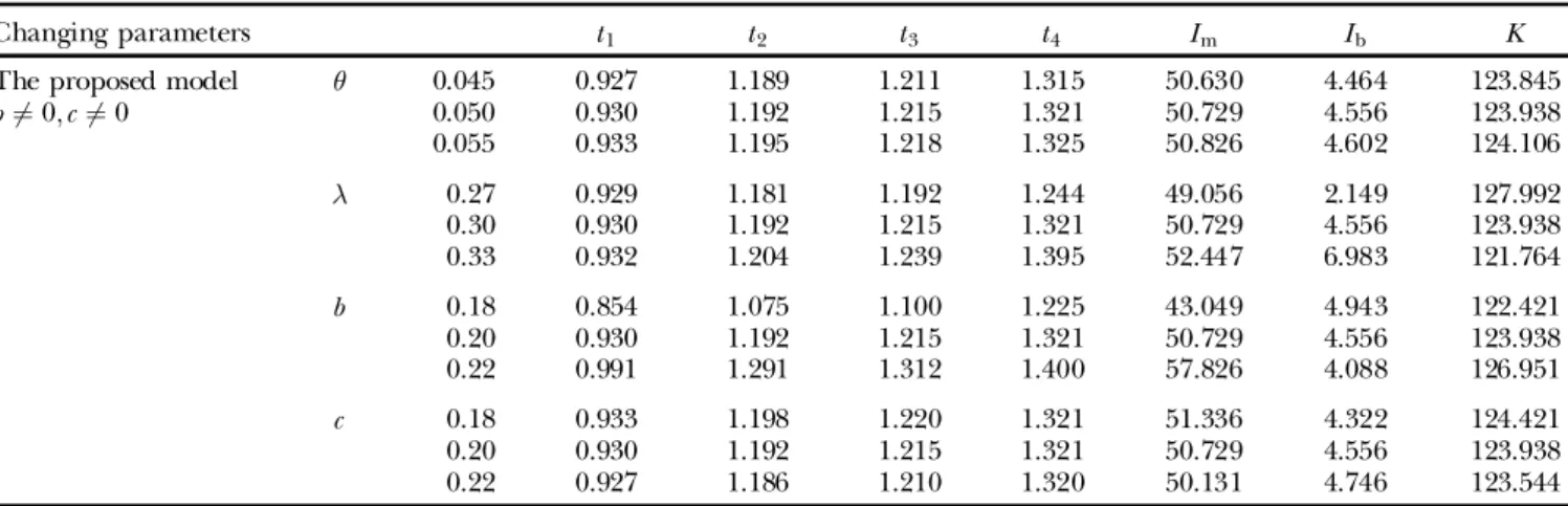
sitivity measures are then calculated for 10% changes in the parameters on either side. Table 2 summarizes these results. Based on the sensitivity analysis, we can infer the following.

(1) An increase in parameters b, ³, ¶ and a decrease in parameter c cause increases in the optimal produc-tion scheduling period t1and the maximum

inven-tory level Im.

(2) An increase in parameters c, ³, ¶ and a decrease in parameter b cause an increase in the un® lled order backlog Ib.

(3) An increase in parameters b, ³ and a decrease in parameters c, ¶ cause an increase in the total aver-age inventory cost K.

(4) The total average inventory cost K increases with an increase in parameters b, ³ and a decrease in parameters c, ¶. Of course, the change in K is small even for a signi® cant change in the value of ¶.

(5) The optimal production scheduling period t1 is

more sensitive to the parameter b than others. It is the intention of this result to provide managers with simple guidelines for determining the production scheduling period. Furthermore, because diå erent par-ameters are involved in this problem, the decision-maker is faced with the diæ cult task of accurately esti-mating these parameters. The above study is robust in

the sense that the decision-maker is provided with a range of parameter values, instead of speci® c ones, for which one mode of production is preferred.

7. Conclusion

Two aspects of deriving inventory models have received increasing interest: the demand rate and the production rate. In this study, we present a production inventory model for deteriorating items by considering that the production rate depends on demand and inven-tory level. The demand rate is assumed to decrease expo-nentially. The developed model is solved by using the Newton± Raphson method. Results presented herein pro-vide a valuable reference for decision-makers in planning production and controlling inventory. A numerical ex-ample demonstrates that applying the proposed model can minimize the total average inventory cost and result in a relatively small production scheduling period. In addition, sensitivity analysis is performed to examine the eå ect of the parameters. According to those results, the proposed model is more sensitive with respect to the parameter b than others. The analysis provided in this study can be very useful for managers in deciding whether they should have a continuous production pol-icy. A future study should incorporate more realistic assumptions into the proposed model, e.g. variable de-terioration rate and stochastic nature of demand. 74 C.-T. Su and C.-W. Lin

Table 1. An illustrative example.

Cases t1 t2 t3 t4 Im Ib K

b 6ˆ 0; c 6ˆ 0 0.930 1.192 1.215 1.321 50.729 4.556 123.938

b 6ˆ 0; c ˆ 0 0.967 1.267 1.278 1.333 57.848 2.272 133.312

b ˆ 0; c 6ˆ 0 3.208 4.198 4.280 5.006 175.430 16.216 164.431

b ˆ 0; c ˆ 0 3.208 4.473 4.574 5.273 216.926 14.724 368.157

Table 2. Eå ects of parameters on the production inventory system.

Changing parameters t1 t2 t3 t4 Im Ib K

The proposed model ³ 0.045 0.927 1.189 1.211 1.315 50.630 4.464 123.845

b 6ˆ 0; c 6ˆ 0 0.050 0.930 1.192 1.215 1.321 50.729 4.556 123.938 0.055 0.933 1.195 1.218 1.325 50.826 4.602 124.106 ¶ 0.27 0.929 1.181 1.192 1.244 49.056 2.149 127.992 0.30 0.930 1.192 1.215 1.321 50.729 4.556 123.938 0.33 0.932 1.204 1.239 1.395 52.447 6.983 121.764 b 0.18 0.854 1.075 1.100 1.225 43.049 4.943 122.421 0.20 0.930 1.192 1.215 1.321 50.729 4.556 123.938 0.22 0.991 1.291 1.312 1.400 57.826 4.088 126.951 c 0.18 0.933 1.198 1.220 1.321 51.336 4.322 124.421 0.20 0.930 1.192 1.215 1.321 50.729 4.556 123.938 0.22 0.927 1.186 1.210 1.320 50.131 4.746 123.544

Acknowledgements

The authors would like to thank the National Science Council of the ROC for ® nancial support of this manu-script under Contract no. NSC-88-2213-E-009-042 .

Appendix

Taking the derivative of equations (13) and (14), we obtain R0…t1† ˆ …­ ¡ ¬†…c ‡ ³†e ¡…c‡³†t1_{‡ ¶­ e}¡¶t1 …³ ¡ ¶†f1 ¡ ¬‰1 ¡ e¡…c‡³†t1_{Š ¡ ­ ‰e}¡¶t1_{¡ e}¡…c‡³†t1_Šg; …A1† where ¬ˆ a…¶ ¡ c† A ‡ c ‡ ³; and ­ ˆ …1 ¡ b†…¶ ¡ ³† ¶¡ c ¡ ³ : and R0…t4† ˆ mce ct4_{¡ n…¶ ¡ c†e}¡…¶¡c†t4

¶f1 ¡ m…ect4_{¡ 1† ¡ n‰e}¡…¶¡c†t4_{¡ 1Šg:} …A2† where m ˆa¶ Ac; and n ˆ …1 ¡ b†¶ ¶¡ c : References

BALKHI, Z. T., and BE NKHEROUF, L., 1996, A production lot

size inventory model for deteriorating items and arbitrary

production and demand rates. European Journal of Operational

Research, 92, 302± 309.

BHINIA, A. K., and MAITI, M., 1997, Deterministic inventory

models for variable production. Journal of the Operational

Research Society, 48, 221± 224.

BOSE, S., GOSW AMI, A., and CHAUDHURI, K. S., 1995, An

EOQ model for deteriorating items with linear time-depen-dent demand rate and shortage under in¯ ation and time discounting. Journal of the Operational Research Society, 46, 771± 782.

DAVE, U., 1989, A deterministic lot-size inventory model with

shortages and a linear trend in demand. Naval Research

Logistics, 36, 507± 514.

GOSW AMI, A., and CHAUDHURI, K. S., 1991, EOQ model for an

inventory with a linear trend in demand and ® nite rate of replenishment considering shortages. International Journal of

Systems Science, 22, 181± 187.

GOSW AMI, A., and CHAUDHURI, K. S., 1992, Variations of

order-level inventory models for deteriorating items.

International Journal of Production Economics, 27, 111± 117.

HOLLIE R, R. H., and MAK, K. L., 1983, Inventory

replenish-ment policies for deteriorating items in a declining market.

International Journal of Production Research, 21, 813± 826.

HONG, J. D., CAVAL IE R, T. M., and HAYY A, J. C., 1993, On the

(t; Sj) policy in an integrated production/inventory model

with time-proportional demand. European Journal of Operational Research, 69, 154± 165.

MAK, K. L., 1982, A production lot size inventory model for

deteriorating items. Computers and Industrial Engineering, 6, 309± 317.

MANDAL, B. N., and PHAUJ DA R, S., 1989, An inventory

model for deteriorating items and stock-dependent con-sumption rate. Journal of the Operational Research Society, 40, 483± 488.

URBAN, T. L., 1992, An inventory model with an

inventory-level-dependent demand rate and relaxed terminal con-ditions. Journal of the Operational Research Society, 43, 721± 724.

Production inventory model