寬頻多入多出直接轉換傳收機之射頻劣化效應估算與補償技術

(1)

國立交通大學

電信工程研究所

博士論文

寬頻多入多出直接轉換傳收機之

射頻劣化效應估算與補償技術

On the Radio Impairment Estimation and

Compensation Techniques for Wideband

MIMO Direct-Conversion Transceivers

研究生：許宸睿

指導教授：沈文和博士

王忠炫博士

(2)

寬頻多入多出直接轉換傳收機之射頻劣化效應

估算與補償技術

On the Radio Impairment Estimation and

Compensation Techniques for Wideband MIMO

Direct-Conversion Transceivers

研究生：許宸睿

Student：Chen-Jui Hsu

指導教授：沈文和博士 Advisor：Dr. Wern-Ho Sheen

王忠炫博士 Dr. Chung-Hsuan Wang

國立交通大學

電信工程研究所

博士論文

A Dissertation

Submitted to Institute of Communication Engineering

College of Electrical and Computer Engineering

National Chiao Tung University

in Partial Fulfillment of the Requirements

for the Degree of Doctor of Philosophy

in

Communication Engineering

Hsinchu, Taiwan

(3)

寬頻多入多出直接轉換傳收機之射頻劣化效應

估算與補償技術

研究生：許宸睿指導教授：沈文和博士

王忠炫博士

國立交通大學

電信工程學系

摘要

在無線通訊傳收機射頻架構設計中，直接轉換架構(direct-conversion radio architecture)是一個具有低成本，低功率消耗和小體積的類比前端設計。然而，此架構卻會產生額外的射頻劣化效應，諸如 I-Q 失衡(I-Q Imbalance)與直流偏移(dc offset)等。這些劣化效應加上所有射頻架構都會產生的頻率偏移(frequency offset)，若無適當的補償，對通訊系統將造成嚴重的效能損失。此篇論文旨在針對多入多出(multiple input, multiple output, MIMO)直接轉換傳收機之射頻劣化效應估算與補償技術做深入研究。基本而言，射頻劣化效應估算與補償技術可分為兩類：第一類為估算補償技術，另一類則是自我校正技術。估算補償技術是在通訊傳輸中，在接收機端去除接收訊號的射頻劣化效應之技術;而自我校正技術則是在通訊傳輸前去除本身射頻劣化效應之技術。此兩類技術皆在本論文中做深入研究；所探討的射頻劣化效應包括了不隨頻率變動的 I-Q 失衡(frequency-independent I-Q imbalance)、隨頻率變動的 I-Q 失衡(frequency-dependent I-Q imbalance)、直流偏移與頻率偏移。

本篇論文在估算補償技術研究方面，探討在多入多出通訊系統下的傳送機與接收機之射頻劣化效應估算與消除方法。首先提出了一個二階段干擾消除架構：在第一階段消除接收端產生之 I-Q 失衡、頻率偏移與直流偏移，而在第二階段消除傳送端產生之 I-Q 失衡。此

(4)

二階段消除架構能適用於各種多入多出之運作模式，包括了空間多工、時空區塊編碼與傳送端波束成形等技術，以及任意的傳送天線數與接收天線數。此外，此架構也概括了各種通訊應用下的消除架構，諸如應用於無線點對點對等(wireless peer-to-peer)通訊、上行鏈路 (uplink)與下行鏈路(downlink)行動通訊。接著我們提出多種參數估算方法，第一種為在最小平方準則下最佳之聯合參數估算方法，分析指出此方法為不偏估計器(unbiased estimator) 以及在有興趣範圍的訊號雜訊比(SNR)下其效能可達到 Cramér-Rao 下限(lower bounds)，但也是最高複雜度的。因此，我們設計其它多種低複雜度估測器，包含了特殊角度旋轉週期訓練設計、直流偏移與頻率偏移簡化估測器與藉由週期訓練協助之低複雜度遞迴估算法。電腦模擬顯示低複雜度設計所造成之效能損失幾乎可被忽略，與現今文獻所提之技術做比較，本論文所提之技術能擁有更低錯誤率以及較短之訓練符元長度需求。在自我校正技術方面，本論文提出一個新的時域方法(time-domain method)，在迴路 (feedback loop)不需要專門額外的類比硬體電路下，能夠同時自我校正傳送機與接收機之射頻劣化效應。此時域方法適用於各類的通訊系統並能同時校正不隨頻率變動與隨頻率變動的 I-Q 失衡和直流偏移。此外，我們亦提出最佳訓練數列化之設計方法，並由分析與模擬驗證了此方法之正確性與有效性。

(5)

On the Radio Impairment Estimation and

Compensation Techniques for Wideband MIMO

Direct-Conversion Transceivers

Student: Chen-Jui Hsu Advisor: Dr. Wern-Ho Sheen

Dr.

Chung-Hsuan

Wang

Department of Communication Engineering

National Chiao Tung University

Abstract

Direct-conversion radio architecture is a low-cost, low-power, small-size design for the analog front-end of a wireless communication transceiver. Nevertheless, it induces extra radio impair-ments such as I-Q imbalance and dc offset that, along with frequency offset which is commonly encountered in all radio frequency (RF) architectures, incur severe degradation on communica-tion performance if not accurately compensated. This dissertacommunica-tion investigates radio impairments estimation and compensation techniques for wideband MIMO (multiple input, multiple output) direct-conversion transceivers. Basically, there are two types of techniques: one is estima-tion/compensation and the other is self-calibration. The estimaestima-tion/compensation technique is to remove the impairments from the received signal during communication at the receiving side, while self-calibration is a technique to remove the transceiver’s own radio impairments before communication commences. Both types of techniques are studied in the dissertation with a com-plete set of radio impairments taken into consideration, including frequency-independent and dependent I-Q imbalances, dc offset and frequency offset.

(6)

For the estimation/compensation technique, this dissertation investigates the estimation and cancellation of the transmitter and receiver radio impairments in the MIMO communication sys-tems. Firstly, a two-stage cancellation architecture is proposed with the receiver fre-quency-independent and dependent I-Q imbalances, frequency offset, and dc offsets being can-celled in the first stage and the transmitter frequency-independent and dependent I-Q imbalances cancelled in the second stage. The architecture is general to accommodate different forms of MIMO operation including spatial multiplexing, STBC (space-time block coded) and transmit beam forming, with any number of transmit and receive antennas. In addition, it generalizes the cancellation architecture for various types of application configurations such as wireless peer-to-peer communication, downlink and uplink of mobile cellular communications.Secondly, several methods of estimation of radio parameters are proposed. One is the optimum joint esti-mation of all radio parameters based on least squares criterion. It is shown through analysis that the estimator is unbiased and can achieve the Cramér-Rao lower bound (CRLB) for the sig-nal-to-noise ratios (SNRs) of interest. The others are reduced-complexity methods, including the special phase-rotated periodic training design, simplified frequency and dc offset estimators and low-complexity iterative estimation aided by periodic training. Simulation results show that the proposed methods have negligible performance degradation when using the reduced-complexity designs and outperform the existing ones in error-rate performance and/or the number of training symbols required.

For the self-calibration technique, a new time-domain method is proposed to self-calibrate simultaneously the transmitter and receiver impairments without a dedicated analog circuit in the feedback loop. Thanks to the time-domain approach, the method is applicable to all types of sys-tems and is able to calibrate jointly the frequency-independent I-Q imbalance, fre-quency-dependent I-Q imbalance, and dc offset. In addition, training sequence design is investi-gated to optimize the performance of calibration, and analysis and simulations are conducted to confirm the effectiveness of the proposed method.

(7)

Acknowledgement

Foremost, I would like to express my sincere gratitude to my advisor, Prof. Wern-Ho Sheen, for giving me the opportunity to join his lab. Thanks for always pointing me the right direction, for helping me analyze and attack the research problems, for patiently reading and revising my draft papers, for providing encouragement and support throughout my Ph.D. studies. I could not have completed my Ph.D. degrees so smoothly without his advice, guidance and valuable comments.

Besides, I would also like to thank Dr. Racy Cheng and my former student colleague Jin-Fa Shyu for providing me some suggestions and possible directions in my research topic. Special thanks to all the student colleagues of Broadband Radio Access Systems Lab (BRASLAB) for their kind help in many aspects.

Finally, I am deeply indebted to my family whose love has accompanied me through this long journey.

(8)

List of Figures

1.1: Calibration feedback loop using heterodyne receiver with digital-IF ... 7

2.1: Mathematical model of a direct-conversion transmitter with I-Q imbalance and dc offset.... 12

2.2: Mathematical model of a direct-conversion receiver with I-Q imbalance and dc offset. ... 13

2.3: MIMO signal model with direct-conversion RF receiver. ... 15

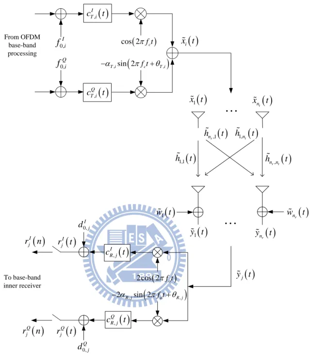
2.4: MIMO signal model with direct-conversion radio transceiver under the effects of I-Q imbalances, dc offsets, and frequency offset... 17

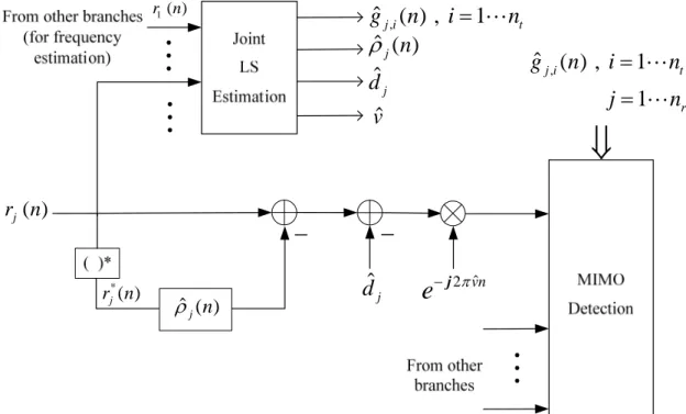
3.1: MIMO receiver with joint LS estimation/compensation of radio parameters. ... 22

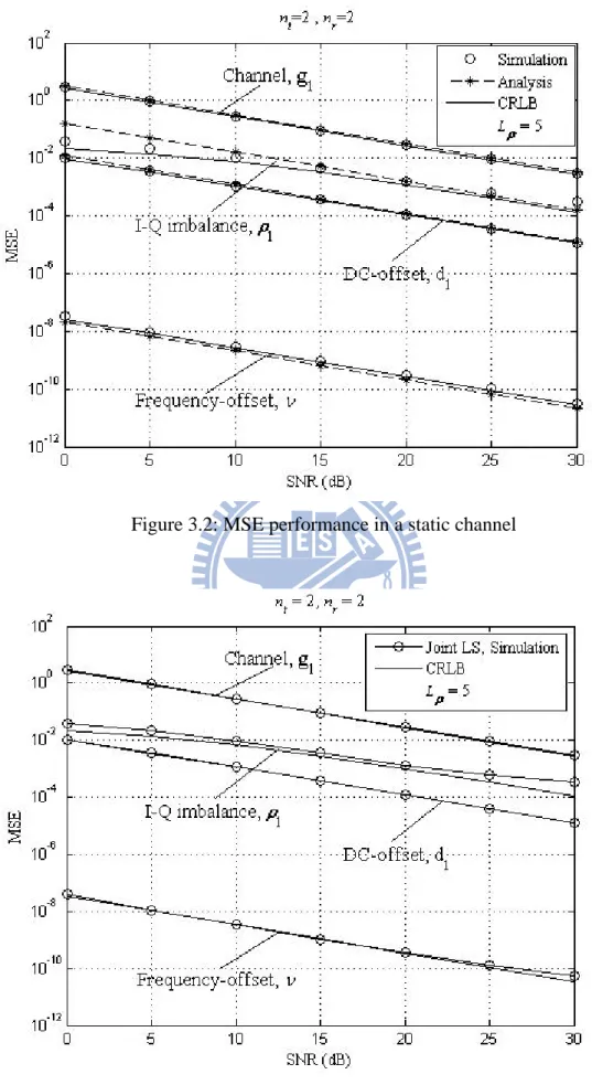
3.2: MSE performance in a static channel ... 47

3.3: MSE performance of the joint estimators in Rayleigh fading channels ... 47

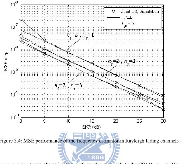
3.4: MSE performance of the frequency estimator in Rayleigh fading channels ... 48

3.5: The effects of L_ρ on MSE in Rayleigh fading channels... 49

3.6: The effects of L_ρ on BER performance in Rayleigh fading channels... 50

3.7: BER performance with low-complexity and/or simplified estimators in Rayleigh fading channels... 51

4.1: The two-stage cancellation architecture for cascaded transmitter and receiver radio impairments... 60

(12)

4.3: The two-stage cancellation architecture for transmitter radio impairments... 61 4.4: MSE performance comparison between JLSE and LCE-PT schemes... 71 4.5: Performance comparisons between the proposed methods, receiver radio compensation

only [63] and per-tone equalization (PTEQ) [48] (spatial-multiplexing MIMO-OFDM). .... 72 4.6: Performance comparisons between the proposed methods and Zou’s method [45] (STBC

MIMO-OFDM). ... 73 5.1: The calibration system consists of a direct-conversion RF transceiver, calibration circuits

and a joint estimator of the calibration parameters. ... 76 5.2: Performance of the calibrated E

[

IRR_T

]

with different L ’s under optimal training. ... 96 _f

5.3: Performance of the calibrated E

[

IRR_R

]

with different L ’s under optimal training. ... 96 _f

5.4: Performance of the calibrated E

[

IRR_T

]

with different training designs. ... 97 5.5: Performance of the calibrated E

[

IRR_R

]

with different training designs. ... 98 5.6: Empirical cumulative density functions of the calibrated IRR and _T IRR constructed _R

with 10 realizations. ... 99 6 5.7: Empirical cumulative density functions of the calibrated ε_T and ε_R constructed with

6

10 realizations. ... 99 5.8: Sample signal constellation with and without calibrations (σ₀2 = )...101 0 5.9: Bit error rate performance with and without calibration (64QAM)... 101

(13)

List of Tables

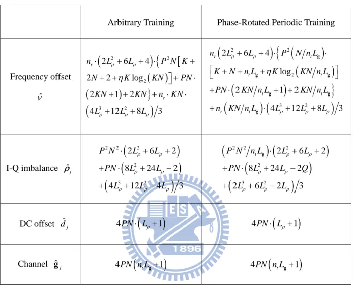
3.1: Computational Complexities of Arbitrary Training and Phase-Rotated Periodic Training

(Number of Real Multiplications)... 36

3.2: System Parameters and Radio Impairments... 45

4.1: Computational Complexities of JLSE and LCE-PT (Number of Real Multiplications) ... 69

4.2: System Parameters and Radio Impairments... 70

5.1: The RF impairments... 95

(14)

Notations

t

n : number of transmit antennas

r

n : number of receive antennas

j : -1

⊗: linear convolution operator ( )t

δ : Dirac delta function

( )

n

δ : Kronecker delta function *

( )⋅ : complex conjugate operator ( )⋅ : transpose of a matrix or vector T

( )⋅ : complex conjugate transpose of a matrix or vector H 1

( )⋅ : inverse of a square matrix −

( )⋅†: pseudo-inverse of a matrix or vector

[ ]

A i j, :

( )

i j, -thentry of matrix A ( )

(15)

det( )⋅ : determinant of a matrix

{ }

diag x : diagonal matrix with vector x on the diagonal

{

1

}

diag X ,…,X_M : block diagonal matrix with the submatrices X1,…,XM on the diagonal

E{}⋅ : expectation operator Re{}⋅ : real parts

Im{}⋅ : imaginary parts 10

log ( )⋅ : base-10 logarithm

N

1 : all 1 vector with dimension N

N

I : N×N identity matrix

N

0 : N×1 all zero vector

M N×

(16)

Chapter 1 Introduction

The demands for high-rate wireless communication services and cost-effective devices are getting stronger in recent years. On one hand, OFDM (orthogonal frequency-division multiplexing) equipped with multiple antennas at both transmitter and receiver has been devised as a key tech-nology to enabling high-rate, high spectral-efficiency wireless communications. OFDM is effec-tive in combating inter-symbol interference (ISI) in high-rate transmission [1] while using multi-ple transmit and receive antennas, also known as a multimulti-ple-input multimulti-ple-output (MIMO) tech-nology, is capable of providing diversity gain, array gain (power gain), and/or degree-of-freedom gain over the single-input single-output (SISO) systems [2]-[4]. MIMO-OFDM has been adopted in the IEEE 802.11n, IEEE 802.16, and 3GPP Long Term Evolution (LTE) specifications.

On the other hand, the direct-conversion radio architecture has been widely employed in to-day’s wireless devices [5]-[8]; without using intermediary frequency (IF) stages and the image rejection (IR) filter, it is more amenable to monolithic integration and, thus, facilitates a low cost, small form factor design. This architecture, however, is very sensitive to imperfections of the analog circuitry. In particular, mismatch between I and Q branch circuitry, called the in-phase/quadrature (I-Q) imbalance, induces mirror-frequency interference, and imperfection in

(17)

A/D and D/A converters and leakage from local oscillators induce dc offset. These radio fre-quency (RF) impairments, along with frefre-quency offset between transmitter and receiver, signifi-cantly degrade communication performance if not accurately compensated [9]-[65]. This is par-ticularly true in the next-generation high-rate systems, where wide bandwidth and high-order modulation are deemed to be employed. Furthermore, the radio impairments make the power am-plifier (PA) linearization circuit at the transmitter more difficult to work satisfactorily [50], [52], [56], and that may reduce the PA’s efficiency.

In this study, we are concerned with digital compensations of radio impairments in the wide-band MIMO systems with direct-conversion transceiver.

1.1 Estimation and Compensation Techniques of

Ra-dio Impairments

Removal and/or compensation of the radio impairments in the direct-conversion radio architec-ture have been an area of extensive research. Generally speaking, two types of technique have been proposed [9]-[61]: one is estimation/compensation and the other is self-calibration. The es-timation/compensation technique is to remove the impairments from the received signal during communication at the receiving side [9]-[49], whereas self-calibration is a technique to remove the transceiver’s own radio impairments before communication [50]-[61]. Both techniques find their applications in real systems [9]-[61], although self-calibration has the advantage to facilitate the design of the PA’s (power amplifier’s) linearization circuit. This dissertation will focus on both types of digital technique.

1.1.1 Estimation/Compensation Techniques

Quite a lot of works in the literature have been devoted to the radio impairments estimation and compensation for the direct-conversion architecture [9]-[49]. In [9]-[34], different methods were

(18)

developed to estimate and compensate the receiver radio impairments in SISO (single-input, sin-gle output) and MIMO (multiple input, multiple output) receivers. In [35]-[49], the cascaded transmitter and receiver radio impairments were investigated, with [35]-[40] focusing on the SI-SO systems and [41]-[49] on the MIMO systems. In the application configuration such as the downlink of a mobile cellular system, only the receiver radio impairments needed to be consid-ered because the transmitter impairments can be neglected due to the high-precision implementa-tion of the analog front-end in the base staimplementa-tion. For the applicaimplementa-tion configuraimplementa-tion of wireless peer-to-peer communication such as the wireless mesh networks, however, the cascaded effect of the transmitter and receiver radio impairments should be considered because it is very likely that a low-cost and, hence, a less precise analog front-end is implemented at both transmitter and re-ceiver. In the following, estimation/compensation techniques for different system configurations are discussed in more details.

1.1.2 Estimation/Compensation Techniques for Receiver Radio

Impairments

Various digital techniques have been developed for estimation and compensation of receiver radio impairments, which can be generally categorized into two types. One is the data-aided (DA) thods using known training sequences [16]-[34], and the other is the non-data-aided (NDA) me-thods exploiting some statistical properties of the received signal [9]-[15].

z Non-Data-Aided Techniques

In [9]-[15], adaptive or non-adaptive (block-based) statistical signal processing-based (blind) techniques were proposed for compensation of the receiver radio impairments. Blind source se-paration (BSS) techniques were introduced in [9]-[11] to cancel the self-image interference due to frequency-independent [9] and frequency-dependent [10][11] I-Q imbalance, respectively, based on the assumption that the desired signal and the image interference are statistically independent.

(19)

Such independence may be valid in the low-IF scheme but does not hold true in direct-conversion receivers. On the other hand, circularity-based compensation techniques were proposed in [12]-[15] based on the assumption that the desired signal is a complex random process with a circular-symmetric distribution. In [12]-[14], frequency-independent I-Q imbalance and/or dc offset were considered, while frequency-dependent I-Q imbalance was of interest in [15]. Con-vergence to the desired solution is not always guaranteed using blind approaches and no training data is needed at the expense of slow convergence rate.

z Data-Aided Techniques

In [16]-[20], dc offset was investigated under frequency offset, among which a low-complexity joint estimation was proposed in [20] based on periodicity of a training sequence. In [21][22], I-Q imbalances were investigated for OFDM (orthogonal frequency division multiplexing) systems in the absence of frequency offset and dc offset. In [21], I-Q imbalance was compensated by using a simple two-tap adaptive frequency-domain equalizer, while in [22], adaptive and non-adaptive post-FFT schemes were proposed for both frequency-dependent and independent I-Q imbalances at the receiver. In [24]-[29], I-Q imbalance was investigated jointly with frequency offset, with [24]-[26] focusing on frequency-independent I-Q imbalance and [27]-[29] on fre-quency-dependent I-Q imbalance. In [27]-[29], an FIR (finite impulse response) filter was pro-posed for compensating frequency-dependent I-Q imbalance and an asymmetric phase compen-sator for frequency-independent one. In particular, the periodic structure of a training sequence was exploited in [29] to develop a low-complexity estimation of I-Q imbalance and frequency offset. In [30], a joint least squares estimation of I-Q imbalance, dc offset and channel was pro-posed, and latter extended to [31], which developed a joint estimation of frequency offset, chan-nel, (frequency-independent) I-Q imbalance and dc offset in the time domain. Under the assump-tion of white Gaussian noise at the output of sampler, the ML (maximum likelihood) criterion was used in [31] to derive the solution. In [32], the pilot-based estimation and compensation of

(20)

I-Q imbalance were investigated for OFDM systems under timing offset and frequency offset. In [33], I-Q imbalance was investigated jointly with symbol detection for MIMO-OFDM sys-tems, with no consideration of frequency offset and dc offset. Using an extended channel model that incorporates I-Q imbalance, symbol detection was performed on the extended channel with-out explicit estimation/compensation of I-Q imbalance. Non-adaptive (e.g., least-squares) or adaptive (e.g., recursive least squares and least mean squares) filtering can be used for estimating the extended channel prior to symbol detection. Likewise, MIMO detectors such as ML, ZF (ze-ro-forcing), MMSE (minimum mean-squared error), etc. [4] can be employed for symbol detec-tion. Note that using the extended channel increases system dimension, and hence the detection complexity, as compared to the receiver in which RF impairments are estimated and compensated before the symbol detection.

1.1.3 Estimation/Compensation Techniques for Cascaded

Trans-mitter and Receiver Radio Impairments

Basically, two types of compensation for cascaded transmitter and receiver radio impairments have been investigated in the design of a digital receiver: one is cancellation based and the other is joint-detection based. In the cancellation type of techniques, radio impairments are estimated and cancelled explicitly from the received signal before a detection, which is designed with no consideration of radio impairments [35][36]. In the joint-detection type of technique, on the other hand, the detection and radio impairments compensation are performed jointly with no explicit estimation and cancellation of the radio impairments [37]-[49]. Due to the effect of mir-ror-frequency interference and inter-carrier interference, the dimension of signal detection in the joint-detection type of receiver is at least twice of that of the cancellation type, and that increases the detection complexity very significantly. This is especially true for the MIMO-OFDM (multi-ple-input, multiple-output, orthogonal frequency division multiplexing) systems, where MIMO detection has to be done for each sub-carrier.

(21)

For the MIMO-OFDM systems, which is a key enabling technology for high-rate wireless systems, the transmitter and receiver radio impairments were studied in [33],[34],[41]-[43], [45]-[49]. In particular, I-Q imbalances were investigated exclusively for the spatial-multiplexing systems in [33],[41]-[43] and for the space-time block coded (STBC) systems in [33][45][46]. In [47], the transmitter and receiver I-Q imbalances were investigated jointly with frequency offset for spatial-multiplexing and space-frequency block coded (SFBC) systems in a high mobility en-vironment. In [48][49], the authors proposed linear per-tone equalization (PTEQ) to the spa-tial-multiplexing and STBC systems in the presence of transmitter and receiver I-Q imbalances and frequency offset. The PTEQ method, nevertheless, is only applicable to a linear MIMO de-tection and suffers from a slow convergence. In all these works, the joint-dede-tection type of re-ceiver design was investigated exclusively. In [34], a cancellation type of MIMO-OFDM rere-ceiver was proposed, but only receiver frequency-independent I-Q imbalance and frequency offset were considered.

1.1.4 Calibration Techniques

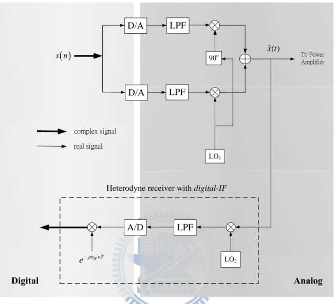
Many interesting works have been devoted to self-calibration of the radio impairments in the di-rect-conversion architecture [50]-[61]. In [50]-[53], adaptive methods were proposed to calibrate transmitter frequency-independent I-Q imbalance and dc offset by using an envelope-detector (ED) in the feedback loop. Transmitter frequency-dependent I-Q imbalance was calibrated for the continuous frequency-shift-keying (CFSK) systems in [54], with no consideration on other im-pairments. Frequency-dependent I-Q imbalance is particularly problematic in a wideband system, where the I-branch and Q-branch analog filters are difficult to be kept perfectly matched over the entire band. The works in [55]-[58] discussed calibration of transmitter frequency-independent and dependent I-Q imbalances by using a digital low-IF architecture in the feedback loop, as shown in Figure 1.1. And in [59], transmitter frequency-independent I-Q imbalance was cali-brated by using same reference signal at both transmit and receive paths.

(22)

Analog LPF ( ) x t

( )

s n complex signal real signal To Power Amplifier LPF D/A D/A 90o LO1 LO2 LPF A/D IF j nT e−ω Digital

Heterodyne receiver with digital-IF

Figure 1.1: Calibration feedback loop using heterodyne receiver with digital-IF

So far, most self-calibration techniques in the literature have been focused on the transmitter radio impairments, either by employing an ED [50]-[53] or a digital low-IF radio architecture [55]-[58] in the feedback loop so that the receiver impairments can be safely neglected. However, using ED or low-IF radio architecture in the feedback loop increases the hardware complexity. Besides, the calibration of the receiver impairments is important in its own right. For example, if one’s own receiver has been calibrated before communication, only the transmitter impairments (of the transmitting device), rather than the cascaded effect of the transmitter and receiver im-pairments, need to be estimated and compensated for at the receiver, and that reduces the receiver complexity. Very recently, the issue of joint self-calibration of transmitter and receiver radio

(23)

im-pairments was investigated in [60] and [61]. In [60], a two-feedback method was proposed, where the phase of the receive oscillator is shifted by exact 90 degrees in the second feedback, aiming to separate transmitter and receiver I-Q imbalances. Unfortunately, it is very difficult for analog circuitry to have an exact 90 degrees phase rotation in real systems. In [61], a new method was proposed for OFDM (orthogonal frequency-division multiplexing) type of systems with no dedi-cated analog circuit in the feedback loop. The method, however, can only calibrate the fre-quency-independent I-Q imbalance and dc offset.

1.2 Dissertation Outline and Contributions

This dissertation focuses on study and development of both types of estimation and compensation techniques of radio impairments for different MIMO communication application configurations, where the estimation/compensation techniques are investigated in Chapter 3 and Chapter 4 and the calibration technique in Chapter 5. In particular, Chapter 3 focuses on estima-tion/compensation technique of receiver radio impairments for the application configuration such as the downlink of a mobile cellular system, and then Chapter 4 extends to estima-tion/compensation technique of cascaded transmitter and receiver radio impairments for the ap-plication configurations such as the wireless peer-to-peer communication and the uplink of a mo-bile cellular system. The rest of this dissertation is organized as follows.

In Chapter 2, first, we describe the direct-conversion transceiver model including fre-quency-independent and frequency-dependent I-Q imbalances and dc offset. Then, three basic types of MIMO signal model that incorporates the transmitter and/or receiver radio impairments are introduced, which are related with different application configurations.

In Chapter 3, we propose to do joint estimation of frequency, receiver dc offset, receiver I-Q imbalance, and channel in MIMO receivers for improving its performance. Firstly, a receiver ar-chitecture that facilitates joint estimation and compensation of frequency, receiver dc offset,

(24)

re-ceiver I-Q imbalance and channel is proposed; both frequency-dependent and fre-quency-independent I-Q imbalances are included. Secondly, the LS criterion is applied to obtain the joint estimators, with a special training-sequence design to reduce complexity. Simplified es-timators on frequency and dc offset are also proposed with almost no loss in performance. Lastly, the LS estimators are shown through analysis to be un-biased and approach to CRLB (Cramér-Rao lower bound) for signal-to-noise ratios (SNRs) of interest. The results of this chap-ter have been published in [62] and [63].

In Chapter 4, the cancellation technique of cascaded transmitter and receiver radio impair-ments is investigated for the MIMO-OFDM systems with direct conversion radio architecture. A two-stage generalized cancellation architecture is proposed, where in the first stage, the receiver radio impairments such as frequency-independent and dependent I-Q imbalances and dc offset are cancelled along with frequency offset and transmitter dc offset in the time domain, and in the second stage, the transmitter frequency-independent and dependent I-Q imbalances are cancelled in the frequency domain. The two-stage cancellation architecture generalizes the cancellation ar-chitectures for transmitter and/or receiver radio impairments. Moreover, the technique is unique in that it is effective in different forms of MIMO operations including spatial multiplexing, STBC (space-time block coded) and transmit beam forming, with any number of transmit and receive antennas.In addition, two methods of radio parameters estimation are proposed. The first is the optimum joint least-squares estimation of channel and radio impairments which can be seen as an extension of Chapter 3. The second is a low-complexity iterative estimation that exploits the pe-riodic structure of a training sequence. The proposed methods are simulated and compared with existing methods. Simulation results confirm the superiority of the proposed methods. The results of this chapter have been presented partly in [64] and [65] and submitted as the journal paper [66].

In Chapter 5, a new self-calibration method is proposed which enables to self-calibrate the own transmitter and receiver radio impairments simultaneously, with no dedicated analog circuit

(25)

in the feedback loop. A frequency offset between transmitter and receiver is introduced purposely so as to separate the transmitter impairments from those of the receiver during calibration. Based on a time-domain approach, the new method is applicable to all types of communication systems and is able to calibrate jointly the frequency-independent I-Q imbalance, frequency-dependent I-Q imbalance, and dc offset. In addition, optimal training sequences are devised to best the cali-bration performance. The calicali-bration performance is analyzed that agrees very well with the si-mulations. Simulation and analytical results confirm the effectiveness of the proposed method. The results of this chapter will be presented partly in [67] and submitted as the journal paper [68].

Finally, Chapter 6 concludes the dissertation and discusses some possible extensions and top-ics for future research.

(26)

Chapter 2 System Models

In this chapter, direct-conversion transceiver model including frequency-independent and fre-quency-dependent I-Q imbalances and dc offset are described in Section 2.1. Then, three basic types of MIMO signal model that incorporates the transmitter and/or receiver radio impairments are given in Section 2.2, which are corresponding to different application configurations.

2.1 Direct-Conversion Transceiver Model

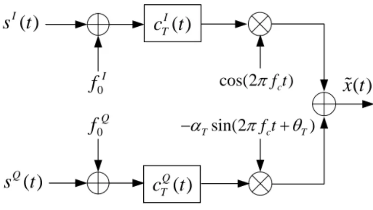
Figure 2.1 shows a mathematical model of a direct-conversion transmitter with I-Q imbalance and dc offset effects. Define s t

( )

=sI

( )

t + jsQ

( )

t be the baseband signal appearing at the input of transmitter. _0, _0,I _0,Q

i i i

f = f + jf characterizes the dc offset, which is due mainly to the imperfec-tion of D/A converters. The transmit analog filter effect of I and Q branch is modeled by c t_TI( ) and ( )c_TQ t with unit power, if c t_TI( )≠c_TQ( )t , it is said that there is a frequency-dependent I-Q imbalance. Taking into account the transmitter frequency-independent I-Q imbalance, the com-plex sinusoidal signal coming into the mixer is

2 2

( ) cos(2 ) sin(2 ) f tc f tc

T c T c T T T

(27)

cos(2π f tc ) sin(2 ) T f tc T α π θ − +

( )

Q

s

t

Q

_{( )}

T

c

t

( )

I

s t

c t

_TI

( )

x t

0 I

f

0 Q

f

Figure 2.1: Mathematical model of a direct-conversion transmitter with I-Q imbalance and dc offset.

where α_T and θ_T are the gain and phase imbalances due to the imperfect analog circuitry of the mixer, respectively, 1 2 1

(

T

)

T Te θ γ = +α j and 1 2 1

(

T

)

T Te θ ϕ ₌ ₋α −j

characterize the corre-sponding transmitter frequency-independent I-Q imbalance effect, and f is the center fre-_c

quency. Ideally, the complex sinusoidal C t should contain only the positive frequency, i.e. _T( ) 2

( ) f tc

T

C t =ej π . However, due to the gain and phase mismatches α_T and θ_T, there is a negative frequency component _e− j2πf tc _{with a magnitude of}

T

ϕ , which, along with frequency-dependent I-Q imbalance, cause interfering images in the transmitted signal. After up-conversion, the pass-band transmitted signal including overall transmitter radio impairments effect is

( )

{

( )

2

}

Re f tc

i i

x t = x t ej π with its equivalent base-band signal :

( )

( ) ( )

( )

*

( )

1 T T x t =c ₊ t ⊗s t +c ₋ t ⊗s t + f , (2.1) where

( )

1

(

( )

)

2 T I Q T T T T c _± t = c t ±α ejθ c t , (2.2) and

( )

*

( )

1 0 T 0 T f = f ⊗c ₊ t + f ⊗c ₋ t , (2.3) is the equivalent transmit dc offset. In (2.1), s t

( )

can be viewed as being transmitted by two

(28)

2cos(2π f t_o ) 2α_Rsin(2π f t_o θ_R) − + ( ) y t 0 Q d ( ) I R c t ( ) Q R c t 0 I d ( ) I r t ( ) Q r t ( ) I r n ( ) Q r n

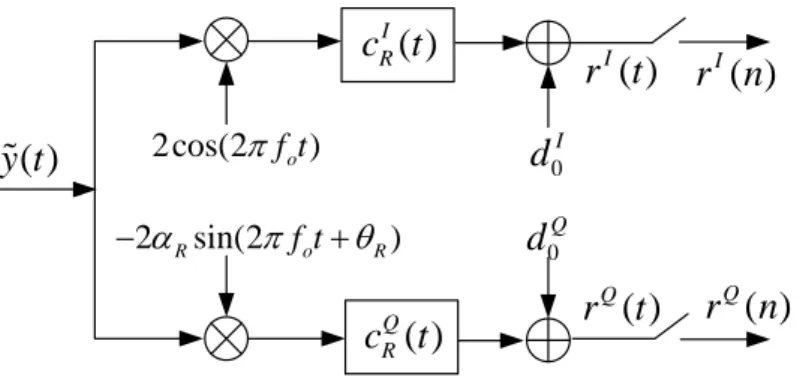
Figure 2.2: Mathematical model of a direct-conversion receiver with I-Q imbalance and dc offset.

channels with a corruption from dc offset; one is the desired channel with impulse response

( )

T

c ₊ t , and the other is the mirror-frequency channel with impulse response c_T₋

( )

t . That is, I-Q imbalances incur mirror-frequency interference in the transmitted signal, and dc offset, on the other hand, imposes a more strict specification on A/D converters at the receiver and may incur in-band interference in the presence of frequency offset. Note that with c_TI

( )

t =c_TQ

( )

t =c_T

( )

t , (2.2) degenerates to the case of no frequency-dependent I-Q imbalance with c_T₊

( )

t =γ_{T T}c

( )

t

and c_T₋

( )

t =ϕ_{T T}c

( )

t . In addition, with no I-Q imbalances and dc offset, i.e.,

( )

I Q

T T T

c t =c t =c t , 1α_T = and θ_T = f₀ = , 0 x t

( ) ( )

=s t ⊗c_T

( )

t , as one might expect. Similar to the direct-conversion transmitter, the mathematical model of a direct-conversion receiver with I-Q imbalance and dc offset is shown in Figure 2.2. Taking into account the fre-quency-independent I-Q imbalance at the RF front-end, the complex sinusoidal signal coming into the mixer is

2 2

( ) 2 cos(2 ) 2 sin(2 ) f tc f tc

R c R c R R R

C t = πf t − j α π f t+θ =γ e−j π +ϕ ej π ,

where α_R and θ_R are the gain and phase imbalances, respectively,

(

1 R

)

R Re θ γ _{= +}α −j , and

(

1 R

)

R Re θ ϕ = −α j

. After down conversion, c t and _RI( ) cQ_R( )t are the base-band filters used to

remove out-of-band noise and high-frequency components. Again, it is said to have a fre-quency-dependent I-Q imbalance if c t_RI( )≠c tQ_R( ). Frequency-dependent I-Q imbalance is mostly encountered in a wide-band RF receiver because it is generally difficult to maintain base-band

(29)

filters to have the same response over a wide frequency range. d_0,_j =d_0,I_j + jd_0,Q_j is the dc offset which is due to the imperfection of A/D converters and the self-mixing at the receiver’s mixer. After sampling, the end-to-end equivalent discrete system can be modeled as (up to a constant for the case of no aliasing)

( )

*

( )

0 I Q R R r n =r n + jr n =c ₊ n ⊗y n +c ₋ n ⊗y n +d , (2.4) where

( )

1

(

( )

)

2 R I Q R R R R c _± n = c n ±α e∓ jθ c n . (2.5) Again, (2.4) says that the receiver I-Q imbalances induces mirror-frequency interference in the received signal. With I

( )

Q

( )

R R R

c n =c n =c n , (2.5) degenerates to the case of no fre-quency-dependent I-Q imbalance with c_R₊

( )

n =1 2⋅γ_{R R}c

( )

n , and c_R₋

( )

n =1 2⋅ϕ_{R R}c

( )

n . In addition, if α_R =1, 0θ_R =d₀ = and I

( )

Q

( )

R R R

c n =c n =c n , we have the no I-Q imbalance and dc offset case; that is r n

( )

=c_R

( )

n ⊗y n

( )

.

2.2 System Models

The radio impairments may appear in transmitter and/or receiver, which depends on different system configurations. In the following, we address three kinds of system models corresponding to different application configurations, and the associated estimation/compensation techniques will be investigated in Chapter 3 and Chapter 4.

2.2.1 MIMO Systems under Receiver Radio Impairments

In this section, we address the MIMO system model that incorporates the receiver radio impair-ments, which is corresponding to the application configuration such as the downlink of the mo-bile cellular system.

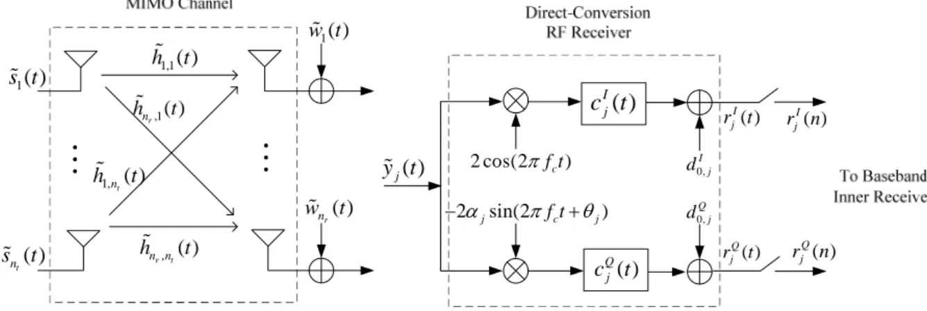
The MIMO signal model with a direct-conversion receiver is depicted in Figure 2.3. Consider a block transmission with a prefix to avoid inter-block interference. The pass-band transmit signal

(30)

2 cos(2πf tc) 2αjsin(2πf tc θj) − + ( ) j y t 0, Q j d ( ) I j c t , ( ) r t n n h t 1( ) s t ( ) t n s t 1,nt( ) h t ,1( ) r n h t 1,1( ) h t ( ) r n w t 1( ) w t ( ) Q j c t 0, I j d ( ) I j r t ( ) Q j r t ( ) I j r n ( ) Q j r n

Figure 2.3: MIMO signal model with direct-conversion RF receiver.

from i-th transmit antenna is

( )

Re

{

( )

2 f tc

}

i i

s t = s t ej π , with the base-band signal

( )

1 ,

( )

(

)

g N i i k T g s k n N s t s n g t k N N n T − =− =

∑ ∑

− + + , (2.6)

where f is the carrier frequency, _c si k,

( )

n is the transmitted k–th block symbols with the trans-mit power

( )

1 2 2 , 1 0 1 nt N s i k i n s n N σ − = =

=

∑∑

, N is the length of prefix, g N is the length of useful data,

( )

T

g t is the transmit filter with unit power, and T is the symbol time. _s

Let hj i,( )t =Re

{

h_{j i}_,

( )

t ej2πf tc

}

denote the channel response from i-th transmit to j-th receive antenna, and h_{j i}_,

( )

t be its base-band equivalent. The band-pass signal received from j-th

an-tenna is ( )

{

2

}

( ) Re ( ) fc f t ( ) j j j y t = y t ej π +Δ +w t , (2.7) where

( )

,

( )

1 ( ) t n j i j i i y t s t h t = =

∑

⊗ , (2.8)

{

2

}

0, ( ) Re ( ) f tc j j

w t = w t ej π is the pass-band additive white Gaussian noise and w_0,_j( )t is its

(31)

At the 'j th receiver side, α_j and θ_j are the frequency-independent gain and phase im-balances, respectively, c tI_j( )+ jcQ_j ( )t is the (unit-energy) base-band filter, and d_0,_j =d_0,I _j+ jd_0,Q_j

is the dc offset. Note that the radio parameters of I-Q imbalances and dc offsets are different from one branch to another. From (2.4), the end-to-end equivalent discrete system can be modeled as (up to a constant for the case of no aliasing)

r n_j

( )

=c₊_,_j

( )

n ⊗_⎣⎡y_j

( )

n ej2πνn+w_0,_j

( )

n _⎦⎤+c₋_,_j

( )

n ⊗⎡_⎣y_j

( )

n ej2πνn+w_0,_j

( )

n ⎤_⎦*+d_0,_j, (2.9) where _, ( ) 1 2 I( ) Q( ) j

j j j j

c_± n = ⋅_⎣⎡c n ±c nα e∓ jθ ⎤_⎦ , ν = ΔfT_S is the normalized frequency offset,

( )

,

( )

1 ( ) t n j i j i i y n s n h n =

=

∑

⊗ , and w_{0, j}

( )

n is a zero mean additive white Gaussian noise with

( )

2 2 0, E , 1 w w j n j nr σ ⎡_⎢ ⎤_⎥ =

⎣ ⎦ . In Chapter 3, we will investigate the estimation/compensation technique for receiver radio impairments.

2.2.2 MIMO-OFDM Systems under Cascaded Transmitter

and Receiver Radio Impairments

In this section, we address the MIMO-OFDM system model that incorporates the cascaded transmitter and receiver radio impairments, which is corresponding to the application configura-tion of wireless peer-to-peer communicaconfigura-tion such as the wireless mesh networks.

Figure 2.4 depicts a MIMO-OFDM system that employs a direct-conversion radio transceiver as the analog front-end subsystem. The base-band data signal for transmit antenna i is

( )

1 ,

( )

(

( )

)

g N I Q i i i i k g k m N s n s n s n s mδ n k N N m − =− = + j =

∑ ∑

− + − , (2.10) where

( )

1

( )

2 , , 0 1 N ml N i k i k l s m S l e N π − = =

∑

j (2.11)

(32)

(

)

cos 2π f t_c

(

)

, sin 2 , T i f tc T i α π θ − +

( )

, Q T i c t

( )

, I T i c t

( )

i x t 0, I i

f

0, Q i

f

( )

, r t n n h t

( )

1 x t

( )

t n x t

( )

1,nt h t

( )

,1 r n h t

( )

1,1 h t

( )

1 w t

(

)

2cos 2πf to

(

)

, , 2α_{R j}sin 2πf t_o θ_{R j} − +

( )

j y t 0, I j d

( )

, Q R j c t

( )

, I R j c t

( )

I j r t

( )

Q j r t

( )

I j r n

( )

Q j r n

( )

1 y t

( )

r n y t From OFDM base-band processing To base-band inner receiver 0, Q j d

( )

r n w t

Figure 2.4: MIMO signal model with direct-conversion radio transceiver under the effects of I-Q imbalances, dc offsets, and frequency offset.

is the inverse discrete Fourier transform (IDFT) of the transmitted data

{

_,

( )

}

1 0

N i k _l

S l ₌− in OFDM symbol k with the transmit power

( )

1 2 2 , 1 0 1 nt N s i k i m s m N σ − = =

(33)

and N is the FFT size. The cyclic prefix is assumed larger than the maximum delay spread of the overall channel consisting of the transmit filter, radio channel and receiver filter, and therefore there is no inter-OFDM symbols and inter-carrier interference.

At the i th' transmitter, _0, _0,I _0,Q i i i

f = f + jf characterizes the dc offset, and I_,( ) Q_,( )

T i T i

c t + jc t is the (unit-energy) base-band transmit filter. The frequency-independent I-Q imbalance is charac-terized by the parameters α_{T i}_, and θ_{T i}_,, which are the gain and phase imbalances respectively due to the imperfect analog circuitry of the mixer. f is the carrier frequency which is same for _c

all transmit antennas, ,( ) Re

{

_,

( )

2 c

}

f t j i _{j i}

h t = h t ej π is the channel response from transmit antenna

i to receive antenna j , and h_{j i}_,

( )

t is its equivalent base-band. ( ) Re

{

_0, ( ) 2 f to

}

j j

w t = w t ej π is

the pass-band additive white Gaussian noise, and w_0,_j( )t is its base-band equivalent.

At the j th receiver, ' α_{R j}_, and θ_{R j}_, are the frequency-independent gain and phase imbal-ances, respectively, cR jI_, ( )t + jcR jQ_, ( )t is the (unit-energy) base-band filter, and 0, 0, 0,

I Q j j j

d =d + jd

is the dc offset. f₀ = f_c− Δ is the local oscillator frequency of the receiver, where ff Δ is the

frequency offset between transmitter and receiver which is same for all receiver branches. From (2.1) and (2.4), the received discrete signal can be expressed as

( )

(

( )

₂

( )

)

( )

(

( )

₂

( )

)

* , 0, , 0, 0, , I Q j j j n n R j j j R j j j j r n r n r n c ₊ n y n e πν w n c ₋ n y n e πν w n d = + = ⊗ j + + ⊗ j + + j (2.12) where

( )

(

( )

*

( )

)

( )

, , 1, , 1 t n j i T i i T i i j i i y n s n c ₊ n s n c ₋ n f h n = =

∑

⊗ + ⊗ + ⊗ , (2.13)

( )

*

( )

1,i 0,i T ,i 0,i T ,i f = f ⊗c ₊ n + f ⊗c ₋ n , (2.14)

( )

(

( )

,

( )

)

, 1 2 , , , T i I Q T i T i T i T i c _± n = ⋅ c n ±α ejθ c n , (2.15)

(

,

)

, ,( ) 1 2 ( ) , , ( ) R j I Q R j R j R j R j c _± n = ⋅ c n ±α e∓ jθ c n , (2.16) s fT

(34)

Gaus-sian noise with σ_w2 E_⎢⎡w_0,_j

( )

n 2⎤_⎥, j=1 n_r

⎣ ⎦ .. We have used the notation,

( )

t nTs

x n x t ₌ for a signal x t

( )

, where T is the sampling period. _s

2.2.3 MIMO-OFDM Systems under Transmitter Radio

Im-pairments

For the application configuration such as uplink of mobile cellular system, the receiver radio im-pairments are negligible except for frequency offset due to the high-precision implementation of the analog front-end in the base station while the transmitter radio impairments needed to be con-sidered due to the mobile station with a less precise analog front-end. As a special case in Figure 2.4, there is no receiver I-Q imbalances and receiver dc offset, i.e. αR j, =1, 0θR j, =d0,j = and

( )

, , ,

I Q

R j R j R j

c n =c n =c n , 1,j= …,n_r. Hence, the received discrete signal model in (2.12) for a MIMO-OFDM system under transmitter radio impairments and frequency offset degenerates to

( )

(

( )

)

( )

(

( )

)

( )

2 , 0, 2 * , , , 1, , 0, 1 t n j R j j j n n R j i T i i T i i j i j i r n c n y n e w n c n e s n c n s n c n f h n w n πν πν + − = = ⊗ + ⎡ ⎤ = ⊗_⎢ ⊗ + ⊗ + ⊗ + _⎥ ⎣

∑

⎦ j j . (2.17) In Chapter 4, we will investigate the estimation/compensation technique for cascaded transmitter and receiver radio impairments.

(35)

Chapter 3 Estimation/Compensation

Technique for Receiver Radio

Impairments

In this chapter, the estimation/compensation technique of receiver radio impairments is investi-gated for applications such as downlink MIMO communications. A receiver architecture that fa-cilitates joint estimation and compensation of radio parameters is proposed in Section 3.1. The least squares (LS) criterion is then applied to obtain the joint estimators in Section 3.2, with a special phase-rotated periodic training-sequence design to reduce complexity. Simplified estima-tors on frequency and dc offset are also proposed with almost no loss in performance. The com-putational complexities and performances of proposed estimators are analyzed in Section 3.3 and Section 3.4, respectively. Simulation results are given in Section 3.5. Finally, Section 3.6 summa-rizes this chapter.

(36)

3.1 Receiver Architecture

We start from the received signal model (2.9) with receiver radio impairments effect in subsection 2.2.2. Motivated by (2.9), one way to process the received signal is to cancel out firstly the self-image interference due to I-Q imbalance. By introducing the filter ρ_j

( )

n , we have

( )

(

( )

)

(

( )

)

( )

(

)

(

( )

)

( )

(

)

* * 2 , , 0, * * 2 , , 0, 0 * 0, 0, ( ) ( ) . n j j j j j j j j n j j j j j j j j r n n r n c n n c n y n e w n c n n c n y n e w n d n d πν πν ρ ρ ρ ρ + − − + = − ⊗ = − ⊗ ⊗ + + − ⊗ ⊗ + + − ⊗ j j (3.1)

To completely cancel out the self-image interference, ρ_j

( )

n =

(

c₊*_,_j

( )

n

)

−1⊗c₋_,_j

( )

n , where

( )

(

_*

)

1

, j

c₊ n − is the inverse filter of c*₊_{, j}

( )

n . (For the case of no frequency-dependent I-Q imbal-ance, ρ_j

( )

n =ϕ γ_j *_j as is given in [31].) Thus, (3.1) becomes

( )

(

)

(

( )

)

( )

* * 2 * , , 0, 0, 0, 2 , 1 , j t j j j n j j j j j j j j c n n n i j i j j i r n n r n c n n c n y n e w n d n d e s n g n d w n πν πν ρ ρ ρ + − = = − ⊗ ⎡ ⎤ =_⎣ − ⊗ _⎦⊗ + + − ⊗ ⎛ ⎞ = _⎜ ⊗ _⎟+ + ⎝

∑

⎠ j j (3.2) where c_j

( )

n =c₊_,_j

( )

n −ρ_j

( )

n ⊗c₋*_,_j

( )

n , g_{j i}_,

( )

n h_{j i}_,

( )

n ⊗

(

c_j

( )

n e−j2πνn

)

, d_j =d_0,_j−ρ_j

( )

n ⊗ * 0, j

d , and w n_j

( )

=c_j

( )

n ⊗w_0,_j

( )

n . g_{j i}_,

( )

n is the overall impulse response from i-th transmit to

j-th receive antenna after canceling out the self-image interference, d is the dc offset, and _j

( )

j

w n is an additive Gaussian noise but generally not white. In (3.2), ρ_j

( )

n , g_{j i}_,

( )

n , ν , and

j

d are the deterministic, unknown parameters to be estimated. In what follows, ρ_j

( )

n and

( )

,

j i

g n will be approximated as FIR (finite impulse response) filters with large enough taps, al-though they are generally IIR (infinite impulse response) ones, as can be seen in (3.1).

(37)

ˆ ( )_j n ρ

d

ˆ

j ( ) j r n

−

ˆ 2 vn

e

− j π

ˆ ( )

_j

n

ρ

ˆ ( ) ,

j i,

1

t

g

n

i

=

n

ˆ

j

d

ˆ

v

* ( ) j r n

⇓

,

ˆ ( ) ,

1

j i t r

g

n

i

n

j

n

=

−

1( ) r n

Figure 3.1: MIMO receiver with joint LS estimation/compensation of radio parameters.

self-image interference, dc offset is compensated next, and then compensation for frequency off-set follows. The parameters ρ_j

( )

n , g_{j i}_,

( )

n , ν , and d will be estimated jointly in the least _j

squares sense, as to be discussed in the next section, and the MIMO detection is done with the MMSE detector, based on the estimated channel responses

{

gˆ_{j i}_,

( )

n

}

along with the compen-sated received signals from all branches. Some other types of MIMO detectors can be used as well [70].

3.2 Joint Least Squares Estimation

In this section, the set of radio parameters ρ_j

( )

n , g_{j i}_,

( )

n , ν , and d are estimated jointly in _j

the sense of least squares. In order to do that, ρ_j

( )

n and g_{j i}_,

( )

n are approximated by the FIR filters

( ) ( )

0 , 1 , ,

(

1

)

j T j =⎡⎣ρj ρj … ρj Lρ − ⎤⎦ ρ and

( )

(

)

, , , 0 , ,, 1 , , , j i 1 T j i =⎡⎣gj i gj i gj i Lg − ⎤⎦ g … with

(38)

the length

j

L_ρ and

,

j i

Lg , respectively. In the following, Lρ_j =Lρ, ∀j, and Lgj i, =Lg, ,∀i j. In

addition, L_ρ and L_g are assumed to be large enough (to contain 99% of the energy) in this and next sections, and thus approximation error is negligible. The impact of L_ρ and L_g will be in-vestigated by computer simulations in Section 3.4. For a data-aided estimation as considered here,

( )

,

i k

s n is known perfectly to the receiver. A total of P≥ training blocks will be assumed in 1 this paper, starting from the zero-th block

(

k=0

)

.

3.2.1 Least Squares Estimators

Consider the case of L_g ≤N_g ; thus there will be no inter-block interference. Let

( )

,

( )

0 , ,

( )

1 , , ,

(

1

)

T j k =⎡⎣rj k rj k rj k N− ⎤⎦

r … be the useful part of the k-th received block, where

( )

(

)

,

j k j g

r n r k N +N +n , Rj

( )

k be the N×Lρ received signal matrix with

( )

_, ,

(

)

j k _{m l} rj k m l

⎡ ⎤ = −

⎣R ⎦ , 0≤ ≤ −m N 1 , 0≤ ≤l L_ρ−1, and S_i

( )

k be the N×L_g signal matrix with

( )

_,

(

)

,

i k _{m l} =si k m l−

⎡ ⎤

⎣S ⎦ , 0≤ ≤ −m N 1 , 0≤ ≤l L_g−1. From (3.2), the useful part of the

j-th received signal can be written as the vector form

( )

*

( )

, 1 , 0, , 1, t n j j j k i j i j N j i k k ν k d k k P = ⎛ ⎞ − _⎜ _⎟+ + = − ⎝

∑

⎠ r R ρ =Γ S g 1 w … (3.3) where

( )

2 k N( g N v) diag 1, ,

{

2 v , 2 v N( 1)

}

k e e e π π π ν ₌ + _⋅ _⋅⋅⋅ − Γ j j j

is a diagonal matrix, and

( )

,

( )

0 , ,

( )

1 , , ,

(

1

)

T j k =⎡⎣wj k wj k wj k N− ⎤⎦ w … with w_{j k}_,

( )

n w k N_j

(

_g +N

)

+n

)

. Furthermore, define

( ) ( )

0 , 1 , ,

(

1

)

T T T T j =⎡⎣ j j j P− ⎤⎦ r r r … r ,

( )

0 ,

( )

1 , ,

(

1

)

T T T T j ⎡⎣ j j j P− ⎤⎦ R R R … R ,

寬頻多入多出直接轉換傳收機之射頻劣化效應估算與補償技術

國 立 交 通 大 學

電信工程研究所

博 士 論 文