行為財務學與行為會計學整合型計畫－子計畫二：以自願性 vs. 強制性財務預測作為公司治理之機制─理論與實驗證據

行政院國家科學委員會專題研究計畫 成果報告

子計畫二：以自願性 vs. 強制性財務預測作為公司治理之

機制─理論與實驗證據

中 華 民 國 93 年 12 月 13 日

Mandatory Earnings Forecasts, Legal Regime, and Auditor Independence

− Theory and Experimental Evidence

Hung-Chao Yu Department of Accounting

College of Commerce National Chengchi University

Wenshan, Taipei, 11605 TAIWAN, ROC

Rong-Ruey Duh Department of Accounting National Taiwan University

(02) 2363-0231 ext. 2977

1. INTRODUCTION

Independence requires the auditor to act with integrity and objectivity both in mental attitude and in appearance (Dopuch, King, and Schwartz 2003; SEC 2000). In operational term, independence ensures that the auditors be mentally objective in collecting, evaluating, and reporting on financial information. The Public Oversight Board’s Panel on Audit Effectiveness emphasizes that independence is “fundamental to the reliability of auditor’s reports.” (POB 2000, 109). Because auditor independence not only increases the likelihood that firms’ financial statements are in conformity with the generally accepted accounting principles (GAAP), but also encourages investors to rely more on the financial statements, it has long been regarded as a cornerstone to the public accounting profession (Mednick 1997; AICPA 1999; Levitt 2000; SEC 2000). However, since many recent audit failures have been attributed to a lack of independence (e.g., Arthur Andersen vs. Enron 2001; Ernst & Young vs. PeopleSoft 2003), a call to restore public confidence through improving auditors’ independence has been emphasized by regulators, accounting practitioners, and auditing academic (e.g., Abbott, Parker, Peters, and Raghunandan 2003; Citron 2003; Cote 2002; Craswell, Stokes, and Laughton 2002; Dopuch, King, and Schwartz 2003; Gerde and White 2003; Hodge 2003; Kaiser and Perris 2003; Kopel 2003; Lousteau and Reid 2003; SEC 2003).

Section 201 of the Sarbanes-Oxley Act of 2002 proposes one mechanism to enhance auditor’s independence: the prohibition of providing nonaudit services. Regulators’ concerns about nonaudit services are based on the assumption that auditors are willing to sacrifice their independence in exchange for retaining clients that pay large nonaudit service fees. Several recent studies use the newly available audit fee data and factors associated with earnings management or auditor’s propensity to issue going-concern reports to empirically examine whether nonaudit services adversely affect auditor independence (e.g., Ashbaugh, LaFond, and Mayhew 2003; Chung and Kallapur 2003; DeFond, Raghunandan, and Subramanyam 2002; Frankel, Johnson, and Nelson 2002; Whisenant,

Sankaraguruswamy, and Raghunandan 2003). The results, however, provide mixed support for the contention that nonaudit services do threaten auditor independence. In light of these and other anecdotal evidence, the efficacy of this proposed mechanism is still in debate. Therefore, more research should continue to explore and examine other mechanisms that may improve auditor independence for regulatory purposes.

In this study, we propose two mechanisms that may jointly improve auditor independence and induce firms’ truthful reporting and new investment: the legal regimes (negligence vs. strict) imposing on auditors and mandatory earnings forecasts made by managers. Prior analytical and experimental studies in auditor’s legal liability have compared the relative effectiveness of different legal regimes (Dopuch and King 1992; King and Schwartz 1999, 2000; Radhakrishnan 1999; Schwartz 1997) on audit effort and firm’s investments. However, few attempts, if any, have ever been made to investigate the effects of alternative legal regimes on auditor independence and firms’ honest reporting. Regarding the former, we posit that an appropriate legal regime should provide strong incentive for auditors to remain independent because doing otherwise auditors will be penalized by large damage compensation. Regarding the latter, extant research indicates that firms manage earnings to meet market expectations (e.g., Kasznik 1999; Nelson, Elliot and Tarpley 2002).

Kasznik (1999) empirically shows that managers use positive discretionary accruals to manage reported earnings upward when earnings would otherwise fall below management’s earnings forecasts. Thus, managers with a relatively greater ability to manage reported earnings could be less reluctant to release earnings forecasts, because they are better able to avoid the costs associated with forecast errors (e.g., legal exposure and management’s loss of reputation for forecast accuracy) without losing any of the potential benefits. This further implies that firms that are not willing to or less able to manage earnings may be reluctant to release earnings forecast due to the costs associated with not meeting the forecast. This could have two adverse consequences which may affect capital market’s reliance on

financial information. One is that management earnings forecast may be dominated by firms that release optimistic forecast. The other is that firms voluntarily releasing earnings forecast may not truthfully report earnings given that auditors do not deter their clients’ earnings management attempts. Since management earnings forecasts are made only voluntarily under the current U.S. practice, we posit that a mandatory earnings forecast (which requires firms to report earnings forecasts), together with an effective legal regime imposing on the auditor (which improves auditor independence and, in turn, mitigate managers’ earnings management), may jointly motivate managers of firms to report credibly because managers have to face the costs associated with the forecast errors. Since prior studies look at auditor’s legal regimes and management earnings forecasts in isolation, their results are limited and may not provide a sufficiently confirmatory foundation upon which to predict or describe auditor’s and manager’s optimal strategies and responses. In light of this deficiency, our study contributes to the literature by linking studies in auditor independence, auditor’s legal liability, and earnings forecasts to analytically and experimentally examine how different combinations of these two mechanisms may affect auditor independence and firms’ reporting and investment behavior.

Our study also extends the auditor’s liability literature that focuses on audit quality by separating audit failure into two types: a technical and an independence audit failure. This distinction is important for three reasons. First, the Enron scandal reveals the fact that an audit failure resulting from auditor’s compromising his independence may entail huge losses1 _{to the capital markets and deteriorate public} trust to the auditing profession that is much higher than an audit failure resulting from auditor’s imperfect audit technology or lower audit effort. Previous studies have generally assumed that the audit technology has one-sided error and defined audit failure as the probability that a firm with a high audited report is actually of low type (Dye 1993; Dye, Balachandran, and Magee 1990; Melumad and Thoman 1990; Hillegeist 1999; Pae and Yoo 2001; Schwartz 1997; Thoman 1996), but have often

1_{According to Business Week’s (1/28/2002) special report, the Enron debacle results in a $50 billion bankruptcy, $32} billion lost in market cap, and employee retirement accounts drained of more than $1 billion.

overlooked the possibility and existence of independence audit failure. Second, the Title II of the Sarbanes-Oxley Act of 2002 and the SEC’s 2003 final rules on auditor independence2 _{are more likely} to be concerned with the incidence of independence audit failure rather than with technical audit failure. Finally, since a technical audit failure represents an unknowing violation of the securities laws, the 1995 Reform Act rules that the auditor is held liable for damage losses proportionately.3 _{Therefore, the} auditor can minimize damage payments due to technical audit failure by varying his audit effort. In contrast, an independence audit failure involves a situation in which the auditor knowingly commits a violation of the securities laws. Consequently, the 1995 Reform Act requires that the auditor be held liable for the total damages jointly and severally. Note that a technical audit failure results from the imperfection of audit technology or a lack of due professional care, but an independence audit failure results from auditor’s intentionally compromising his independence. Without distinguishing between these two types of audit failure, prior studies in auditor’s legal liability could not fully examine the interactive effects among auditor’s effort level (which affects the technical audit failure), auditor’s independence decision (which affects the independence audit failure), and firm’s new investments under a setting that incorporates the salient features of the 1995 Reform Act.

We adopt the experimental economics methodology to address the issues of interest because of several reasons. First, there is a lack of naturally occurring data on important variables (in the real world, for instance, it is impossible to vary auditors’ liability levels and observe subsequent changes in firms’ new investments). Also, laboratory experiments provide a more precise measure of auditor independence than prior empirical-archival studies (e.g., the use of proxies such as the ratio of nonaudit service fees to audit fees or the magnitude of discretionary accruals). Second, because our

2_{On January 22, 2003, the SEC approved new rules intended to strengthen the independence of external auditors. The new} rule, entitled Strengthening the Commission's Requirements Regarding Auditor Independence, are mandated by Title II of the Sarbanes-Oxley Act of 2002, which requires the SEC to adopt by January 26, 2002, final rules under which certain nonaudit services are prohibited; conflict of interest standards are strengthened; auditor rotation requirements are enhanced, and reports by the auditors to audit committees will be expanded and clarified. The final rules can be found on the SEC’s Website at: http://www.sec.gov/rules/final/33-8183.htm.

model predicts multiple equilibria about manager’s and auditor’s strategic behavior, experimentation provides a useful means to explore actual behavior and equilibrium selection. Finally, it is impossible to vary the legal regimes in the real world and observe different players’ corresponding behavior. Therefore, the ability of empirical-archival research to offer policy insights is inherently limited (Kachelmeier and King 2002). Since the policy makers’ perspective demands ex ante insights of manager’s and auditor’s likely responses to different combinations of legal regimes and earnings forecast enforcement that could exist, laboratory experiments provide a controlled environment to address auditor independence and manager’s truthful reporting issues that may bear policy implications.

The remainder of this report is organized as follows. Section 2 presents the model setting, different players’ strategic behaviors, and hypotheses. Section 3 describes the experimental design, the procedures, and the methods.

2. BASIC MODEL AND HYPOTHESIS DEVELOPMENT 2.1 Basic Model Setting:

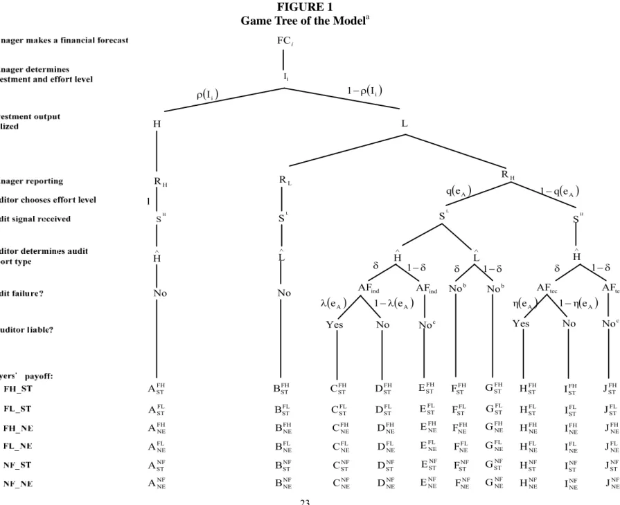
This study develops a one-period two-player game theoretic model in which there is one limited-liability manager who needs to raise fund from outside investor and one auditor who attests the realized earnings information disclosed by the manager. The manager first makes an earnings forecast, which can be either high (denoted by FChigh) or low (denoted by FClow). To achieve this targeted earnings level, the manager has to undertake an investment project (whose amount will influence the realized earnings). Since the firm has no internal funds, the manager must raise the money from an outside investor. The scale of the expansion is flexible and can be adjusted to the amount of the investment I (Table 1 shows definitions of the variables and parameter values for the illustrative example; Figure 1 demonstrates the game tree). To simplify the model setting, we assume that the investors are willing to provide I to the firm for carrying out the expansion. After obtaining the

money, however, the manager may choose to invest the whole amount of I on a high-cost innovative project (denoted by I_high) or only invest part of I on a low-cost established project (denoted by I ) _low

because the manager needs to exert a corresponding effort level i M

e (where i ∈ {high, low}) at an effort cost ( i )

M

e

C . The realized earnings ω is private information to the manager and can be either H

or L, depending on the dollar amount invested. Given the investment amount Ii , we define ρ(I_i) to be the probability that the outcome is H, where ρ(Ii) is increasing in Ii and ρ(Ii)∈ (0, 1). In the

numerical example, if Ilow is undertaken, the manager has a 0.80 probability of receiving L and a 0.20 probability of receiving H (i.e.,ρ(I_low) = 0.2). In contrast, if Ihigh is undertaken, the manager

would have a 0.80 probability of receiving H and a 0.20 probability of receiving L (i.e.,ρ(I_high) = 0.8). To be responsible for the investors who provide the funds, the manager prepares a financial report Rk,

where k∈{H,L}, and pays a flat audit fee F to hire a risk-neutral independent auditor to verify the credibility of his report Rk.4 We assume that, if the actual outcome is H, the manager will always

report RH. In contrast, if the actual outcome is L, the manager may report RH or RL. The auditor

chooses an effort level eA at a cost C(e_A)and obtains an audit signal ξ regarding the probable outcome of the earnings level. Let SH (or SL) denote the audit signal that the earnings level is high (or low), ξ∈ {SH, SL}.

[Insert Table 1 and Figure 1 here]

4_{The use of flat audit fees can be justified by several reasons. First, this setting is consistent with the rules that prohibit} contingent fees. Therefore, if the investors suffer losses due to misstatements in the financial statements, their only remedy is to sue the auditors for compensation. Second, instead of incorporating a formal bidding process, a flat audit fee can simplify the experimental setting for the subjects. This also allows my model to focus cleanly on auditor’s effort and reporting strategies without introducing undue complexity to the environment. Finally, Simunic and Stein (1996) finds that upward adjustment of audit fees is “made almost exclusively through higher levels of auditor effort, rather than through a pure price premium.” (p.120). This finding contradicts with the general belief that the auditor will raise audit fee to cover the increased auditing and litigation costs. In fact, high competition in the public accounting profession and price elastic demand arising from an excess supply of audits may prevent CPA firms from simply raising their audit fees to cover the potential litigation risk. This is consistent with Hillegeist’s (1999) argument that the audit fee is fixed in the U.S. current audit environment.

Since the audit technology is imperfect, there is no audit evidence from which the auditor can infer the investment outcome with certainty. Following Schwartz (1997) and Hillegeist (1999), we assume that the audit technology has one-sided errors: If the true outcome is H, the auditor will not obtain SL (i.e., p(SH |H) = 1), no matter what effort level the auditor exerts. If the true output is L, however, the auditor will obtain a correct signal SL with probability q(eA) and obtain an incorrect signal SH _{with probability 1 ( )}

A

e q

− . Consistent with Schwartz (1997), this q(eA) serves as a measure of audit quality, which is increasing in auditor’s effort level. For simplicity and tractability purposes, we assume that the auditor has two effort level to choose: a low effort level (denoted by low

A

e )

or a high effort level (denoted by high A

e ). In the numerical example, if the true outcome is H, the auditor will always obtain signal SH with probability one. If the true outcome is L, on the other hand, the auditor will obtain signal SL with probability 0.7 if he exerts high

A

e (i.e., ( high)=0.7)

A

e

q but will

obtain the correct signal with probability 0.3 if he only exerts low A

e (i.e., ( low)=0.3)

A

e

q .

Based on the manager’s report R and audit signal obtained, the auditor issues an audit report r ∈ { Hˆ , Lˆ } to the investors. To provide the manager with strong impetus to induce the auditor to issue a favorable audit report, we follow Dopuch et al. (2001) by assuming that the auditor’s report affects manager’s compensation: An Hˆ report results in a higher compensation for the manager than an Lˆ

report (denoted by M_Hˆ and M_Lˆ, respectively). Since this study focuses on auditor’s independence and manager’s reporting behavior, a more detailed discussion of their reporting strategies are given below. First, if the realized earnings level is H, the manager will always report RH (i.e., the manager’s reporting strategy is such that p(RH |H)=1). In this situation, the auditor will always obtain an audit signal SH and can only issue an Hˆ report (i.e., the auditor’s reporting strategy is such that

1 ) | ˆ ( H = S H

p ). This setting is consistent with current auditing practice in which the auditor will issue an unqualified opinion when audit evidence shows that there is no material misstatement in client’s

financial statements. If the realized earnings level turns out to be L, however, the manager can report

either RH or RL, depending on his financial reporting decision. After observing manager’s RL report,

the auditor believes that the true outcome is L and will issue an Lˆ report. If the manager reports RH, on the other hand, the auditor may obtain an SH signal from two possible scenarios: (a) the true outcome is L and the auditor has 0.3 probability of obtaining SH when he exerts high

A

e , and (b) the true outcome is L and the auditor has 0.7 probability of obtaining SH _{when he exerts} low

A

e . I refer to these

two scenarios as a technical audit failure (denoted by AFtec) because the auditor cannot effectively discover the true outcome of the earnings due to his imperfect audit technology and effort level. Therefore, the AFtec rate can be defined as the conditional probability that the auditor receives an RH

report from the manager and obtains an audit signal SH when the realized earnings level is L (i.e., AFtec

≡ _p(_L|_SH,_RH)_{≡ p}(_RH |_L)(1_−ρ(_Ii))(1_−q(_eA))/[_ρ(_Ii)_+p(_RH |_L)(1_−ρ(_Ii))(1_−q(_eA))]_{). Apparently,}

this AFtec rate is decreasing in auditor’s effort eA and manager’s investment level I, ceteris paribus.

When an AFtec occurs, the auditor’s legal liability will depend on the state of the economy and the

auditor’s effort level. In particular, if the state of the economy is good (with probability 1−δ), we assume that the firm will not go bankrupt (even though the earnings level is L) and, therefore, the

investors will not sue the auditor for damage compensations. In contrast, a lawsuit against the auditor will be triggered when the state of the economy is bad (with probability δ) because the firm cannot survive as a going-concern due to its low earnings level. During its deliberations, the court compares its own (noisy) observation of the audit’s quality to its interpretation of the legally required “due care” level of audit quality in determining whether to hold the auditor liable for AFtec. We assume that, in

expectation, the court will find the auditor negligent with probability η(eA), where η(eA) is

decreasing in auditor’s effort level. In the numerical example, the auditor has 0.3 (or 0.7) probability of being held liable if he exerts high

A

e (or low A

this )η(e_A is manipulated to be less than one (either 0.3 or 0.7) under the negligence legal regime (denoted by NE) and equal one under the strict legal regime (denoted by ST) to reflect the fundamental difference between these two legal regimes. If the court holds the auditor liable, the auditor has to pay a total damages D to the investors. Following Schwartz (1997), the damages D_tec tec are set to be independent of the actual investment Ii.

Alternatively, if the manager report RH but the auditor obtains a low signal SL, the imperfect audit

technology ensures the auditor that the true earnings is L. In this situation, the auditor may issue either an Hˆ or Lˆ report, depending on his independence decision. Since the manager’s compensation is

influenced by auditor’s report, the manager has strong motivation to induce the auditor to issue an Hˆ

report. To create a setting in which the auditor will compromise his independence to the highest level, I assume that the manager provides two incentives to the auditor: one is the present value of quasi rents accrued in future audit engagements (DeAngelo 1981), denoted by ER, and the other one is manager’s

side payment to the auditor in the current period (Lee and Gu 1998), denoted by SP. Under this setting, the

auditor has two reporting strategies to choose. If he intends to keep ER and accepts the SP, the auditor will

issue an Hˆ report. I refer to this scenario as an independence audit failure (denoted by AFind) because

the auditor intentionally misrepresents the true outcome of the earnings due to his lack of independence. The AFind rate is thus equal to the conditional probability that the auditor issues an Hˆ report when the

manager reports RH and the audit signal is SL (i.e., AFind ≡ ( ˆ | , H)

L _R

S H

p ). When an AFind occurs, the

auditor’s legal liability will still depend on the state of the economy and his effort level. If the state of the economy turns out to be good, the investors will not sue the auditor for damage losses because the firm is not bankrupt. In contrast, the investors will file a lawsuit against the auditor when the state of the economy is bad because the firm will go bankrupt. Since the auditor commits a knowing violation of the securities laws, the 1995 Reform Act rules that he will be held liable for the AFind damages jointly and severally.

Again, we assume that, in expectation, the court will find the auditor negligent with probability λ(e_A). If the court holds the auditor liable, it then determines the total damages D (which is also set to be _ind

independent of the actual investment Ii) the auditor should pay to the investors.

If the auditor refuses the SP and insists on issuing an Lˆ report (i.e., the auditor is independent or_p(_Lˆ|_SL,_RH)=1_{), the manager will incur an adjusting cost AC to modify his report R and will replace} the auditor at a switching cost (denoted by SC) and . Because the auditor is dismissed, he will lose the present value of future quasi rents ER. This one-period game then ends. Note that the manager will incur a cost low

high

C (or benefit high high

B ) if his earnings forecast is FChigh but the audited earnings report is RL (or RH).

Similarly, the manager will sustain a cost low low

C (or high low

C ) if his earnings forecast is FClow but the audited

earnings report is RL (or RH). Appendix 1 summarizes different players’ payoffs under different

combinations of earnings forecast enforcement and legal regimes. 2.2 Players’ Equilibrium Strategies and Hypotheses:

The analysis of the above game proceeds by backward induction because of the game’s sequential nature. However, the complexity of the model and the legion of endogenized variables introduce ambiguity into the analytical results due to some “high order” effects that may attenuate the comparisons and intuition among different legal systems. I overcome this problem by solving the game using the parameter values specified in Table 1. Table 2 summarizes the manager’s and auditor’s equilibrium strategies and payoffs under different legal systems.

[Insert Table 2 here]

As depicted in Table 2, when earnings forecasts are mandated, there are two competing equilibria for each of the two legal regimes. For example, columns (B) and (C) predict that the manager will make FChigh, undertake Ihigh, and always report RL when the realized earnings level is L. The auditor

will respond to these strategies by exerting low A

SL, resulting in an expected AFind rate of zero and an AFtec rate of 0.1489. The intuition of this

equilibrium is straightforward: Since (a) the manager’s compensation depends on auditor’s report, (b) the auditor is expected to remain independent, and (c) the manager will incur a cost low

high

C if his earnings forecast is FChigh but the audited earnings report is RL, the manager’s best strategy is to

choose Ihigh to increase the probability of obtaining a high earnings and receiving an Hˆ report. Because Ihigh will generate an H earnings level with probability 0.7, the auditor’s ex ante expected probability of committing an AFtec decreases substantially. In addition, maintaining independent

reduces the AFind rate to zero. Therefore, the profit-maximizing auditor will choose to exert elowA to

minimize his effort cost. Auditor’s independence will also motivate the manager to report RL when the

realized earnings level is L because otherwise the manager will have to incur an adjusting cost AC and a switching cost of SC. In the numerical example, the total amount of AC and SC (i.e., 5,000 EDs + 3,000 EDs) is greater than the forecast error cost low

high

C (i.e., 1,000 EDs).

In contrast, column (A) predicts that manager’s forecast and investment strategies are the same as those in columns (B) and (C) but the manager will report earnings untruthfully because the auditor will compromise his independence. Because the auditor decides to not remain independent, the auditor’s exerting high

A

e not only reduces the AFtec rate, but also reduces the probability of being held liable

when the investors file a lawsuit against the auditor due to a bad state of economy and the occurrence of either an AFind or AFtec. The auditor has incentive to compromise his independence because the

expected benefit of compromising (1−ρ(Ii))⋅q(ehighA )⋅[(1 − δ) ⋅ (SP + ER)] is larger than the expected

cost (1−ρ(Ii))⋅q(eAhigh)⋅ δ⋅λ(ehighA )⋅ Dind. Finally, column (D) predicts that manager’s reporting strategy

and auditor’s effort and reporting strategies are the same as those in columns (B) and (C) except that the manager will make FClow and undertake Ilow. The manager will adopt these strategies because his effort cost ( low)

M

e

C and forecast error cost low low

following two sets of competing economic hypotheses:

HYPOTHESIS 1: When there is a mandatory earnings forecast mechanism together with a NE legal

regime, the manager’s and auditor’s equilibrium strategies will be one of the following:

(a) p(FC_high) = 1, p(I_high)= 1, )p(R_H |L = 1, p( high A

e ) = 1 (which results in

an AFtec rate of 0.0698), and p(Hˆ |SL)=1 (which results in an AFind rate of

1); or

(b) p(FC_high) = 1, p(I_high)= 1, )p(R_L|L = 1, p( low A

e ) = 1 (which results in an AFtec rate of 0.1489), and p(Lˆ|SL)=1 (which results in an AFind rate of 0). HYPOTHESIS 2: When there is a mandatory earnings forecast mechanism together with a ST legal

regime, the manager’s and auditor’s equilibrium strategies will be one of the following:

(a) p(FC_high) = 1, p(I_high)= 1, )p(R_L|L = 1, p( low A

e ) = 1 (which results in an AFtec rate of 0.1489), and p(Lˆ|SL)=1 (which results in an AFind rate of 0);

or

(b) p(FC_low) = 1, p(I_low)= 1, )p(R_L|L = 1, p( low A

e ) = 1 (which results in an AFtec rate of 0.7368), and p(Lˆ|SL)=1 (which results in an AFind rate of 0). Without a mandatory earnings forecasts mechanism, columns (E) and (F) of Table 2 indicates that under the NE regime, the manager has two competing equilibrium strategies: one in which the manager always undertakes Ilow and report untruthfully, and one in which the manager always undertakes Ihigh and report truthfully. The auditor reacts to manager’s investment and reporting strategies accordingly. In contrast, under the ST regime there is only one equilibrium in which the manager will always undertake Ihigh and report truthfully, and the auditor will choose low effort level and remain independence. These results lead to two economic hypotheses:

HYPOTHESIS 3: When there is no earnings forecast mechanism together with a NE legal regime,

the manager’s and auditor’s equilibrium strategies will be one of the following:

(a) p(I_low)= 1, p(R_H |L) = 1, p( high A

e ) = 1 (which results in an AFtec rate of

0.5455), and _p(_Hˆ |_SL)_{=1 (which results in an AF}

ind rate of 1); or (b) p(I_low)= 1, )p(R_L|L = 1, p( low

A

e ) = 1 (which results in an AFtec rate of

0.7368), and _p(_Lˆ|_SL)_{=1 (which results in an AF}

ind rate of 0).

HYPOTHESIS 4: When there is no earnings forecast mechanism together with a ST legal regime,

) (I_high

p = 1, )p(R_L|L = 1, p( low A

e ) = 1 (which results in an AFtec rate of

0.1489), and _p(_Lˆ|_SL)_{=1 (which results in an AF}

ind rate of 0).

Experimental economists have argued that human behavior is likely case-specific and experimental research should consider both economic and psychological factors in understanding human behavior (Kachelmeier 1996). In response to this suggestion, we examine how manager-subjects’ reputation concerns and auditor-subjects’ ethical concerns may affect the predictive accuracy of our model. Researchers have described reputation as both an economic and social control for opportunistic behavior. Baiman (1990) describes the economic mechanism whereby concerns for reputation can discipline the behavior of the agent. Other researchers have suggested that reputation can also serve as a socially mediated control for self-interested behavior (Arrow 1985). Dees (1992) observes that society expects conformance to social norms (e.g., honesty, fairness, justice, avoidance of gratuitous harm). In turn, individuals derive utility from developing a reputation that is consistent with these social norms. This reputation effect corresponds to Young’s (1985) social pressure construct as well as to the concept of impression management in the social psychology literature (Baumeister 1982; Gardner and Martinko 1988). Since in our experiments the manager has no chance to manage the reported earnings, a loss of reputation for forecast accuracy is one major cost associated with forecast errors (Kasznik 1999). In our experiments in which mandatory earnings forecasts exist, we posit that such a mechanism may operate as a socially mediated control, arising from the manager’s desire to reduce the forecast error through choosing the appropriate investment project. That is, the manager

may drive his utility not only from expected payoffs, but also from reputation concerns. In contrast, if there is no mandatory earnings forecasts mechanism, manager may have less incentive to undertake Ihigh because

Ihigh requires higher effort cost and reputation concerns plays no role in manager’s investment decision. As

depicted in columns (A), (B), (E) and (F) of Table 2, the manager’s equilibrium investment strategy is to undertake Ihigh (or Ilow) when mandatory earnings forecasts exist (or does not exist). These lead to the

following behavioral hypothesis:

HYPOTHESIS 5: When there is a mandatory earnings forecast mechanism, the manager’s

reputation concerns are positively associated with the correspondence between his earnings forecast and investment decisions.

On the other hand, if auditor’s equilibrium reporting strategy converges to part (a) of hypotheses H1 and H3, which involves an independence audit failure, it is possible that auditor’s ethical concerns about compromising independence may play a role in his reporting behavior. Accounting research has described ethics as an internally mediated control for individual’s self-interested and opportunistic behavior (Bowie and Freeman 1992). Since ethics concerns are jointly determined by characteristics of the situation and the individual (Jones 1991), and typically arise in situations where self-interest conflicts with a moral duty to others (Bowie and Duska 1990), part (a) of hypotheses H1 and H3 provides an eligible setting to examine the subjects’ contemplation to do the right thing when they face strong incentives of compromising independence. Based on these discussions, we posit that, if auditor-subjects’ reporting strategy follows the prediction that_p(_Hˆ |_SL)_{=1, they may drive their utility}

not only from expected payoffs, but also from ethical concerns. This leads to the following behavioral hypothesis:

HYPOTHESIS 6: If the auditor follows the reporting strategy specified in part (a) of Hypotheses 1

and 3, the auditor will tend to compromise his independence less often than the model prediction because of his ethical concerns.

3. EXPERIMENTAL DESIGN AND PROCEDURES

To test the hypotheses of interest, I adopts the split-plot factorial design, with one between-subject variable, REGIME (manipulated at two levels: NE vs. ST), and one within-subject variable,

FORECAST (manipulated at two levels: No vs. Mandatory), leading to four experiments. The split-plot

factorial design is used not only to increase the power associated with the test of FORECAST and the interaction term REGIME×FORECAST (Kirk 1982), which is the focus of our study, but also to reduce

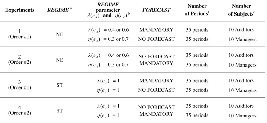
complexity of the experimental environment (Bloomfield and Wilks 2000; Libby et al. 2002). Each experiment consists of 35 periods of treatment NO_FORECAST and 35 periods of treatment MANDATORY_FORECAST. To minimize the carryover effect, two FORECAST orders are manipulated for each REGIME level: NO_MANDATORY (labeled “Order #1”) and Mandatory_NO (labeled “Order #2”). Each period simulates the one-period game between auditor and manager specified in section 3.1. Table 3 summaries the experimental design.

[Insert Table 3 here]

A notional currency called Experimental Dollars (EDs) is used in the experiments. In each experiment, all communications and interactions between players are handled by a system of networked personal computers. In the formal four experiments, the subject pool consists of 80 senior Business School students, with ten auditor-subjects and ten manager-subjects randomly assigned to each experiment. Students participate in two sessions. At the one-hour training session, subjects receive written instructions that are read aloud by the experimenter.5 _{Immediately following the} training session is the two-hour experiment session. All subjects draw to determine the role they will play in the experiment and the experimental periods then commence. At the beginning of each period, each manager-subject is endowed with 12,000 EDs and each auditor-subject is endowed with 10,000 EDs. Each subject plays the same role throughout all 70 periods. Upon completion of all experimental periods (the steps for each experimental period are described below), subjects are asked to complete a post-experimental questionnaire, paid their earnings privately in cash, and dismissed. The average cash earnings paid to the students is US$33.97 (ranging from US$27.91 to US$37.51). All four experiments take about three hours to finish.

The steps for each experimental period are described below:

5_{After clarifying questions are answered, a quiz (consists of ten true-false questions) is given to ensure that all subjects have} understood the instructions and how their decisions might affect their cash payments. All subjects are paid US $0.10 for each question they answer correctly (the average cash paid to the subjects is US$0.98, with the range being from US$0.87 to US$1). The experimental instructions and all related materials are available from the author upon request.

Step 1: At the beginning of each period, the computer randomly assigns each auditor to a manager.

Auditors are not informed of their assigned managers. This “manager-auditor” relation holds in that period only because my model does not consider auditor’s and manager’s reputation effect.

Step 2: At the beginning of each period, each manager-subject determines the earnings forecast to be

released by choosing either “Forecast High Earnings” or “Forecast Low Earnings” on the computer screen. This becomes the manager-subject’s private information.

Step 3: Each manager-subject is then provided with two investment alternatives: a low-cost investment low

I (with an effort cost of 1,000 EDs) and a high-cost investment I_high (with an effort cost of 2,500 EDs). All manager-subjects know that if Ilow (or Ihigh) is undertaken, there is a 0.80

probability of receiving an L earnings level (or an H earnings level) and a 0.20 probability of receiving an H earnings level (or an L earnings level). Manager-subjects can only choose one investment to undertake.

Step 4: The manager-subject privately determines the investment to be undertaken by choosing either

“High Investment” or “Low Investment” on the computer screen. This becomes the manager-subject’s private information.

Step 5: The realized earnings is determined by the computer and is shown on each manager-subject’s

screen. The manager-subject determines the earnings report by choosing either “High Earnings” or “Low Earnings” on the computer screen.

Step 6: The manager-subject pays a flat audit fee 3,000 EDs to hire an auditor-subject to credibly

verify the outcome of the investment.

Step 7: Each auditor-subject privately determines the effort level to be exerted by choosing either

“High Effort Level” (with an effort cost of 2,300 EDs) or “Low Effort Level” (with an effort cost of 1,700 EDs) on the computer screen. Each auditor-subject knows that if the realized earnings is H, he will always obtain a “High” audit signal SH with probability one. If the

realized earnings is L, the auditor-subjects will obtain a “Low” signal SL with probability 0.7 if he exerts high

A

e but will obtain the correct signal with probability 0.3 if he only exerts low A

e .

Step 8: Based on the auditor-subject’s effort choice and the realized earnings, the computer determines

the audit signal according to the probability distribution specified in Step 7.

Step 9: Upon observing the audit signal, the auditor-subject privately determines the audit report by

choosing either “High Earnings Report” or “Low Earnings Report” on the computer screen based on the reporting rules and the corresponding legal liabilities specified in section 3.1.

Step 10: Each player’s payoff is determined and the experimental period terminates.

4. EXPERIMENTAL RESULTS

Several points related to the experimental results are worth noting. First, the data set of 80 observations comprises 20 independent replications of each of the four experiments. One observation represents the average behavior of the overall 35 experimental periods played by the same auditor- or manager-subject under either the MANDATORY or NO_MANDATORY treatment. Second, in analyzing the data, the AFind rate is measured by the ratio of the number of periods each auditor-subject

issues an Hˆ report when he observes an SL signal divided by the total number of periods the subject obtains an SL signal, no matter whether there is a lawsuit against the auditor due to a bad state of

economy. This measurement is more relevant to the policy makers because it is the violation of

independence per se that is of particular interests for regulation purposes. Similarly, the AFtec rate is

measured by the ratio of the number of periods each auditor-subject obtains an SH signal when the true investment outcome is L divided by the total number of periods the subject obtains an SH signal, no matter whether there is a lawsuit against the auditor. Finally, to assist the discussions of the experimental results, I use FC_NE, NO_NE, FC_ST, and NO_ST to denote the four combinations of forecast mechanisms and legal regimes.

4.1 Players’ Behavior under Different Legal Regimes (tests of Hypotheses H1, H2, H3, and H4): Hypotheses H1 and H2 predict two competing equilibrium strategies for the manager and auditor under the FC_NE and FC_ST systems, respectively. Panels A-1 and A-2 indicate that hypotheses H1-(a) and H2-(a) seem to be the prevailing equilibrium in the experiments.

[Insert Table 4 here]

In contrast, hypotheses H3 predicts two competing equilibrium strategies for the manager and auditor under the NO_NE system and hypothesis H4 predict that NO_ST systems will (a) induce the manager to undertake I_high and always report truthfully when the investment outcome is L, and (b) motivate the auditor to exert low

A

e and remain independent. Panels B-1 and B-2 indicate that hypotheses H3-(a) and H4 are the prevailing equilibria in the experiments.

4.2 Players’ Reputation and Ethical Concerns (tests of Hypotheses H5 and H6):

In hypothesis H5, we posit that manager-subjects’ reputation concerns about the correspondence between their earnings forecasts and investment decision may explain their deviation from model’s point prediction. To test this hypothesis, we follow Stevens (2002) and capture each manager-subject’s reputation concerns (denoted by REPUTATION) through his / her response to the following statement in the post-experimental questionnaire, which ranges from 1 (strongly disagree) to 7 (strongly agree):

The correspondence between my forecast and Player A’s verification report is important to my investment decision.

Part (1) in Panel A of Table 5 displays summary statistics of the FH_IH rate (measured by the average frequency of each manager-subject’s undertaking Ihigh, given he / she forecasts FChigh, across two forecast mechanisms) and REPUTATION. Part (2) shows that the Pearson and nonparametric Spearman correlation coefficients between FH_IH and REPUTATION are 0.4581 and 0.4167, respectively, which are both significant at the 1% level. To test H5 in a more complete and precise way, we employ the following multivariate model:

FH_IH = a + b1(REPUTATION) + b2(LOSS) + b3(REGIME)+ b4(ORDER) + ε,

where FH_IH = The average f(Ihigh|FChigh) across two forecast mechanisms;

REPUTATION = Subject’s reputation concerns about the correspondence between

earnings forecast and investment decision, ranging from 1 - 7;

LOSS = The average amount of low high

C paid by each manager-subject;

REGIME = 0 for the NE regime and 1 for the ST regime;

ORDER = 0 if the FORECATS order is MANDATORY_NO and 1 if the FORECAST

order is NO_MANDATORY; ε = the residual term.

Variable LOSS is included in the regression model to control for the possibility that manager-subjects undertake Ihigh more often than the model prediction simply because they want to avoid the large loss low

high

C . Hypothesis H5 implies b1 > 0. Part (3) in Panel A of Table 5 indicates that

the bootstrap regression coefficient ˆb₁= 0.04606 is significantly greater than zero at the traditional significance levels (one-tailed). 6 Therefore, hypothesis H5 is supported, suggesting that manager-subjects’ reputation concerns do play an important role to their investment decision.

[Insert Table 5 here]

In hypothesis H6 we posit that auditor-subjects’ ethical concerns about compromising their independence may explain this deviation from model’s point prediction. To test this hypothesis, we follow Stevens (2002) and capture each auditor-subject’s ethical concerns (denoted by ETHIC) through his / her response to the following statement in the post-experimental questionnaire, which ranges from 1 (strongly disagree) to 7 (strongly agree):

To have accepted the extra payment 4,500 EDs from Player M and issued a High Outcome Report when you observe an L signal would have been unethical.

Part (1) in Panel B of Table 5 displays summary statistics of the AFind rate (measured by the

6_{The bootstrap-estimated parameters are computed from resampling of the original data. To test the significance of the} variables of interest, confidence limits are calculated using the bias-corrected and accelerated (BCa) method and are given three values of the significance level for each behavioral hypothesis: 1%, 5%, and 10% for H5 (one-tailed test of b1 > 0) and 90%, 95%, and 99% for H6 (one-tailed test of c1 < 0, see discussions on the next page). To achieve acceptable accuracy of the confidence limits, all parameters are estimated with 30,000 replications.

average AFind rate across two forecast mechanisms for each subject) and ETHIC. Part (2) shows that

the Pearson and nonparametric Spearman correlation coefficients between AFind and ETHIC are

−0.4996 and −0.4415, respectively, which are both significant at the 5% and 10% levels, respectively. That is, the auditor-subjects’ ethical concerns are negatively related to their independence-compromising decision. To test H6 in a more complete and precise way, I employ the following multivariate model:

AFind = a + c1(ETHIC) + c2(LOSS) + c3(ORDER) + ε,

where AFind = The average AFind rate across two forecast mechanisms for each subject;

ETHIC = Subject’s ethical concerns about compromising independence, ranging from 1 - 7; LOSS = The average amount of damage loss paid by each subject for committing an AFind

across two forecast mechanisms;7

ORDER = 0 if the FORECATS order is MANDATORY_NO and 1 if the FORECAST

order is NO_MANDATORY; ε = the residual term.

Variable LOSS is included in the regression model to control for the possibility that auditor-subjects compromise independence less often than the model prediction simply because they want to avoid the large damage loss Dind. Hypothesis H6 implies c1 < 0. Part (3) in Panel A of Table 5

indicates that the bootstrap regression coefficient ˆb₁= −0.022143 is significantly less than zero at the 5% significance levels (one-tailed). Therefore, hypothesis H6 is supported, suggesting that auditor-subjects’ ethical concerns do play an important role to their independence behavior.

In summary, the bivariate correlations and multivariate bootstrap regression results provide consistent support for both behavioral hypotheses. In this regard, our study not only contributes to the literature in auditor’s legal liability and independence by showing the prominent effects of subjects’ reputation and ethical concerns on manager’s investment and auditor’s independence decisions, but

7_{I first calculate each auditor-subject’s “mean damage loss” by multiplying Dind (i.e., 11,200 EDs) by the ratio of the} number of periods each auditor-subject is held liable for an AFind divided by the total number of periods each auditor-subject compromises independence for each damage apportionment rule. Variable LOSS is then measured by the

also contributes to the experimental economics literature in auditing by investigating the predictive ability of an economic model using psychological factors such as reputation and ethics.

4.3 The Joint Effects of Forecast Mechanisms and Legal Regimes on Players’ Behavior:

Table 6 reports the repeated-measured ANOVA results on f(Ihigh|FChigh), f(RL|L, Ihigh, FChigh), eAhigh,

AFtec rate, and AFind rate. As presented in the table, the main effect of the between-subject variable REGIME is significant for all five dependent variables at the 1% significance level, suggesting that

legal regime alone plays an important role to auditor-subject’s effort and independence strategies and manager-subject’s reporting and investment decisions. In contrast, the within-subject variable

FORECAST is significant only for f(Ihigh|FChigh), f(RL|L, Ihigh, FChigh), high A

e and AFtec rate, suggesting

that forecast mechanisms may not have significant impacts on auditor-subject’s independence behavior.

[Insert Table 6 here]

5. SUMMARY AND CONCLUSIONS

This paper reports the results of four experiments designed to examine the effects of different combinations of the forecast mechanisms and legal regimes different legal systems on auditor’s effort choice, independence behavior, and manager’s investment and reporting decisions. The experimental economics methodology is used to test a series of economic and behavioral hypotheses derived from a one-period game model in which (a) the manager is mandated to make earnings forecast before undertaking an investment, (b) the manager provides the quasi-rents and side payment to induce the auditor to compromise his independence, and (c) the auditor may commit either a technical audit failure or an independence audit failure. The experimental results document several important findings. First, If the policy makers intend to enhance auditor independence and motivate more investments and truthful reporting, a system that consists of a mandatory forecast together with a ST regime is the most favorable one to achieve these goals. Second, the experimental results show the significant effects of

auditors’ ethical concerns and manager’s reputation concerns on their behavior. The existence of these effects suggests the necessity of considering human’s psychological factors in examining manager’s reporting, auditor’s legal liability, audit quality, and independence. Finally, the legal regime has a direct (indirect) effect on auditor’s (manager’s) effort and independence (investment and reporting) decisions while a mandatory forecast mechanism affects mainly on the manager’s investment and reporting decisions.

Several limitations and future research directions should be recognized. First, the experiments are designed and conducted based on a one-period model. Therefore, the effects of auditor’s and manager’s reputation cannot be examined. A direct extension of the study would be to extend the model and experiments into a multi-period setting. Second, the experiments have shown that manager’s investment decision and auditor’s effort and independence decision are affected by their reputation and ethical concerns. These results suggest that future game theoretical studies in auditor’s legal liability and independence should take these psychological factors into considerations in analyzing auditor’s and manager’s optimal strategies. Finally, prior studies in the area of psychology and behavioral accounting have shown that subjects’ tolerance for ambiguity (defined as the way subjects perceive and process information about ambiguous situations) may affect their decisions under uncertainty (Einhorn and Hogarth 1985; Ghosh and Ray 1992). Therefore, the experiments can be modified to investigate how tolerance for ambiguity may affect auditor’s and manager’s behavior.

FIGURE 1 Game Tree of the Modela

i I H H S ∧ H No ( )Ii ρ 1−ρ( )Ii L H R RH L R ( )eA q 1−q( )e_A L S ∧ L ∧ H δ _1−δ ind

AF AFind AFtec AFtec

( )eA 1−λ Yes _Noc b No b No H S δ 1−δ ∧ H δ 1−δ c No ( )eA λ i FC FH ST A No L S ∧ L No FH ST B Yes ( )eA η No ( )eA η 1− FH ST C FH ST D FH ST E FH ST F FH ST G FH ST H FH ST I FH ST J FL ST A FL ST B FL ST C FL ST D ESTFL FSTFL FL ST G FL ST H FL ST I FL ST J FH NE A FH NE B FH NE C FH NE D EFHNE FNEFH FH NE G FH NE H FH NE I FH NE J FL NE A FL NE B FL NE C FL NE D EFLNE FNEFL FL NE G FL NE H FL NE I FL NE J NF ST A NF ST B NF ST C NF ST D ENFST FSTNF NF ST G NF ST H NF ST I NF ST J NF NE A NF NE B NF NE C NF NE D NF NE E NF NE F NF NE G NF NE H NF NE I JNFNE

a_{The variables shown in this game tree are defined as follows: FC}

i denotes the manager’s financial forecast, where i ∈ {high, low}; Ii denotes the manager’s investment amount, where i ∈

{high, low}; H and L denote the high and low investment outcomes, respectively; ρ(Ii) denotes the probability that the outcome is H when the manager invests Ii amount; Rk denotes the

manager’s financial report, where k ∈ {H, L}; q(eA) denotes the audit quality when the auditor’s effort level is eA; SH and SL denote the audit signals that the investment outcome is H and L,

respectively;Hˆ and Lˆ denote the auditor’s high-outcome and low-outcome report, respectively; δ denotes the probability that the state of the economy is bad; AFind and AFtec denote

auditor’s independence and technical audit failure, respectively; λ(eA) denotes the probability that the auditor will be held liable by the court when an AFind occurs; η(eA) denotes the

probability that the auditor will be held liable by the court when an AFtec occurs; ST and NE denote the strict and negligence legal regimes, respectively. Letters A to J denote managers’ and

auditor’s possible payoffs under different game outcomes and legal systems (see Appendix for detailed descriptions).

b_{There is no audit failure under these two scenarios (no matter whether the state of economy is good or bad) because auditor’s report correctly informs the investors of the investment}

outcome and, thus, is not misleading.

c_{Even though an audit failure occurs under these two scenarios, the auditor is not held liable by the court because the state of economy is good and, therefore, the firm will not go bankrupt. In}

TABLE 1

Summary of Notations and Parameter Values

Variables Definitions Parameter Values*

(1) Investment Parameters:

i

I Investment project i ∈ {high, low}

ω Realized earnings from the investment ω∈ {H, L} )

(I_i

ρ Probability that the investment outcome is H ρ(Ihigh)=0.8, 2ρ(Ilow)=0.

(2) Manager’s Parameters:

FCi Manager’s earnings forecast i ∈ {high, low} i

M

e Manager’s effort level for undertaking investment Ii i ∈ {high, low} )

( i M

e

C Manager’s effort cost when his effort level is i M

e C(ehigh_M )= 2,500 EDs, C(elow_M )= 1,000 EDs

Rk Manager’s reported earnings amount k ∈ {H, L}

low high

C Cost if forecast is FChigh but reported earnings is RL 1,000 EDs

high high

B _{Benefit if forecast is} FChigh and reported earnings is RH 100 EDs

high low

C Cost if forecast is FClow but reported earnings is RH 200 EDs

low low

C Cost if forecast is FClow and reported earnings is RL 500 EDs

AC Adjusting cost if manager’s reported earnings is

different from auditor’s report 5,000 EDs

Mr Manager’s compensation when audit report is r MHˆ = 9,500 EDs, MLˆ= 4,800 EDs

SP Side payment paid by the manager to the auditor 4,500 EDs

SC Manager’s switching costs if auditor is dismissed 3,000 EDs

(3) Auditor’s Parameters:

F Audit fees 3,000 EDs

j A

e Auditor’s effort level j ∈ {high, low}

) ( j

A

e

C Auditor’s effort cost when his effort level is j A

e C(ehigh_A )= 2,300 EDs, C(elowA )= 1,700 EDs

ξ Audit signal obtained ξ ∈ {SH_{, S}L_}

) ( j

A

e

q Audit quality (probability of obtaining a correct signal) ( high)=0.7 A e q , ( low)=0.3 A e q

r Audit report type r∈{Hˆ,Lˆ}

ER Present value of all future quasi rents 5,500 EDs

(4) Legal Liability Parameters:

δ Probability that the state of economy is bad 0.6 )

( j

A e

λ Probability that the auditor will be held liable for AFind

NE regime: ( high) A e λ = 0.4, ( low) A e λ =0.6 ST regime: ( j) A e λ =1 ) ( j A e

η Probability that the auditor will be held liable for AFtec

NE regime: ( high) A e η = 0.3, ( low) A e η =0.7 ST regime: ( j) A e η =1

Dtec Total damage losses due to technical audit failures 7,500 EDs

TABLE 2

Comparisons of Equilibrium Predictions under Different Forecast and Legal Regime Combinationsa

Forecasts Mandatory Forecast No Forecast

Legal Regime Negligence Regime Strict Regime Negligence Regime Strict Regime

Equilibrium Equilibrium #1 (A) Equilibrium #2 (B) Equilibrium #1 (C) Equilibrium #2 (D) Equilibrium #1 (E) Equilibrium #2 (F) Equilibrium #1 (G) Manager’s forecast

strategy FChigh FChigh FChigh FClow NA NA NA

Manager’s

investment strategy Ihigh Ihigh Ihigh I low I low I low Ihigh

Manager’s reporting strategy when outcome is L Always report RH Always report RL Always report RL Always report RL Always report RH Always report RL Always report RL Auditor’s effort strategy ehighA low A e low A e low A e high A e low A e low A e Auditor’s reporting strategy when obtain SL Always report Hˆ Always report Lˆ Always report Lˆ Always report Lˆ Always report Hˆ Always report Lˆ Always report Lˆ Auditor’s AFind ratec 1.00 0.00 0.00 0.00 1.00 0.00 0.00 Auditor’s AFtec rated 0.0698 0.00 0.00 0.00 0.5455 0.00 0.00

a_{The equilibria shown in this table are obtained by solving the game using the parameter values specified in Table 1 (see Appendix 2 for details).} b_{Under the NE (ST) regime, there are two equilibria (a unique equilibrium) for each of the two damage apportionment rules.}

c_{The AF}

ind rate is measured by the conditional probability that the auditor issues an Hˆ report when the audit signal is SL, i.e., AFind ≡p(Hˆ |SL). d_{The AF}

tec rate is measured by the conditional probability that the manager reports RH and auditor obtains an audit signal SH when the true investment outcome is L, i.e., AFtec ≡p(L|SH,RH)≡ p(RH |L)(1−ρ(Ii))(1−q(eA))/[ρ(Ii)+ p(RH |L)(1−ρ(Ii))(1−q(eA))].

TABLE 3 Experimental Design Experiments REGIME a REGIME parameter ) (e_A λ and η(eA) b FORECAST Number of Periodsa Number of Subjectsc 1 (Order #1) NE ) (e_A λ = 0.4 or 0.6 ) (e_A η = 0.3 or 0.7 MANDATORY NO FORECAST 35 periods 35 periods 10 Auditors 10 Managers 2 (Order #2) NE ) (eA λ = 0.4 or 0.6 ) (e_A η = 0.3 or 0.7 NO FORECAST MANDATORY 35 periods 35 periods 10 Auditors 10 Managers 3 (Order #1) ST ) (e_A λ = 1 ) (e_A η = 1 MANDATORY NO FORECAST 35 periods 35 periods 10 Auditors 10 Managers 4 (Order #2) ST ) (e_A λ = 1 ) (e_A η = 1 NO FORECAST MANDATORY 35 periods 35 periods 10 Auditors 10 Managers a_{This study adopts a 2×2 factorial design with two between-subject variables: REGIME (manipulated at two levels: NE vs. ST) and FORECAST}

(manipulated at two levels: No vs. Mandatory). NE and ST denote negligence and strict legal regimes, respectively. Each experiment consists of 70 periods.

b_{Under the NE regime, the probabilities that the auditor will be held liable by the court when there is an AF}

ind and AFtec are λ(eA) and η(eA),

respectively. These two probabilities are both decreasing in auditor’s effort level. Conversely, under the ST regime the auditor will always be held liable if the investors sue the auditor, that is, these two probabilities are both equal to one. Therefore, in the experiments we manipulate λ(e_A)and

) (e_A

η at two levels (i.e., less than one vs. one) to reflect the fundamental difference between NE and ST regimes.

d_{The subject pool consists of 80 senior Business School students, with 10 auditor-subjects and 10 manager-subjects randomly assigned to each} experiment. All subjects draw to determine the role they will play in the experiments. At the beginning of each period, each manager-subject is endowed with 12,000 EDs and each auditor-subject is endowed with 10,000 EDs. Each subject plays the same role throughout all 70 periods.

TABLE 4

Players' Overall Behavior in Four Experimentsa

Panel A-1: Mandatory Forecast − Manager’s Behavior

f (FChigh )

Negligence Regime (NE) Strict Regime (ST) Experiment

Ordersa _Prediction Averageb

(A) Prediction Averageb (B) t tests between (A) and (B)c Order #1 (n = 10) 1.00 (0.1001)0.6686 1.00 (0.1373)0.7629 −1.7542* Order #2 (n = 10) 1.00 (0.0924)0.6943 1.00 (0.1391)0.7771 −1.5684 Overall (n = 20) 1.00 (0.0947)0.6814 1.00 (0.1348)0.7700 −2.4047** f (Ihigh | FChigh )

Negligence Regime (NE) Strict Regime (ST) Experiment

Ordersa _Prediction Averageb

(C) Prediction Average b (D) t tests between (C) and (D)c Order #1 (n = 10) 1.00 (0.1132)0.6977 0.00 or 1.00 (0.1323)0.7593 −1.1183 Order #2 (n = 10) 1.00 (0.1068)0.7141 0.00 or 1.00 (0.1199)0.7811 −1.3192 Overall (n = 20) 1.00 (0.1075)0.7059 0.00 or 1.00 (0.1234)0.7702 −1.7570* f (RL | L, Ihigh, FChigh )

Negligence Regime (NE) Strict Regime (ST) Experiment Ordersa Prediction Average b (E) Prediction Averageb (F) t tests between (E) and (F)c Order #1 (n = 10) 0.00 or 1.00 (0.1329)0.2417 1.00 (0.0351)0.7298 −11.2274*** Order #2 (n = 10) 0.00 or 1.00 (0.1531)0.2167 1.00 (0.0786)0.7214 −9.2721*** Overall (n = 20) 0.00 or 1.00 (0.1402)0.2292 1.00 (0.0594)0.7256 −14.5841***

TABLE 4

Players' Overall Behavior in Experiments (cont’d)

Panel A-2: Mandatory Forecast − Auditor’s Behavior

f (ehighA )

Negligence Regime (NE) Strict Regime (ST) Experiment

Ordersa _Prediction Averageb

(G) Prediction Averageb (H) t tests between (G) and (H)c Order #1 (n = 10) 1.00 (0.1342) 0.7286 0.00 (0.1335) 0.2114 8.6408*** Order #2 (n = 10) 1.00 (0.1205) 0.7057 0.00 (0.1216) 0.1971 9.3959*** Overall (n = 20) 1.00 (0.1247) 0.7171 0.00 (0.1244) 0.2043 13.0191*** f (AFind )

Negligence Regime (NE) Strict Regime (ST) Experiment

Ordersa _Prediction Averageb

(I) Prediction Averageb (J) t tests between (I) and (J)c Order #1 (n = 10) 1.00 (0.0545)0.6848 0.00 (0.2222)0.1667 7.1611*** Order #2 (n = 10) 1.00 (0.0906)0.6674 0.00 (0.2012)0.1817 6.9579*** Overall (n = 20) 1.00 (0.0733)0.6761 0.00 (0.2065)0.1742 10.2434*** f (AFtec )

Negligence Regime (NE) Strict Regime (ST) Experiment

Ordersa _Prediction Averageb

(K) Prediction Averageb (L) t tests between (K) and (L)c Order #1 (n = 10) 0.0698 or 0 (0.0444)0.1789 0.00 (0.0343) 0.0514 7.1944*** Order #2 (n = 10) 0.0698 or 0 (0.0513)0.1635 0.00 (0.0267) 0.0471 6.3572*** Overall (n = 20) 0.0698 or 0 (0.0474)0.1712 0.00 (0.0300) 0.0492 9.7277***

TABLE 4

Players' Overall Behavior in Experiments (cont’d)

Panel B-1: No Mandatory Forecast − Manager’s Behavior

f (Ihigh)

Negligence Regime (NE) Strict Regime (ST) Experiment

Ordersa _Prediction Averageb

(M) Prediction Averageb (N) t tests between (M) and (N)c Order #1 (n = 10) 0.00 (0.0508) 0.2143 1.00 (0.0731)0.7171 −17.8599*** Order #2 (n = 10) 0.00 (0.0540) 0.2371 1.00 (0.0852) 0.7057 −14.6882*** Overall (n = 20) 0.00 (0.0524) 0.2257 1.00 (0.0775) 0.7114 −23.2248*** f (RL | L, I )

Negligence Regime (NE)

f (RL | L, Ilow ) Strict Regime (ST) f (RL | L, Ihigh ) Experiment Ordersa Prediction Average b (O) Prediction Averageb (P) t tests between (O) and (P)c Order #1 (n = 10) 0.00 (0.0891)0.1460 1.00 (0.1101) 0.6817 −11.9548*** Order #2 (n = 10) 0.00 (0.1240)0.1677 1.00 (0.0908) 0.6800 −10.2991*** Overall (n = 20) 0.00 (0.1057)0.1569 1.00 (0.1009) 0.6808 −16.0355***