雷達車輛偵測及衝擊波技術應用於緊鄰路口號誌控制之研究

國

立

交

通

大

學

運 輸 科 技 與 管 理 學 系

博 士 論 文

雷達車輛偵測及衝擊波技術應用於緊鄰路

口號誌控制之研究

Radar Vehicle Detection and Shockwave

Techniques for Signal Control of Closely

Spaced Intersections

研究生： 曾明德

指導教授：卓訓榮 教授

雷達車輛偵測及衝擊波技術應用於緊鄰路口號誌控制之研究

Radar Vehicle Detection and Shockwave Techniques for Signal

Control of Closely Spaced Intersections

研 究 生：曾明德

指導教授：卓訓榮

國 立 交 通 大 學

運輸科技與管理學系

博 士 論 文

Submitted to Department of Transportation Technology and Management College of Management

National Chiao Tung University in Partial Fulfillment of the Requirements

for the Degree of Doctor of Philosophy

in

Transportation Technology and Management

July 2012

Hsinchu, Taiwan, Republic of China

雷達車輛偵測及衝擊波技術應用於緊鄰路口號誌控制

之研究

學生：曾明德

指導教授：卓訓榮

國立交通大學運輸科技與管理學系 博士班

摘 要

在尖峰時刻，市區或高速公路匝道附近，常常會有數個緊鄰路口

的交通擁塞問題，其中號誌控制不當也常是擁堵主因。而在作智慧型

的號誌控制中，車輛偵測器的車流偵測能力更是關鍵因子。因此本研

究從車輛偵測器開始研究，除了偵測傳統流量、速度之外，並偵測十

字路口衝擊波，並應用該衝擊波技術作緊鄰路口的號誌控制。

本研究首先針對雷達車輛偵測器，提出車種、車速的演算法。該

演算法以最佳辨識演算法為基礎，結合影像處理來學習，使用支持向

量機 (Support Vector Machine)來辨識車種、支持向量迴歸 (Support

Vector Regression)來估計車長及分辨車種。以市區道路蒐集到的真實

資料驗證，並比較 K-mean 及線性判別分析法 (Linear Discriminant

Analysis)後，証實支持向量機及支持向量迴歸可成功精確地辨識機車、

小車、大車及超大車等多種車長及推估其速度。

接著，本研究利用前述雷達偵測器的偵測結果，提出新的三個交

通參數:空車、有車及停車，並利用此三參數結合車流理論導出路口衝

擊波的偵測方法，而且也在模擬環境成功驗證其可行性及精確程度。

最後本研究，提出一個以傳統觸動控制為基礎的臨界路徑控制方

法，該方法以關鍵行車路徑來設計時相、依車流回堵情形動態調整路

徑時相最大綠燈時間並在萬一車流在綠燈停止不動時，切換時相以避

免路口容量損失。該方法中，並以衝擊波理論為基礎推估各臨界路徑

上需求綠燈時間，進而提出最佳化模式，求解各路徑最佳均衡綠燈時

間。另外，也在一個實際的緊鄰路口組成的群組路口，模擬運作情形，

比起傳統觸動模式有顯著改善。

Radar Vehicle Detection and Shockwave Techniques for

Signal Control of Closely Spaced Intersections

Student: Ming-Te Tseng

Advisors: Hsun-Jung Cho

Department of Transportation Technology and Management

National Chiao Tung University

ABSTRACT

A complementary metal-oxide semiconductor based radar with

sensitivity time control antenna is successfully implemented for advanced

traffic signal processing. The collected signals from the radar system are

processed with developed optimization algorithms for vehicle-type

classification and speed determination. In course of optimization, a video

recognition module is further adopted as a supervisor of support vector

machine and support vector regression. In the meanwhile, skew training

data set and numerous classification scenarios are used to test the classifiers.

Finally, the results are analyzed and compared.

Beside, this investigation provides two traffic flow detection methods

for oversaturated signalized intersection. The first method detects

intersection shockwaves by innovative traffic parameters involving stopped

duration, moving duration, and empty duration. The second method

provides upstream arrival rate and speed by shockwaves, signal timing, and

traffic flow model. This research has a contribution to the detection of

shockwaves and upstream traffic parameters under over-saturated condition

which traditional detectors cannot provide.

Finally, a novel actuated critical path control model for designing

signal timings on closely spaced intersections is presented in this study.

Shockwaves are utilized to dynamically adjust maximal green time for each

critical path with unstable traffic demands. Combined with path-based

progression, this methodology suggests a novel way to deal with closely

spaced intersections. A real network had been exemplified with

micro-simulation to illustrate the effectiveness of the proposed method. The

numerical example demonstrates a satisfying result compare to ordinary

full-actuated scheme.

誌 謝

首先，感謝指導老師卓訓榮教授，多年指導；尤其在其身兼交通

部科技顧問室主任，犧牲奉獻國家之餘，尚且撥空幫忙；師母周幼珍

老師的仁慈關愛，亦是深感於心。李義明老師給予的文章協助，也深

表謝意。也感激張新立老師、韓復華老師、莊晴光老師、彭松村老師

在論文口試時的指導；另外也感謝吳宗修老師及蘇昭明老師於實務應

用上的指導。

接著，感謝父親曾兩傳及母親侯秋蓮女士的含辛茹苦的栽培，太

太譚小珠在就學期間的支持，以及兩個小孩曾致淳、曾祐謙的可愛陪

伴!

最後，對於藍健綸博士的文章寫作協助，特別感謝。學弟黃恆、

怡穎、柏元、威廷、楷霖的協助也表謝意。

Table of Contents

2.1 Radar vehicle detection ... 6

2.2 Shockwave estimation ... 13

2.3 Signal control methods ... 17

III Research methodology ... 29

3.1 Radar vehicle detection algorithm ... 29

3.2 Three new traffic parameters ... 40

3.3 Shockwave detection ... 41

3.4 Upstream speed and flow detection ... 55

3.5 Signal control algorithm ... 57

IV Results and Discussion ... 67

4.1 Radar vehicle detection ... 67

4.2 Three new traffic parameters ... 75

4.3 Shockwave detection ... 78

4.5 Traffic signal control algorithm ... 84 V Conclusions ... 89 Reference ... 92

LIST OF FIGURES

Figure 2.1 Side-fired radar detector ... 6

Figure 2.2 Radar signal power over road surface ... 6

Figure 2.3 FMCW Radar concept ... 9

Figure 2.4 Doppler frequency in FMCW Radar ... 9

Figure 2.5 Time-frequency distribution of a moving vehicle In FMCW Radar ... 10

Figure 2.6 Shockwaves at an intersection ... 14

Figure 2.7 Shockwaves in flow-density curve ... 15

Figure 2.8 Shockwaves in time-distance diagram ... 15

Figure 2.9 Shockwaves and queue length detection in an intersection ... 16

Figure 2.10 Shockwaves in time-space domain for a signalized intersection ... 17

Figure 2.11 Actuated phase intervals ... 21

Figure 2.12 A maximum band along an arterial ... 26

Figure 3.1 (a) A picture of a vehicle passing through the detection area of a radar (b) The spectrogram of the vehicle in (a) ... 30

Figure 3.2 The flowchart of the vehicle detection algorithm ... 31

Figure 3.3 Video training and calibrating system ... 38

Figure 3.4 Moving, empty and stopped duration ... 41

Figure 3.5 (a) Ideal shockwaves (b) Ideal shockwaves and general shockwaves (c) Five shockwaves relations (d) Five shockwaves in time-space diagram ... 42

Figure 3.6 The relation between shockwaves ... 43

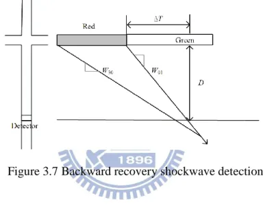
Figure 3.7 Backward recovery shockwave detection ... 45

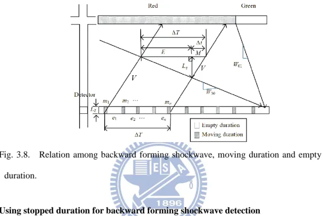
Figure 3.8 Relation among backward forming shockwave , moving and empty duration ... 48

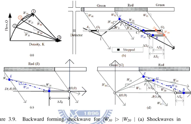
Figure 3.9 Backward forming shockwave for |W30 |> |W20 | ... 49

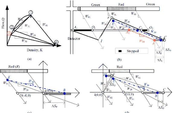
Figure 3.10 Backward forming shockwave for |W30 |< |W20 | ... 50

Figure 3.11 A vehicle‟s stopped duration is equal to red phase time ... 54

Figure 3.12 (a) The flowchart for five shockwaves detection. (b) The flowchart for backward forming shockwave detection ... 56

Figure 3.13 Four critical paths in three closely spaced intersections ... 59

Figure 3.14 (a) One-way progression in time-space diagram (b) Four-way Progression in path-intersection diagram ... 60

Figure 3.15 Full-actuated control with (a) gap out (b) max out when a vehicle stops on detection zone. ... 61

Figure 3.16 (a) Three traffic parameters: empty, moving and stopped durations (b) Enhanced actuated control with a “stopped out” condition. ... 62

Figure 3.17 Four critical paths in three closely spaced intersections ... 63

Figure 3.18 Flowchart of actuated critical path control algorithm ... 65

Figure 4.1 (a) Installation of radar sensor (b) The echo powers distribution for each lane of road ... 68

Figure 4.2 Block diagram of the proposed X-band FMCW sensor ... 69

Figure 4.3 Vehicle output lengths from SVR ... 74

Figure 4.4 Estimated vehicle speeds ... 74

Figure 4.5 Relationships between the three traffic parameters and VD distance from the stop bar ... 77

Figure 4.6 (a) Stopped, Moving and Empty durations in VD1 (b) Stopped, Moving and Empty durations in VD2 (c) △Stopped duration in VD1 and VD2 (d) Moving/(Moving+Empty) in VD1 and VD2 ... 78

Figure 4.7 The intersection of simulation ... 79

Figure 4.8 (a) The phase times of the intersection (b) The input flow of the link ... 79

Figure 4.9 (a) The stopped duration, moving duration and empty duration of detector 1 (b) The stopped duration, moving duration and empty duration of detector 2 ... 80

Figure 4.10 Relation between the stopped duration and red phase time ... 80

Figure 4.11 Results of the backward forming shockwave detection algorithm ... 81

Figure 4.12 Comparison of calculated / directly-measured shockwaves of the approach ... 82

Figure 4.13 The comparison of different arrival pattern and its

corresponding bias in shockwave estimation ... 83 Figure 4.14 The predicted traffic flow of state 3 ... 84 Figure 4.15 The predicted traffic speed of state 3 ... 84 Figure 4.16 Relation between the maximal green time and traffic

flow for proposed model. ... 87 Figure 4.17 Queue times of paths under (a) stable demand

(b) unstable demand. ... 87 Figure 4.18 Queue delay of paths under (a) stable demand

(b) unstable demand ... 87 Figure 4.19 Speed of paths under (a) stable demand

(b) unstable demand ... 88

LIST OF TABLES

Table 4.1 The specifications of radar sensor ... 67

Table 4.2 Set of vehicles used to test the classifiers ... 70

Table 4.3 The classification rate of classifiers ... 71

Table 4.4 Vehicles obtained from a field ... 71

Table 4.5 Leave-one-out recognition rate for different classifiers and categories. ... 72

Table 4.6 Leave-one-out error matrix for SVM( fm2)... 73

Table 4.7 Virtual loop length for each lane ... 74

Table 4.8 Summarized relationships between three traffic parameters and the environment. ... 76

Table 4.9 Experimental scenarios for model evaluation ... 85

I. Introduction

1.1 Background

Accurate methods of collecting traffic information are essential in an intelligent

transportation system (ITS). Traffic data has been gathered primarily via inductive loop

detectors, pneumatic road tubes, and temporary manual counts. However, traffic

detectors developed recently use video, sonic, ultrasonic, radar or infrared energy. These

detectors are non-intrusive and mounted either overhead or to the side of traffic lanes.

Considering the cost, radar and video sensors both have multi-lanes capability. A single

detector of either of these types can detect up to eight or ten lanes. However, poor

weather conditions, such as snow and heavy rain, can seriously impact video sensors. In

contrast, radar sensors still function effectively in poor weather. Therefore, radar sensors

are a good choice in ITS applications owing to their multi-lane coverage and resistance

to weather impacts.

Numerous classifiers have been developed and tested for data cluster or pattern

recognition, and these classifiers are categorized into two types: supervised and

unsupervised. In supervised learning, the aim is to learn a mapping from the input to an

output whose correct vehicle classes are provided by a supervisor. In unsupervised

learning, there is no such supervisor and we only have input of data. K-mean cluster is a

famous unsupervised classifier that has been used for numerous applications.

Furthermore, support vector machine (SVM) and linear discriminated analysis (LDA)

are two supervised classifiers. LDA was originally developed in 1936 by R.A. Fisher.

SVMs have been used for isolated handwritten digit recognition, object recognition,

speaker identification and face detection in images. To find the optimal classifier, this

a virtual loop concept that requires vehicle and virtual loop length to make an estimate.

Support vector regression (SVR) is used to predict vehicle length, while a video

calibrating system is used to measure virtual loop length. A skew training data set and

numerous classification scenarios are used to test the classifiers.

According to the Doppler Effect, the frequency of the radio wave will become

higher than the original frequency when the object approaches the radar device, and the

frequency of the radio wave will become lower than the original frequency when the

object moves away from the radar device. Therefore, the frequency variations of the

reflective signal is analyzed to acquire vehicle‟s speed; in other word, when a vehicle

moves at a high enough speed to generate the Doppler Effect, the reflective radio wave

from the vehicle will generate the Doppler shift. The Doppler frequency versus time

variations of the reflective radio wave is recorded and the relative speed of the vehicle

and the radar can be computed.

Real-time upstream traffic information is important because adaptive models must

have them to predict future traffic flow and compute the signal timing. Under

non-oversaturated situation, vehicle detectors can provide such real-time upstream

information. However, vehicle detectors are not capable to provide upstream flow

accurately under oversaturated traffic condition; vehicles often have a full stop at

detection zone and the detected flow is not “arrival” but “departure”. Hence, this

research utilizes another robust oversaturated traffic parameter, shockwave. The

shockwave detection methodology is also proposed to show its effectiveness.

To estimate shockwaves under oversaturated traffic situation, this research utilizes

innovative traffic parameters, including stopped duration, moving duration, and empty

Closely spaced intersections are characterized as having short link distance

between intersections; the physical spacing between the intersections is small. These

intersections often become traffic bottleneck during peak hours due to its physical

configuration. With inappropriate signal design and short links, traffic queues are likely

to spill-back and cause an inefficient signal operation. The jammed traffic is generally

derived from poor progression or unstable demands. Poor coordination of the signals

leads to queue spill-back from one intersection that can seriously disrupt operation of

the adjacent intersection. Furthermore, although several methods have been used to

mitigate the congestion of closely spaced intersection, they seldom focused on the

crooked traffics of the adjacent minor approaches. As the traffic demand on minor

approaches grows, progression on those approaches should also be introduced. Despite

the contribution of those researches, most of such models have not addressed such

progression issue. Traffics in closely spaced intersections are treated as paths in this

study. These paths would unfold hiding conflict points which would not easily be seen

while considering flows on different approaches only. These conflict points often cause

safety and efficiency issues, especially during oversaturated periods. Therefore,

progressions in these closely spaced intersections have a multi-path nature rather than

two-way progression on arterials.

1.2 Problem definition

The mixing of motorcycles and other traffic is hazardous in Asia. Currently, most

radar detection algorithms classify vehicles into three or five categories, but generally

exclude motorcycles from the classification system. How to detect motorcycles by radar

sensor should be focused. Beside, speed estimation is not accurate for single transceiver

Vehicle detectors are not capable to provide upstream flow accurately under

oversaturated traffic condition; vehicles often have a full stop at detection zone and the

detected flow is not “arrival” but “departure”. The shockwave is a robust detectable

parameter under oversaturated traffic condition and has been applied to traffic control

for a long time. An accurate estimation method for shockwave needs to be developed.

Closely spaced intersections often become traffic bottleneck during peak hours due

to its physical configuration. The jammed traffic is generally derived from poor

progression or unstable demands. Therefore, phasing sequence design and dynamic

green time adjustment need to be solved analytically.

1.3 Research objectives

The main objectives of this research effort can be summarized as follows:

To find a high recognition rate optimization algorithm for the vehicle-type

classification and speed determination of radar detector.

To provide two upstream flow estimation methods for oversaturated signalized

intersections; both methods are based on shockwaves of a signalized intersection. The

first method calculates shockwaves by combining the new traffic parameters and traffic

flow model. The second method makes use of the shockwaves derived from method one

and provides upstream flow estimation.

To find a signal control method to mitigate the oversaturated traffic condition in

closely spaced intersections.

1.4 Research contributions

This study illustrates a radar sensor classification scheme that classifies vehicles

successfully combine two supervised learning algorithms to do vehicle classification

and speed estimation: support vector machine and support vector regression.

The shockwave estimation method contributes 1) providing a general estimation

method for five shockwaves in an intersection, 2) the model formulation takes dynamic

signal timing into consideration, 3) the capability of predicting required green time to

discharge traffic queue, and 4) introducing an upstream flow estimation method that

capable to provide information beyond the detection zone of vehicle detectors.

The proposed signal control method which can: (1) improve signal operation by

path-based progression instead of two-way progression, (2) introduce a novel phase

change concept for full-actuated control to prevent capacity loss, and (3) modify

existing full-actuated control to suit the closely spaced intersections and to dynamically

adjust maximal green time according to unstable traffic demands.

1.5 Research layout

This dissertation is organized as follows. First, the introduction chapter gives an

overview of the background, problem definition, research objectives, contributions and

overview of this dissertation. Second, chapter 2 presents a literature review of related

researches in the relevant areas. The literature review chapter concerns about topics,

including: i) radar vehicle detection algorithms, ii) Shockwave detection and iii) signal

control methods.

Radar vehicle detection algorithm, shockwaves detection model and optimal signal

control algorithm for closely spaced intersections are proposed in chapter 3. In chapter 4,

numerical examples with real data for radar vehicle detector are discussed; shockwaves

and closely spaced intersections are simulated. The last chapter presents the conclusions

II Literature Review

This chapter provides literature reviews relevant to the formulation and solution algorithm of radar vehicle detection, shockwave estimation and closely spaced signal control problem. The following sections are organized as (i) radar detection algorithms, (ii) shockwave detection algorithms, (iii) signal control methods

2.1 Radar vehicle detection

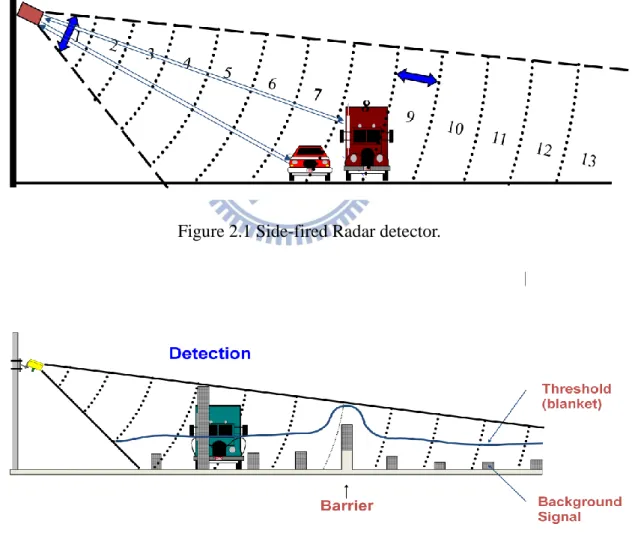
Figure 2.1 Side-fired Radar detector.

Microwave radar was developed for detecting objects. The word radar was derived

from the function that it performs: Radio Detection and Ranging. The term microwave

refers to the wavelength of the transmitted energy of 1GHz to 30 GHz. Microwave

sensors designed for traffic data collection are limited to intervals near 10.525 or 24.0

GHz. Sensors with 10.525GHz have lower range resolution , bigger size and lower cost

than sensors with 24Ghz.

Microwave sensors are generally mounted as side-fire configuration (as Figure

2.1). Side-fire mode is mounted on a roadside pole with its footprint aimed at right

angle to the traffic lanes. Side-fire mode can monitor up to 10 lanes for each sensor.

The sensor receives the reflected signals from all surfaces within its beam – pavement,

barriers, vehicles and trees. It maintains a background signal level from fixed objects in

each range slices. Vehicles are detected when their reflected signal exceeds the

background level of their range slice by a certain amount called threshold (see Figure

2.2).

The main types of microwave radar sensors are used in roadside are Frequency

Modulated Continuous Wave (FMCW) radar [1, 2] in which the transmitted frequency

is constantly changing with respect to time, as illustrated in Figure 2.3. The FMCW

radar operates as a presence detector and can detect motionless vehicles.

The carrier frequency increases linearly with time. The ramp slope is given byΔf/Δt.

The echo is received after the round trip time Tr = 2R/c where R is the distance to the

target. The echo is mixed with a portion of the transmitted signal to produce an output

beat frequency,

(2.1)

A moving vehicle will superimpose a Doppler frequency shift on the beat

frequency fd. One portion of the beat frequency will be increased and the other portion

will be decreased. For a target approaching the radar, the received signal frequency is

increased (shifted up in the diagram) decreasing the up-sweep beat frequency and

increasing the down-sweep beat frequency (see Figure 2.4)

fb(up) = fb - fd, (2.2)

fb(dn) = fb + fd.

If we look at the Doppler frequency when a vehicle passes through the radar

antenna beam, the Doppler shift of a reflected signal is proportional to the velocity of

the vehicle and to the angle at which the signal is reflected. This relationship is

described by the equation: For small angle Sinθ=θ, hence

(2.3)

Therefore, the Doppler shift changes linearly and pass through zero as the vehicle

pass through the sensor‟s field of view [3](As Figure 2.5). The slope of this linear

change is a function of the velocity of the target and the distance of the target‟s path

from the sensor. The Doppler shift of reflected angle is measured multiple times as the

vehicle passes through the field of view of side fire sensor. A linear fit is applied to the

Doppler shift measurements and results in a slope m. The slop m is converted to a speed

by

. (2.4) Another vehicle speed estimating method is to use the virtual loop concept [4, 5, 6],

Figure 2.3 FMCW Radar concept.

Radar Sensor θ d fd t V t2 t2 t1 t1 t3 t3 fd

Figure 2.5 Time-frequency distribution of a moving vehicle in FMCW Radar.

The speed of vehicle is calculated as

, (2.5) where L is the length of detection zone, Lv is the average effective length of

vehicles and Δt is the detector on time. The virtual loop speed can be a good result for

average speed. But it is not accurate in general.

Radar and inductive loop detectors have historically performed vehicle

classification by providing estimates of vehicle length based on vehicle speed ,v , and

the detector on time. The equation for vehicle length, Lv, is given by

H. Roe and G. S. Hobson (1992) [7] have described a forward-looking FMCW

Radar which can separate traffic into five classes. This single lane detector uses the

profile of vehicle to do vehicle classification. The profile is formed by the vehicle

height and length. The vehicle speed is calculated from Doppler effect. Park et al. (2003)

[8] have developed a FMCW side-looking vehicle detection radar. The velocity is

estimated by using the appearance duration of the reflected signal and the length of

detection zone and Doppler shift. The classification of a vehicle, as large, medium or

small size, is possible by processing received power and spectrum pattern

Numerous statistic learning methods have been developed and tested for data

cluster or pattern recognition, and these classifiers are categorized into two types:

supervised and unsupervised. In supervised learning, the aim is to learn a mapping from

the input to an output whose correct vehicle classes are provided by a supervisor. In

unsupervised learning, there is no such supervisor and we only have input of data.

K-mean cluster is a famous unsupervised classifier that has been used for numerous

applications. Furthermore, support vector machine (SVM)[9, 10] and linear

discriminated analysis (LDA) [11, 12] are two supervised classifiers. LDA was

originally developed in 1936 by R.A. Fisher [13]. SVMs have been used for isolated

handwritten digit recognition, object recognition, speaker identification and face

detection in images.

K-means is one of the best known data clustering methods. The goal of k-means is

to find k points of a dataset that best represent the dataset in a certain mathematical

sense. These k points are also known as cluster centers. After obtaining these cluster

centers, they can be used for data classification.

LDA is a supervisory classifier. LDA obtains a linear transformation ("discriminant

that provides more accurate discrimination than either predictor alone. A transformation

function is found that maximizes the ratio of between-class to within-class variance.

The transformation seeks to rotate the axes so as to maximize the differences between

the groups when the categories are project on the new axes. In the ideal case, a

projection can be found that completely separates the categories. However, in most

cases no transformation exists that provides full separation, so the objective is to obtain

the transformation that minimizes the overlap among the transformed distributions. The

LDA can be derived as a plug-in Bayes classifier. LDA projects the nine feature

dimension space considered in this study into a three dimension linear discriminant (LD)

space. The plug-in classifier finds the average group centers for each vehicle category

and saves it. When predicting a test sample vehicle, the classifier measures the

Mahalanobis distance between the group center and the LD project point of the vehicle

features. The plug-in classifier then estimates the posterior probability of each group

using Mahalanobis distance, the prior probability which is the group probability of

training set, and the covariance matrix. The testing vehicle belongs to the group with

the highest posterior.

SVM is also a supervisory classifier. SVMs attempt to identify a set of support

vectors, two support hyperplanes, and an optimal hyperplane for separating two groups.

SVM is a binary classifier. Two strategies can be developed to support multiple

classifications: one-against-one and one-against-rest. The one-against-rest strategy

constructs k SVMs to separate k groups. The m-th SVM separates the m-th group from

the others. For k groups, the one-against-one strategy constructs k(k-1)/2 SVMs to

2.2 Shockwave estimation

The theory of shockwaves had first developed by Lighthill and Whitham[14] .

Such shocks are generated at the discharge rates fall due to congestion or the

termination of a phase. The shockwave appears due to vehicle speed change, and this

configuration is very comprehensive to analyze traffic behaviors. As Figure 2.6 [15],

the trajectories of shockwaves were derived by assuming an average arrival rate at the

queue tail. It is noted that y1(0), y1(c) represent the initial and final queue length and the

line A1,C1,M1,D1,E1 the trajectory of the queue tail at which a shockwave is formed, l1

and l2 are the lost time during phase transitions and g1 is effective green time. By the

shockwave concepts at a signalized intersection, the required green time, queue length

and the end time of shockwave are listed as following equations.

The minimal green time for under-saturated approach is

1) (2.6)

The end time of shockwave A1,C1 is

) (2.7)

The final queue length for E1 is

t x B1 D 1 C M 3 2 L N c Y y (0) A y (c) 2 1 1 g1 l1 l2+g2 1 1 B1 , F1 1 E1 1

Figure 2.6 Shockwaves at an intersection [15].

A.D. May [16] have analysis the shockwave at signalized intersection as Figure 2.7.

A flow-density curve and approaching traffic flow states A, B, C and D are specified. A

distance-time diagram is shown in Figure 2.8 so that the slopes WAB, WBC, WAC and

WAD in two diagrams represent shockwave speeds. Then, the required green time to

discharge the traffic is

(2.9)

The maximal queue length is

(2.10)

Although some green time and queue length had been explored in the article, the

shockwave speeds are calculated by the flow and density difference between flow

A UA UC WAC C B D W B_C W AB WDB WDC W DA Density (veh/mile/lane) F lo w ( v eh /h r/ la n e) 0

Figure 2.7 Shockwave in flow-density curve[16].

D is ta n ce t0 t1 t2 B t3 A WAD A A Time A WAB B WCD D WAD T4 t5 t6 A A WDC D C _C WDB WAB WBC W AC

Figure 2.8 Shockwave in time-distance diagram[16].

Instead of counting arrival traffic flow in the current signal cycle, Xinkai et al.

(2009)[17] solve the problem of measuring intersection queue length by exploiting the

queue discharge process in the immediate past cycle. As Figure 2.9 , the authors find the

break points for A, B and C by detector occupancy time, and applying Lighthill–

Whitham–Richards (LWR) shockwave theory, the authors are able to identify the

Figure 2.9 Shockwaves and queue length detection in an intersection [17].

Shockwave analysis has long been applied to traffic flows [18, 19]. Shockwaves

are defined as boundaries in the time-space domain that indicate a discontinuity in

flow-density conditions [16], or the motion of a change in concentration and flow [20].

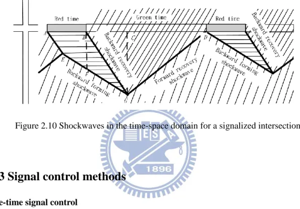
A typical time-space diagram at a signalized intersection is illustrated in Figure 2.10,

where the trajectories of individual vehicles are shown as thin black lines. Three types

of shockwaves are represented as thick black line segments:EG, a backward forming

shockwave; BG , a backward recovery shockwave; andGD, a forward recovery

shockwave [16]. Shockwave analysis can effectively analyze flow and queuing

problems [21, 22]; queue can be describe as BF and CGin Figure 2.10. Researchers

have applied shockwaves to compute delay (area AEGB in Figure 2.10) and green phase

time (BD in Figure 2.10) for traffic signals control [23, 24, 25]Numerous schemes have

also been proposed for plotting shockwaves and forecasting traffic system performance

[18, 21].

by traditional traffic parameters including volume, speed, and density [22, 26, 23, 25, 27,

28]. While others calculate shockwave by combining gap time, headway and speed [21],

or make use of high-resolution vehicle actuation data and signal information [29, 17,

30]. Skabardonis estimates upstream flow with flow, occupancy and phase timing while

traffic queue beyond vehicle detector[31] .

Figure 2.10 Shockwaves in the time-space domain for a signalized intersection.

2.3 Signal control methods

Pre-time signal control

The pre-timed control, which has fixed cycle lengths and preset phase times,

operates according to a predetermined time schedule. The pre-timed controllers are best

suited for locations with stable volumes and traffic patterns such as downtown areas.

Timing plans are usually selected on a time-of-day/ day-of-week basis. Although

pre-timed controllers have a degree of flexibility for daily traffic, they can cause

excessive delay when the traffic signal controller uses timing plans determined from

historical demands. The Webster method can be used to determine the optimum cycle

lengths for minimal delay.

the cycle length is obtained by the equation

(2.11)

where:

C = optimal cycle length (second); L = total lost time per cycle (second);

yi = the critical lane group volume (i th phase, vph) / saturation flow (vph);

n = number of phases.

The total lost time is the time not used by any phase for discharging vehicles. Total

lost time is given as

(2.12)

where:

li = lost time for phase i, which is usually 4 seconds; R = the total all-red time during the cycle.

The total effective green time, available per cycle, is given by

(2.13)

To obtain minimum delay, the total effective green time should be distributed

among the different phases in proportion to their y values to get the effective green time

for each phase,

(2.14)

The actual green time for each phase (not including yellow time) is obtained by

(2.15)

Actuated signal control

An actuated signal [33] operates with variable vehicular timing and phasing

intervals that depend on traffic volumes. The signals are actuated by vehicular detectors

placed in the roadways. The cycle lengths and green times of actuated control may vary

from cycle to cycle in response to demands. Actuated controllers include semi-actuated,

fully actuated, and density controllers.

In semi-actuated operation, the main street has a “green” indication at all times

until a vehicle or vehicles have arrived on one or both of the minor approaches. The

signal then provides a “green” phase for the side street that is retained until vehicles are

served, or until a preset maximum side-street green is reached. Non-actuated phases

may be coordinated with nearby signals on the same route, or they may function as an

isolated control. Non-actuated phases usually operate with fixed minimum green times

and may be extended by using green time that is not used by actuated phases with low

demand. That is, the green duration will be extended beyond the minimum green time

until a vehicle actuates the detector on the side street. At a semi-actuated controlled

intersection, detectors installed on the side street collect information for timing the

signal.

In fully actuated operations, all signal phases are controlled by detector actuations.

In general, each phase has a minimum green duration, but it also is shorter than the

maximum green time. A phase in the cycle may be skipped entirely if no demand exits

for that phase. The right of way does not return automatically to a specific phase under

the fully actuated mode unless recalled by a special setting in the controller. That is, the

controller shows green indication in the phase last served until conflicting demand

appears.

reduce the allowable gap according to several rules as vehicles show up or as time

progresses. The specifications allow gap reduction based only upon time waiting on the

red. This type of controller also has a variable initial interval, thus allows a variable

minimum green. Detectors are normally place farther back of the intersection stop line,

particularly on high-speed approaches to the intersection of major streets.

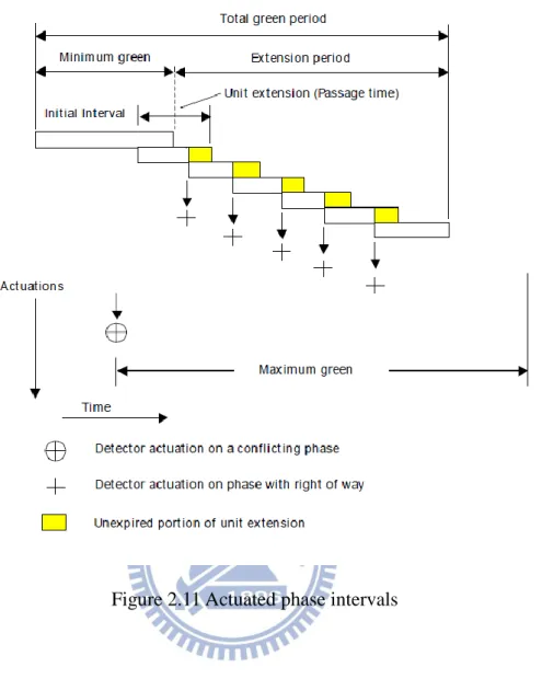
The timing characteristics of actuated signal operation are introduced here. In an

actuated phase, there are three timing parameters: the minimum green interval, the unit

extension, and the maximum green interval. These intervals are a function of the type

and configuration of the detectors installed at the intersection. These three intervals are

shown in Figure 2.11. This figure shows a case that the phase terminates before it

reaches the maximum green period because there is no vehicular actuation in the last

unit extension period.

The unit extension is time by which a green phase could be increased during the

extendable portion after an actuation on that phase. It depends on the average speed of

the approaching vehicles and the distance between the detectors and the stop line.

Initial interval is the first portion of the green phase that is adequate to allow

vehicles waiting between the stop line and the detector during the red phase to clear the

intersection. This time depends on the number of vehicles waiting, the average headway,

and the starting delay.

The minimum green interval is the shortest time that should be provide for a green

interval during any traffic phase. In basic design of actuated phase intervals, the

Figure 2.11 Actuated phase intervals

The maximum green interval is the limit that a phase can hold green in the

presence of conflicting demand. Normal range of maximum green is between 30 and 60

seconds depending on traffic volumes. Webster‟s model for pre-timed controllers can be

used to compute the maximum green interval. The computed green intervals are

multiplied by a factor ranging between 1.25 and 1.50 to obtain the maximum green.

Traffic-actuated controllers automatically determine cycle lengths and phase

durations based on detection of traffic on the various approaches. The cycle lengths and

green times are random variables, which depend on the real-time traffic demand.

Synchro software

Synchro [34] is a macroscopic and deterministic signal timing tool. Synchro has

the following features: it is able to simultaneously optimize lead-lag phase ordering in

addition to cycle lengths, phase lengths, and coordinated offsets, Percentile Delay

estimation method, data input and comprehensive output options, capability of

modeling RTOR, U-turns and six-legged intersections, capability of modeling

signalized and signalized intersections and roundabouts and it allows exporting its files

to CORSIM and HCS.

Synchro implements the HCM 2000 procedures for signalized intersections

capacity and delay calculation. Also, it possesses percentile delay calculation method

and intersection capacity utilization (ICU) 2003 methods. The basic premise of the

percentile delay method is that traffic arrivals follow a Poisson distribution. The

percentile delay method calculates vehicle delays for five different scenarios (i.e., 10th,

30th, 50th, 70th and 90th percentiles) and takes a volume weighted average of delays

predicted for each scenario. The ICU method sums the amount of time required to serve

all movements at saturation for a given cycle length. It is similar to taking sum of

critical volume to saturation flow ratios (v/s), yet allows minimum timing to be

considered. The ICU can tell how much reserve capacity is available or how much the

intersection is overcapacity.

Synchro does not use the Genetic Algorithm for optimization of signal timings.

The optimization objective function available is minimizing the percentile delay. It

optimizes the four signal timing parameters by evaluating a series of cycle lengths,

The best cycle length is found by calculating a performance index (PI).

The PI is calculated as follows.

(2.16) where

PI = Performance Index;

D = Percentile Signal Delay (s);

QP = Queue Penalty (vehicles affected);

ST = Vehicle Stops (vph);

D= ;

VD10 = 10th percentile Vehicle-Delay per

hour;

v10 = 10th percentile volume rate (vph).

TRANSYT 7F

TRAffic Network StudY Tool (TRANSYT) is one of the most widely used signal

timing programs. The original version of TRANSYT was developed by Dennis

Robertson at the Transportation and Road Research Laboratory in UK in 1967. Though

TRANSYT is most commonly used as an offline optimization tool, it may also be used

in an online fashion to compute signal settings every few minutes and download these

settings to the field. TRANSYT is a macroscopic, deterministic simulation and

optimization model. The model requires the link flows and link turning proportions as

inputs and assumes them to be constant for the entire simulation period. The program

optimizes splits and offsets given a set cycle length and carries out a series of iterations

module. TRANSYT-7F (Traffic Network Study Tool, version 7, Federal) [35] was

“Americanized” for the Federal Highway Administration (FHWA) in 1981 by the University of Florida Transportation Research Center. TRANSYT-7F Release 10.1

introduced in January 2004 included the ability to optimize cycle length, phase

sequence, green splits and offsets using a genetic algorithm (GA) and a traditional

hill-climb technique. Recent versions of TRANSYT-7F introduced the CORSIM

simulator in its optimization of cycle length, green splits and offset only. The

direct-CORSIM optimization in T7F consists of the CORSIM simulator and the GA

optimizer. It uses the CORSIM input file (*.trf) as an input so that T7F can directly

import all information related to the network and signal timing plan from the CORSIM

input file.

TRANSYT-7f includes detailed simulation of platoon dispersion, queue spillback,

queue spillover, traffic-actuated control, and the flexibility to perform lane-by-lane

analysis. Beside link wise simulation, TRANSYT-7F provides stepwise simulation

which updates all links one time step at a time. With stepwise simulation,

TRANSYT-7F can explicitly model queue spillback condition. TRANSYT-7F provides

left-hand drive right-hand drive option and it can only simulate two-way stop-controlled

(TWSC) intersections. HCS files can be loaded directly into T7F and timing plans can

be exported from T7F to HCS. Many traffic principles embedded in TRANSYT-7F such

as arrival type, delay calculation, level of service, capacity calculation and saturated

flow calculation are based on HCM 2000 procedures. TRANSYT-7F includes measures

of effectiveness (Throughput) for use in optimization of congested networks.

TRANSYT-7F has twelve distinct criteria. These criteria include functions designed to

The performance index (PI) may be defined as follow: PI= (2.17) MAXBAND

In 1966, John D. C. Little and his research colleagues at MIT defined the new state

of the art, called MAXBAND[36, 37, 38], ending with a set of algorithms to

synchronize fixed-timed traffic lights for streets with two-way traffic. It is one of the

representatives of the Fixed-Time Coordinated Control Strategies. By their nature,

fixed-time strategies are only applicable to under-saturated traffic conditions.

MXBAND considers a two-way arterial with n signals from S1 to Sn (intersections)

and specifies the corresponding offsets in order to maximize the number of vehicles

traveling at given range of speed without stopping at any signal (green wave).

MAXBAND considers splits as given (in accordance with the secondary street

demands); hence the problem consists in placing the known red durations of the

arterial‟s signals to maximize the inbound and outbound bandwidths In_B and Out_B, respectively (See Figure 2.12). In order to make MAXBAND work for a network of

arterials, Little (1966) extended the basic MAXBAND method by incorporation of

some cycle constraints. MAXBAND used into several networks into North America and

Figure 2.12 A maximum band along an arterial [36].

The underlying optimization model in MAXBAND is a Mixed Integer Linear

Programming (MILP) model. MAXBAND include its freedom to provide a range for

the cycle time and speed and it can operate a traffic signal effectively through the

interlocking control of neighboring intersections. Its disadvantages are the lack of

incorporated bus flows, limited field tests and because it is based on off-line analysis, it

is impossible for it to cope actively with irregularities in the traffic environment.

MAXBAND optimizes the signal by maximizing arterial progression bandwidth.

The output of the program includes cycle time, offsets, speeds and order of left turn

phases to maximize the weighted combination of bandwidths. The program can

automatically choose cycle time from a given range, allow the design speed to vary

within given tolerances, select the best lead or lag pattern for left turn phases from a

specified set, allow a queue clearance time for secondary flow accumulated during red,

network in the form of a three artery triangular loop.

The limitation of Maximization existing bandwidth is that the progression bands do

not correspond to the actual traffic flows on the arterial links. Therefore, bandwidth

maximization will not always lead to optimal system performance in terms of stops,

delay, and fuel consumption.

Near researches

The jammed traffic of closely spaced intersections is generally derived from poor

progression, unstable demands and inefficient signal operation. Poor regression of the

signals leads to queue spill-back from one intersection to upstream intersections. To

solve the aforementioned problems, researches focused on oversaturated demand,

closely spaced intersections, and traffic flow theories should be considered together.

Abu-Lebdeh and Benekohal [23] had developed a traffic control method and queue

management procedures for oversaturated arterials. Chang and Sun [39] had optimized

an oversaturated network by utilizing a bang-bang like model for the oversaturated

intersections and TRANSYT-7F for the undersaturated intersections. Michalopoulos and

Stephanopoulos brought the concept of shockwave theory to traffic signal control [29].

Tian, Urbanik and Gibby [40] had an application of diamond interchange control

strategies on a site of six closely spaced intersections. Messer [41] had studied the

traffic operations at oversaturated, closely spaced signalized intersection by NETSIM

simulations. Liu and Chang [42] had an arterial signal optimization model to do with

queue spill-back and lane blockage. Existing researches usually paid attention to

through traffics of the arterial; however, they seldom focused on the crooked traffics of

the adjacent minor approaches. As the traffic demand on minor approaches grows,

progression on those approaches should also be introduced. Despite the contribution of

Existing full-actuated signal scheme can only be applied to arterials; not much it

can do while facing a path-based progression situation. Zheng and Chu [43] and

Skabardonis [31] suggest methods to dynamically adjust maximal green for

full-actuated control under oversaturated traffic. With adjustable maximal green,

full-actuated control scheme have the potential to adaptive to oversaturated demands.

However, full-actuated schemes are focused on approach or arterial; they never focused

on path-based progression. Therefore, they should be modified to suit the specific

III. Research methodology

In this chapter, some essential concepts of the critical path signal control of closely

spaced intersections are discussed. Begin with the introduction to Radar vehicle

detection algorithm, the brief introduction to three new traffic parameters is addressed

in section 3.2. Section 3.3 shows the shockwave detection at intersection. The

estimation for upstream flow and speed by shockwave concept is illustrated in section

3.4. A critical path signal control algorithm is introduced, in section 3.5.

3.1 Radar vehicle detection algorithm

The radar cross section (RCS) of a vehicle is the key information used in vehicle

classification and speed estimation. Figure 3.1 shows a sample RCS signal of a car

received from the installation of Figure 3.1(a). The closed area indicated by a dashed

line is the detection area of the radar detector. The profile of a vehicle signal resembles

a mountain, and different vehicles create different shaped mountains. The vehicle

classifier extracts features from the profiles and classifies vehicles accordingly.

The speed estimator also identifies features from the profiles and calculates the

vehicle speed. Vehicle RCS is influenced by radar height and angle, radar distance from

the first lane, vehicle speed, vehicle shape and vehicle distance to radar. Most of these

factors are only fixed on the completion of radar sensor installation. Restated, the

vehicle profiles were completely changed when the environmental installation was

adjusted. This is a constraint for the supervised classifier, which needs to be retrained

for each new environmental installation. Generally, traffic managers hope that sensor

setup minimally impacts traffic condition. It means that the sensor setup time must be

If a training classifier is provided, the learning data is gathered during setup. Short setup

time results in a skewed distribution of vehicle types. The number of cars may be large

while the number of trucks is few. This forms the second constraint: short training time

and skewed training data.

Figure 3.1 (a) A picture of a vehicle passing through the detection area of a radar

detector. (b) The spectrogram of the vehicle shown in Figure (a).

Figure 3.2 presents a flowchart of an algorithm for these two constraints. The

algorithm includes four phases, namely signal processing, calibration, learning and

„classification and speed estimation‟. The rectangles which are enclosed by a dashed line comprise four major phases: signal processing, calibration, learning and

„classification and speed estimation‟. After retrieving the radar signal, a high pass filter is applied to filter background clutter signals. Fast Fourier transformation is to get the

range profiles of vehicles on lanes. Then, a constant false alarm rate (CFAR) thresholds

are used to detect the presence of vehicles. If the calibrating work is needed, the video

calibrating system will be used to calibrate the virtual loop lengths. When the

calibrating job is finished, the vehicle profiles will be complemented by the range of

step is to extract nine features from the complemented vehicle profile. While the

training job has never been done before, these features will be saved in vehicle training

database. The category and length of vehicle, which is the output of video recognition

system, will be saved into training database, too. If the number of vehicles is bigger

than a threshold, SVM and SVR will finish the learning step. When the learning job is

done, SVM will use vehicle features to classify vehicle‟s category. Finally, SVR will

predict the length of vehicle and output the vehicle speed. The details of the algorithm

will be presented in following subsections. The pseudocode of algorithm is shown as

following.

Figure 3.2 The flowchart of the vehicle detection algorithm. Online training ?

Retrieve the signal High pass filter Fast Fourier transfer

CFAR detection

Feature Extraction

SVM Traning SVM classification

SVR regressing SVR predicting Vehicle training Database :

Category, Length, Features Video traning system

Vehicle > n ? Output vehicle

category

Output vehicle

speed Speed estimation

Stop training Range complement

Find vehicle profile

Virtual loop length Video calibrating system Online calibrating ? Stop calibrating Each lane OK ? no yes yes no no yes yes no Begin Calibration Signal processing Learning Classification

Void Vehicle_classifier_and_speed_estimation_algorithm() begin while true Signal_processing(); if need calibrating Calibrating(); endif if vehicle<n Feature_extracting(); endif if need training Learning() endif if training done Vehicle_classification_and_speed_estimation(); endif endwhile End void Signal_processing() begin

retrieve signal from system;

apply high pass filter; do fast Fourier transform;

find vehicle profile; end

void Calibrating() begin

for each lane of street

check vehicle in/out by vehicle profile and clutter-map CFAR threshold if vehicle-in

capture vehicle-in image from video endif

if vehicle-out

capture vehicle-out image from video

compute virtual loop length by vehicle-in-out images classify vehicle category by images

compute vehicle length by images compute speed

save above results into training database endif endfor end void Feature_extrating() begin if vehicle-out

compute square energy

compute sum,maximal, mean and mean square error of vehicle magnitude profile

compute vibration of vehicle profile compute square vibration

save all features into database endif

end

void Learning() begin

retrieve vehicle features from database

retrieve vehicle length, speed, type, and loop length from database do SVM training do SVR regression end void vehicle_classification_and_speed_estimation() begin do vehicle classification by SVM do vehicle length prediction by SVR estimate vehicle speed

Signal processing

Most of the signal processing is performed during this phase. A discrete signal

frame xt[n] is retrieved from the time domain during a pulse interval t. Each discrete

signal frame has 128 points (n=1..128), and there are a total of 1500 signal frames per

second (pulse repeating frequency =1500). Since noise and background clutter disturb

normal vehicle echo signals, a simple high pass filter H(z)=1-z-1 is used to cancel the

background clutter. The filtered signal yt[n] is shown in Eq. (3.1).

yt[n]=xt[n]-xt-1[n] (3.1)

Furthermore, the high pass filter can also emphasizethe moving of vehicles. Since

a high magnitude of some frequencies means that some vehicles present on some lanes,

fast Fourier transform (FFT) is performed on yt[n] to get the frequency domain data

Yt[n]. That is to say, when a vehicle is presented at distance 3*n meters at time t ,

|Yt[n]| is great than some threshold. To avoid false alarms of vehicle presence, the

clutter-map constant false alarm rate (CFAR) [44] technique is adopted. The basic

characteristic of clutter-map CFAR is that the false alarm probability remains

approximately constant in clutter by a dynamic threshold. Vehicles with an echo power

exceeding the threshold thus can still be detected. Eq. (3.2) shows the clutter-map

CFAR threshold for the range n during pulse t.

) ] [ ) 1 ( ] [ ( ] [n Y 1n Y 2n Tt  t    t (3.2) where α=2 and γ=0.9.

The final step in signal processing is to collect the vehicle profile Vt[m] presented

at m-th range bin Yt [m] during the time interval in which vehicle is presented on

detection area. All classification methods are based on the vehicle profile from which

features are extracted. Eq. (3.3) defines the profile of the vehicle signal. Each

magnitude of m-th range bin |Yt [m]| is multiplied by power k of range frequency fm to

compensate for the decay of received power.

Vt[m]= |Yt[m]|×fmk (3.3) (

where T1<t<T2 and T1 and T2 are the first and last detection times of a vehicle

which passes through the radar detection area.

Feature Extraction

Nine features need to be extracted from the vehicle profile, most of which are

based on the physical characteristics of the vehicle. First, the energy of the vehicle

profile is shown in Eq. (3.4). A large vehicle implies large RCS, which in turn means

high energy. Square energy is used to emphasize this characteristic. Other features are

obtained from the statistical parameters associated with the vehicle magnitude profile.

These features include the maximal, mean and mean square error for elements of Vt[m].



Another physical phenomenon of vehicles is the vibration of the vehicle profile.

Small vehicles have low vibration while large vehicles have high vibration. Eq. (3.5)

calculates vehicle vibration. To increase the weighting of these characteristics, the

and the energy is the same concept as doing mathematical integration. These features

of each vehicle profile form a point in the feature space.

| ) ( ) ( 1 2 1 m V -m |V Vibration t T T t t  



Learning and Classification

This section aims to identify a classifier for effectively classifying vehicles into

one of four categories: motorcycles, small, medium and large.

First, this study tries the K-means clustering (denoted as K-means). Here K-means

is used as a method of partitional clustering in which the numbers of clusters and

random centers are specified before starting the clustering process. The number of

clusters is set to four. An objective function is then defined as the sum of the square

distances between a point in a feature space and the nearest cluster centers. The standard

K-means procedure is then followed to minimize the objective function iteratively by

finding a new set of cluster centers. These cluster centers can reduce the value of the

objective function at each iteration. Here the maximal iteration is set to 10.

The next classifier is LDA, which is a supervisory classifier. LDA measures the

Mahalanobis distance between the group center and the LD project point of nine vehicle

features. The LDA then estimates the posterior probability of each group using

Mahalanobis distance, the testing vehicle belongs to the group with the highest

posterior.

The last classifier is SVM, which is also a supervisory classifier. SVM is a binary

classifier. The one-against-one strategy is developed to support multiple classifications

For k groups, the one-against-one strategy constructs k(k-1)/2 SVMs to separate each

pair of groups. This study tests SVM using the one-against-one approach, in which six

Prediction is performed by voting, where each classifier makes a prediction and the

most frequently predicted class wins (“Max Wins”). In cases where two groups receive an identical number of votes, this study simply selects the one with the smallest index.

For supervisory classifiers LDA and SVM, the environmental installation problem

leads to retraining of the classifier for each installation of radar sensors. To resolve the

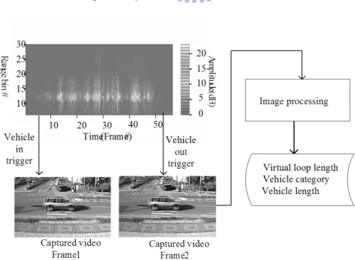
problem, this study proposes a learning method based on a video training system, as

shown in Figure 3.3. The system receives vehicle-in and vehicle-out triggers when a

vehicle is either inside or outside the detection area. After receiving the triggers, the

system captures two video frames. The image processing unit then outputs virtual loop

length, vehicle category and vehicle length. Using clutter-map CFAR, the radar system

can know the in and out time of a vehicle. When the radar system sends vehicle-in or

vehicle-out triggers to the video system, the video system immediately captures a video

frame. These two video frames can then be used to perform image processing to obtain

the vehicle type. The vehicle type and its features are saved in a training database which

can be used to train a supervisory classifier.

Calibration and speed estimation

In general, the radar speed detecting method is based on the Doppler principle.

When a radio wave bumps onto a tracked object, the radio wave is reflected, the

frequency and the amplitude of the reflective wave are influenced by the moving state

of the tracked object. If the tracked object is stable in its position, the frequency of the

reflective radio wave will not be changed and the Doppler effect will not be generated.

If the tracked object moves forward in the transmitted direction of the radio wave, the

frequency of the reflective radio wave will be increased; on the other hand, if the object

moves oppositely to the propagated direction of the radio wave, the frequency will be

decreased. As a result, the effects of the Doppler Shift are produced. However, the

Doppler effect is not obviously and stable for roadside fired Radar. It is almost zero

when vehicle pass through the detection zones. The RCS of vehicle is so complicated

such that equations 2.2-2.4 are not possible to be applied.

Hence, the vehicle speed is estimated using Eq. (3.6). The detection zone of each

lane forms a virtual loop. The key to correctly estimating the speed is to more precisely

calculate the three parameters of Eq. (3.6).

ΔT L L

Speed v z , (3.6) (

where L_v denotes the length of the vehicle, L_z represents the length of the

virtual loop and ΔT is the time of vehicle occupation.

It is easy to obtain the vehicle occupation time ΔT from clutter-map CFAR. The

length of the virtual loop L_zmust be carefully calibrated. The length of the virtual loop

is also an environmental installation problem. The length differs between environmental

installations. Theoretically, the virtual loop length can be obtained from radar equations,