整合模糊應用與圖形識別方法於台灣股價趨勢行為之發現

全文

(1)國立交通大學資訊管理研究所碩士論文. 整合模糊應用與圖形識別方法於台灣股價趨勢行為之發現. Using a Fuzzy-based Pattern Recognition Method to Discover Taiwan Stock Trend Behavior. 研究生：鄭啟斌指導教授：陳安斌. 博士. 中華民國九十三年六月.

(2) 整合模糊應用與圖形識別方法於台灣股價趨勢行為之發現 Using a Fuzzy-based Pattern Recognition Method to Discover Taiwan Stock Trend Behavior. 研究生：鄭啟斌. Student：Chi-Ping Cheng. 指導教授：陳安斌. Advisor：An-Ping Chen. 國立交通大學資訊管理研究所碩士論文 A Thesis Submitted to Institute of Information Management College of Management National Chiao Tung University in Partial Fulfillment of the Requirements for the Degree of Master of Business Administration in Information Management June 2004 Hsinchu, Taiwan, the Republic of China. 中華民國九十三年六月.

(3) 整合模糊應用與圖形識別方法於台灣股價趨勢行為之發現. 學生：鄭啟斌. 指導教授：陳安斌. 國立交通大學資訊管理學系﹙研究所﹚碩士班. 中文摘要台灣股市成立至今，累積了大量的時間性股市資料，在龐大資料庫中隱含著許多成功投資者的投資模式。股市交易是買賣雙方投資行為的結果，其受影響之因素有很多，例如政治、總體經濟、國際情勢、社會消息、成交量等因素均會影響投資行為。股價是一切因素的結果，因此，股價走勢圖可視為最具代表性之投資者行為模式。獨立成份分析(ICA)是一混合訊號分離的技術，可以由混合訊號中找出獨立元素或是潛在行為。而股價就如同混合訊號，是許多因素的綜合結果，因此本研究先利用獨立成份分析方法，發掘隱藏在股價之內的獨立成份，雖然無法了解每個成份本身代表何種因素，但是利用此方法，去除解釋股價能力較低之元素，使得股價的干擾減少，將有利於發現有意義有價值之股價走勢。圖形識別(Pattern Recognition)是近年來熱門的研究領域之一，其根據物體或是圖片的顏色、形狀等屬性、特徵來做辨認，通常是由已知的圖樣去找尋最相似的圖形，此方法已大量的應用在指紋比對、人臉辨識、語音辨識、簽名認證、數位浮水印等，本論文則企圖將圖形比對之方法應用於股市時間序列。本實驗由證券基金會(SFI)之資料庫收集自 1996 年 11 月 26 日至 2004 年 4 月 28 日台灣股市個股收盤股價日資料，利用圖形識別方法，針對當時個股股價的走勢，比對歷史股價中重覆出現的圖樣。本研究試圖提出一個新的比對方法，以減少比對的時間：先針對一段待測股價時間序列圖進行特徵抽取(Feature Extraction)，找出人類視覺上最重要的特徵點(Feature Points)，透過特徵點間的相關資訊進行比對工作，包括了圖形的角度以及相對長度。實驗結果找出了歷史中重覆出現的圖樣，也就是相似的走勢，證明了股價走勢有歷史重現的現象，據此可針對相似走勢的未來趨勢來作預測分析。實驗結果證明所提圖形比對方法之平均獲利較買進持有策略、最小平方法求得的趨勢線來的好，可作為投資人投資時的決策參考。關鍵字：特徵抽取、圖形識別、獨立成份分析、台灣股市. i.

(4) Using a Fuzzy-based Pattern Recognition Method to Discover Taiwan Stock Trend Behavior Student：Chi-Ping Cheng. Advisors：Dr. An-Ping Chen. Department﹙Institute﹚of Information Management National Chiao Tung University. Abstract There have been a large amount of stock data and valuable trading strategies stored in Taiwan stock market database. The stock price, impacted by various factors, is the result of buyer-seller investment decisions. The influencing elements consist of politics, economics, international statuses, and news information all around the world. Since the stock price is capable of reflecting the value-relevant information in the market, the stock patterns can be regarded as the behaviors of investors in the environment. Independent component analysis (ICA) is a technique for separating the mixture signals to find out the independent components or hidden factors. In this thesis, since stock price is a mixture signal, ICA can be used to extract the unknown independent components. In this way, by eliminating the component with lower effect is able to reduce the unnecessary noise and discover the significant trend patterns. Pattern recognition is one of the most popular research areas in recent years. The approach is used to identify the objects or images by their forms, outlines, colors or other attributes. The general purpose of pattern recognition is to find out the most similar patterns. The major applications of pattern recognition contain signature certification, digital watermarking, fingerprint, face and speech recognition, etc. In this research, pattern recognition is applied to finance time series mining for discovering the concealed knowledge in the stock market. In the thesis, the experimental data is collected from Securities & Futures Institute (SFI) on daily closing price of Taiwan Stock Exchange Weighted Stock Index (TAIEX). The simulation time period is from November 26, 1996 to April 28, 2004 for 1,942 trading days. The pattern recognition concept is used to match the current stock price trend with the ii.

(5) historical repeatedly appearing patterns. Accordingly, a new method is developed in the thesis to extract the features from the stock chart for discovering the most critical feature points. The matching procedure is processed through the corresponding information of the feature points, which is capable of reducing the experimental time. After the simulation, the historical repeatedly appearing patterns, namely the similar trend, will be discovered. The results show that the stock trends are continually occurring. Consequently, the future trend of matching patterns will be analyzed to offer investors the information for making strategies. Besides, the average profit of proposed model is higher than buy-and-hold strategy and the least square line.. Keyword: feature extraction, pattern recognition, independent component analysis, Taiwan stock market. iii.

(6) List of Contents 中文摘要 .....................................................................................................................................i Abstract .....................................................................................................................................ii List of Contents........................................................................................................................iv List of Table..............................................................................................................................vi List of Figure...........................................................................................................................vii Chapter 1 Introduction ............................................................................................................1 1.1 Motivation ....................................................................................................................1 1.2 Research Scope.............................................................................................................2 1.3 Objective.......................................................................................................................3 1.4 Thesis Organization ......................................................................................................3 Chapter 2 Literature Review...................................................................................................5 2.1 Overview of Stock Market ...........................................................................................5 2.1.1 Stock Market Volatility Factors .................................................................................5 2.1.2 Stock Market Analysis...............................................................................................5 2.2 Independent Component Analysis ................................................................................7 2.2.1 Blind source separation Problem...............................................................................7 2.2.2 Independent Component Analysis .............................................................................8 2.2.3 Preprocessing for Independent Component Analysis..............................................10 2.2.4 Application .............................................................................................................. 11 2.3 Pattern Recognition for Time Series........................................................................... 11 2.3.1 Indexing ...................................................................................................................12 2.3.2 Segmentation ...........................................................................................................15 2.3.3 Clustering and Classification...................................................................................16 2.4 Fuzzy Set Theory........................................................................................................17 Chapter 3 System Architecture .............................................................................................20 3.1 Reducing Noise in Stock Price ...................................................................................20 3.1.1 Objective..................................................................................................................20 3.1.2 Fast Independent Component Analysis ...................................................................22 3.2 Feature Extraction ......................................................................................................24 3.3 The Information about Adjacent Feature Points.........................................................27 3.3.1 The Angle of Adjacent Feature Points.....................................................................27 3.3.2 The Relative Length of Adjacent Feature Points.....................................................28 3.4 Similarity Matching....................................................................................................29 3.5 Trend Analysis ............................................................................................................31 Chapter 4 Simulation .............................................................................................................34 4.1 Data Description.........................................................................................................34 4.2 Model Parameters .......................................................................................................35 iv.

(7) 4.3 Independent Component Analysis ..............................................................................36 4.4 Data Normalization ....................................................................................................38 4.5 Pattern Matching and Analysis ...................................................................................39 4.6 Simulation Result .......................................................................................................43 Chapter 5 Analysis and Discussion .......................................................................................45 5.1 Comparison Models....................................................................................................45 5.1.1 Buy and Hold Strategy ............................................................................................45 5.1.2 Least Square Method ...............................................................................................46 5.2 Statistical Test.............................................................................................................47 5.3 Performance Discussion .............................................................................................50 Chapter 6 Conclusion and Future Work ..............................................................................52 6.1 Conclusion ..................................................................................................................52 6.2 Future Work ................................................................................................................52 References................................................................................................................................54. v.

(8) List of Table Table 1. Trading strategies........................................................................................................33 Table 2. Fourteen value-weighted stocks of the electronic industry in TAIEX ......................34 Table 3. The trading strategies..................................................................................................42 Table 4. The simulation result without reducing noise.............................................................43 Table 5. The simulation result with reducing noise..................................................................44 Table 6. An example of simulation trading of UMC ................................................................44 Table 7. The simulation of modified buy and hold strategic ....................................................45 Table 8. The trading strategies of least square method.............................................................47 Table 9. The simulation of least square method .......................................................................47 Table 10. The Average profit of three methods ........................................................................49. vi.

(9) List of Figure Figure 1. An example of similar trend patterns . ........................................................................2 Figure 2. The original signals and its mixtures ..........................................................................8 Figure 3. The basic procedure of ICA ........................................................................................9 Figure 4. Four basic classes membership function...................................................................18 Figure 5. The membership function of matching error ............................................................18 Figure 6. The procedure of approach........................................................................................21 Figure 7. Fixed-point algorithm for one unit............................................................................23 Figure 8. Pseudo code of the feature extraction on the time series ..........................................25 Figure 9. Time series of feature extraction ...............................................................................25 Figure 10. 8 cases when finding feature point in time series. ..................................................26 Figure 11. 2D pattern matching ................................................................................................27 Figure 12. The relative length of adjacent feature points .........................................................29 Figure 13. The first similarity measurement, angle..................................................................30 Figure 14. The second similarity measurement, relative length...............................................30 Figure 15. The membership function of similarity...................................................................31 Figure 16. The pseudo code of membership function ..............................................................32 Figure 17. The valid price fluctuation rate figure.....................................................................33 Figure 18. Different number of feature points..........................................................................36 Figure 19. The number of feature points and average error .....................................................36 Figure 20. The ordering eigenvalues ........................................................................................37 Figure 21. Eight dominate independent component.................................................................37 Figure 22. The reconstruction stock price.. ..............................................................................38 Figure 23. The stock price of UMC is for feature extraction. ..................................................40 Figure 24. The first membership function of similarity ...........................................................41 Figure 25. The second membership function of similarity.......................................................41 Figure 26. The concept of the profit rate ..................................................................................42 Figure 27. Right-tailed t test for mean difference ....................................................................48. vii.

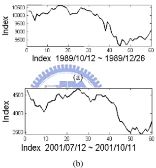
(10) Chapter 1 Introduction 1.1 Motivation Time series data mining and forecasting analysis are two important and popular issues in recent years. Time series data has been used extensively in many domains, including traffic and network flow, stock price, sales, and product quantity. Specifically, the research focuses on the stock market time series.. The stock exchange is influenced by many factors, such as politics, economics, international statuses, significant news, and so forth. The composite result from different factors will be reflected on the stock market. Since the stock price is the final consequence of various components, it is more meaningful and easily interpretable to illustrate the variation of stock price with the chart than listing numerical data. Hence, stock trend chart is one of the most useful and major tools for stock analysis.. Seelenfreund et al. (1968) used past price information to forecast the future price [7]. Lo et al. (2000) [5] proposed automatic approach stock pattern recognition. The patterns, head-and-shoulder and double-bottoms, are found for describing some phenomena in stock time series. Therefore, stock behavior and similar trend exist in the stock price. For example, in Figure 1, the two charts (a) and (b) respectively represent the stock trend on Taiwan Stock Exchange Weighted Stock Index (TAIEX) in different time durations. By human vision faculties, the two trend patterns look similar yet they were actually in two different time intervals, [1989/10/12, 1989/12/26] and [2001/7/17, 2001/10/11]. It is too subjective to tell the difference of the similar trend patterns in the stock database. Therefore, a new approach is developed and proposed in the thesis, and further discussion and analysis of the interesting. 1.

(11) phenomenon will be conducted.. Recently, behavioral finance has been getting more and more attention. When a person is making strategies, he is not always rational because of being affected by the mental elements. The daily stock price is closely related to the current, past, and future circumstances. Stock data mining, which obtains the knowledge through the relevant analysis, can help investors to make investment strategies.. (a). (b) Figure 1. An example of similar trend patterns (a) and (b).. 1.2 Research Scope The data source of the thesis comes from Securities & Futures Institute (SFI) on daily closing price of stock in Taiwan Stock Exchange Weighted Stock Index (TAIEX). The experimental time period is from 1996/11/26 to 2004/4/28, totally 1,942 days. The historical data before year 2002 is regarded as the past patterns, and the data from 2002/1/1 to 2004/4/28 is used to match and discover the similar patterns investment modeling. The factors, which influence the stock market, are not considered, including significant news, politics,. 2.

(12) economics, and international statuses. The basic assumption is that stock price reflects all factors.. 1.3 Objective. The documents and papers of stock analysis have been proposed and discussed for a long period of time. The most common and widely discussed categories of stock analysis are fundamental and technical analysis. In fundamental analysis, more professional financial knowledge is required due to the delayed releasing of financial statement. In technical analysis, the study of stock trend prediction is based on the historical price and volume. The rich experiences and subjective judgment of the investors are required for making profit.. In this thesis, an efficient pattern recognition method discovering significant pattern on the time series is proposed. The objective approaches are applied to the stock data to discover the significant investment patterns. Firstly, independent component analysis (ICA) is used to reduce the noise of the stock price. Secondly, feature extraction method is used to extract the most critical feature points in the stock time series. Thirdly, the matching approach among the feature points is done through their relevant information. The proposed approaches are useful and beneficial for investors to gain some knowledge from the stock market.. 1.4 Thesis Organization The rest content of this thesis is introduced as follows. In Chapter 2, the overview of stock market, independent component analysis, pattern recognition, and fuzzy set for time series are reviewed according to scholarly and literary methodologies. The proposed method implemented in this thesis consists of reducing noise by independent component, feature extraction, similarity matching, and trend analysis, will be elaborated in Chapter 3. The 3.

(13) simulation process and its results are illustrated in Chapter 4. In Chapter 5, the comparison of the experimental outcome on the proposed method, buy-and-hold strategy, and least square method will be presented. The performance of proposed method is discussed. Finally, some concluding remarks and future works are given in Chapter 6.. 4.

(14) Chapter 2 Literature Review 2.1 Overview of Stock Market Stock is a part of ownership of a company when people bought and held it. It is also one of the well-known investment tools. The stock factors and analysis methods will be discussed in the following section.. 2.1.1 Stock Market Volatility Factors. Stock price is influenced by various elements, three basic categories of which include stock market, industry, and corporation factors [8]. The determinants of stock market involve macroeconomics, international statuses, news [39], and domestic politics. Industry factors consist of industrial conditions, business cycles, and law measures. The dividends, operating performance, firm structure and restructuring are the corporate factors. To sum up, stock price is influenced by numerous unexpected factors. Some of them correspond to long-term trend, and some are short-term.. 2.1.2 Stock Market Analysis. In general, fundamental and technical analyses are used to examine the behavior of the stock market. Fundamental analysis focuses on company and macroeconomics factors. Company factors include including the economic growth rate, financial statement, operating performances, earning per share (EPS) [33] of the company and so on. Macroeconomics contains inflation, and unemployment, etc. The main shortcoming of fundamental analysis is that more professional financial domain knowledge is required and the delayed issue of financial statement. 5.

(15) Technical analysis concentrates on the historical movement of price and volume [5][30][31], which can be used to forecast the future trend. Brock et al. (1992) [40] use the simplest and the most popular technical trading rules, moving average (MA) and trading range break, to simulate on Dow Jones Industrial Average Index from 1897 to 1986. They obtain strong support in technical analysis. In addition, there are other important and commonly-used technical indictors that are computed by the price and volume, such as stochastic KD Line (KD), Moving Average Convergence-Divergence (MACD), Relative Strength Index (RSI), and so on. Lo et al. (2000) [5] mention that the main drawback of technique analysis is excessively subjective. Therefore, an objective approach of stock analysis is required.. Besides the fundamental and technical analysis, data mining techniques are also used to discover the trading rules in the stock market. Gavrilov et al. (2000) [25] show that normalization can refine the quality of the mining result. Scaling and translation will improve the simulation results. Furthermore, the piecewise normalization outperforms the normalization on the whole sequence. Piecewise normalization can reduce the local abnormality in two stocks. Since the raw data is not easily classified, reducing the dimension of experimental data seems to be quite important. Tsaih et al. (1998) [28] apply hybrid artificial intelligence to analyze S&P 500 Stock Index. The hybrid AI includes rule base system and back propagation neural network. To sum up, the fundamental and technical analyses have some shortcoming. Hence, an efficient and objective method should be proposed for stock analysis.. 6.

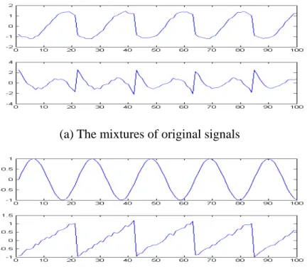
(16) 2.2 Independent Component Analysis. 2.2.1 Blind source separation Problem. In real world, noise is usually contained in the collected signals. Independent component analysis (ICA) [1][3][36] is a powerful technique for finding the hidden patterns from the mixture signal. For example, assume there are two persons talking in the same room at the same time. Two microphones are set in different corners of the room in order to record the speech signals, denoted as x1(t) and x2(t). The symbols s1(t) and s2(t) represent two speakers respectively. The relationship between the record xi and speaker si can be expressed as the linear equations (1) and (2). x1(t) = a11s1 + a12s2. (1). x2(t) = a21s1 + a22s2. (2). The parameters a11, a12, a21, and a22 indicate some information of the signals, such as the distances between the microphones and the speakers. It is called the cocktail-party problem, which refers to the interesting conversation extracted from the mixture signal. ICA can separate the mixture signals based on the characteristics of mutual independence among them. Therefore, ICA mixture model can decompose the signal mixtures (Figure 2a) into the original sources (Figure 2b).. 7.

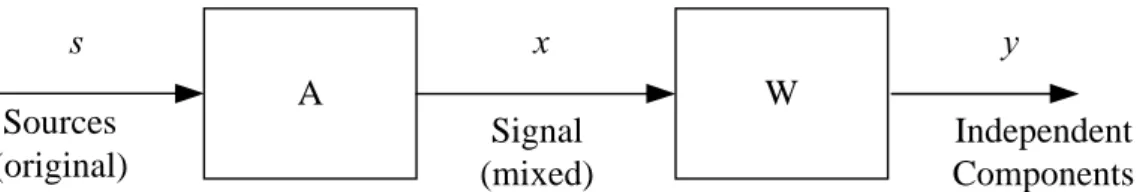
(17) (a) The mixtures of original signals. (b) The original signals Figure 2. The original signals and its mixtures As far as the stock market is concerned, the stock price is a mixture signal as if the sound picked by the microphone. The effect factors of stock price, such as politics, exchange rate, and economics (section 2.1), are similar as the speakers in the room. The stock price will be varied according to the happening sequence and the degree of the effect factors. In this thesis, ICA is used to find out the independent components from price volatility, even though the meaning of them cannot be known.. 2.2.2 Independent Component Analysis. The basic process of ICA is shown in Figure 3, where the symbol x represents the mixture signal, and s refers to the original one. The mixture signal x is computed as the equation (3) or (4).. 8.

(18) x. s Sources (original). y. A. W Signal (mixed). Independent Components. Figure 3. The basic procedure of ICA. n. xi (t ) = ∑ aij s j (t ). (3). x = As. (4). j =1. In equation (3), {xi(t)}, i = 1,2,…,n, contains n mixture signals and t is the time step. In equation (4), A (aij) is a n × n mixing matrix, which describes the mixing process. In equation (5) and (6) that are listed in the following statement, y(t) is the independent component. The problem is to compute a de-mixing matrix W such that. y (t ) = Wx(t ). (5). y (t ) = WAs(t ). (6). Independent components, y(t), are latent or hidden factors which can not be obtained by direct observation or measurement. Matrix A, as described above, is an unknown mixing matrix. ICA enables the mixture signal x to estimate the mixing matrix A and the original signal s. There are two fundamental assumptions related to ICA [1]. Firstly, the original sources {sj(t)} must be statistically independent. Secondly, the original sources {sj(t)} should not be Gaussian distributions, and at most only one is permitted to follow a Gaussian distribution. Two random variable s1 and s2 are independent if the information of s2 can not be inferred from s1, and vice versa. For each two measurable functions h1 and h2 can be obtained, as shown in equation (7).. 9.

(19) E{h1 ( s1 )h2 ( s2 )} = E{h1 ( s1 )}E{h2 ( s2 )}. (7). There are still other approaches of ICA estimation, including maximization of nongaussianity, maximum likelihood estimation, and minimization of mutual information that can be studied for the future work.. 2.2.3 Preprocessing for Independent Component Analysis. Before using ICA method, two preprocessing techniques are required to make the problem in better condition. The preprocessing work involves two procedures, centering and whitening. Centering is the variable that subtracts the mean vector from x, which is called zero-mean method, as shown in equation (8). ^. x = x − E{x}. (8). ^. In equation (8), x represents the outcome of the centering. E{x} is mean vector of x. ^. The second step is whitening, which translates x into white noise. The purpose of whitening is to eliminate the correlation among the data. Whitening vector enables the observed signals to be non-correlated for making the variance of them to be one. Whitening refers to the ^. covariance matrix of x , and it is an identity matrix, which is shown as equation (9).. (9). ~. x = ED −1 / 2 E T x. In equation (9), E is eigenvectors of covariance matrix E{xxT}. D is eigenvalue. The ~. covariance matrix x is identity matrix in equation (10). ~ ~T. E{x x } = I. (10) 10.

(20) 2.2.4 Application. The most popular application of ICA is cocktail-party problem. In medical science, ICA is used to analyze magnetoencephalography (MEG) data, which is a technique for recording the magnetic activity in the brain. In the finance domain, Back and Weigend (1997) [4] applied ICA to extract the structure from stock price change. In addition, ICA is also suitable for reducing the noise in natural images. In telecommunications, ICA is applied to separate the user’s own signal from other mixtures in CDMA (Code Division Multiple Access). In the thesis, ICA is applied for reducing noise of stock price.. 2.3 Pattern Recognition for Time Series Time series is a sequence that associated with time. A lot of research has been done on the time series analysis and forecasting [18][24], such as stock price prediction, temperature forecasting, sales, traffic flow statistics, and so on. Last et al. (2001) [24] define that the time series consists of static and dynamic attributes. For example, in stock market database, the company name and the corresponding symbol are part of static attributes, while the dynamic attributes involve daily closing price and trading volume. Furthermore, the dynamic attributes are closely related to the time, and some of them are mutually dependent.. Pattern recognition is a branch of artificial intelligence. It is used to classify the objects and patterns based on prior knowledge or statistics of source data. The features of an object include the form, color, size, and shape. The main applications of pattern recognition are speech recognition, fingerprint, object detection, face recognition, and so forth. In a pattern recognition model, the sensor is used to collect the observed information for classifying and describing the significant features. Therefore, feature extraction is the underlying mechanism, which contributes to the incorporate the external information in a flexible way. 11.

(21) Pattern recognition, as described above, is suitable for time series data mining. Keogh and Kasetty (2002) [11] categorize the time series mining into four types, which are introduced as follows.. (1) Indexing: Firstly, a known sequence and a similar measurement function are given. The purpose of indexing is to find out the most similar patterns from the large data sequence. (2) Segmentation: Assume that a given time series Q contains n data points. The objective of segmentation is to discover k points among the time series (k<<n) for setting up a new model Q’. As a result, the model Q’ can be a representative for approximating the original time series Q. (3) Clustering: Clustering is an unsupervised learning technique. It groups the observed patterns or data into classes without priori knowledge. By giving some time series data and similar measurement functions in advance, the clustering algorithm will automatically group by similarity. (4) Classification: Classification is a supervised learning technique that the known sequences or patterns are given in advance. The pattern will then be classified into different categories according to the presented information.. The indexing, segmentation, clustering, and classification techniques in time series as mentioned above, will be detailed discussed in the following sections.. 2.3.1 Indexing. Chu and Wong (1999) [20], and Man and Wong (2001) [26] propose an indexing approach which does the scaling, and transformation on time series. The purpose of this method is to match the most similar pattern between the query sequence and historical ones. Suppose (qxi,qyi) represents the pattern of a sequence, and (cxi,cyi) is the most similar pattern 12.

(22) that needs to be discovered. The query pattern (cxi,cyi) must be translated by the scaling and translation matrix. The proposed scaling method is used to transform the size of the query pattern for fitting the historical one; otherwise, the historical pattern will be converted to fit in with the query one. The transformation refers to the horizontal and vertical shift from the historical pattern to the query one.. Rafiei and Mendelzon (2000) [10] show that Euclidean distance and city-block distance are the two most common approaches for similarity matching. However, the complex pattern can not be easily presented by the distance-based measures. Hence, the data for pattern matching needs to be transformed into another type. Accordingly, the authors propose the single and multiple transformation methods, including time scaling, moving average, time shift, and Discrete Fourier Transform (DFT). They also show that the transformation will not destroy the characteristics or structures of the original data. Distance based pattern matching method compares the same length time series and it is not suitable for discovering stock trend pattern.. Dynamic time warping (DTW) is one of the most popular methods for time series pattern matching and speech recognition (Chen et al. 2001) [13] DTW can do the matching with the corresponding peak and valley dynamically and precisely, regardless of the time lag. Nevertheless, DTW is time-consuming, and the performance will downgrade if the difference of two sequences is too large that the relative high and low do not match.. Yang et al. (2003) [17] propose an elastic model to find out the asynchronous periodic patterns. Two parameters min_rep and max_dis are used to discover the valid patterns. The frequency of the valid patterns must be at least min_rep times of appearance of continuous subsequence, and the length of disturbance between the neighboring subsequences should be less than max_dis. This model can find periodic pattern and omit disturbance, which is 13.

(23) suitable for web access log mining.. Chiu et al. (2003) [9] apply a random projection algorithm to discover the significant patterns. In projection algorithm, the dimension of a sequence must be reduced greatly. Firstly, the time series will be symbolized, which means that the time series of dimension n will be translated into w-dimensional space by each mean (w<<n). The values n and w are defined by the application and demand. The time series is encoded into symbolic form and stored in the matrix. Secondly, the random projection algorithm will be applied to select the columns randomly for mask matching. Thirdly, the identical patterns in the mask will be recorded in the collision matrix. After reiterating the procedures for suitable number of times, the collision matrix must be checked to observe the cells with higher value. The cells with greater value do not guarantee for the significant patterns; however, it is an evident signal of having more opportunities to discover valuable patterns. As a result, the original data of these cells must be fetched for further analysis.. Povinelli and Feng (2003) [27] propose a pattern identification method. They define an event characteristic function g(.) to describe the happenings in time series data. Firstly, a temporal pattern, which is the event characteristic function, is defined. The objective of the approach is to predict the events rather than doing the prediction on the whole time series. Simple genetic algorithms will then be used to search for the optimal temporal pattern based on the application problem.. Kahveci and Singh (2004) [35] propose an indexing structure to store multi- resolution patterns, called Multi-Resolution (MR) index structure. Discrete Fourier Transform (DFT) or wavelet will then be used to translate the time series data into the length of base 2, and store in the MR index structure. The improved algorithms, range query and nearest neighbor query, enable the parallel implementation as presented by the authors. 14.

(24) 2.3.2 Segmentation. Guralnik and Srivastava (1999) [37] define the change points to show the direction change in the time series, where the change points represent the events in the time sequence. The number of change points is decided in accordance with two steps that are stated as follows. Firstly, the number of change points needs to be determined in advance. Secondly, a function will be used for curve fitting among the change points. The time series will be divided into several segments which are represented by the fitting function. The likelihood criterion will then be applied to verify whether the segments should be separated or not. The stopping criterion is that the likelihood will not change a lot even though more change points are added.. Ge and Smyth (2000) [42] apply segmentation Markov model to divide the time series into several subsequences. Each subsequence is described by a parametric function. And this model deals with plasma etch process in semiconductor manufacturing.. Man and Wong (2001) [26] propose a method to identify the important peak and valley points in the time series. The relative high and low points, namely control points, can describe the critical changes in the time series. The control points, either local maximum or local minimum, must be sorted based on the level of significance. The importance refers to the change direction. The control points will then be stored in the lattice structure after being sorted.. Park et al. (2001) [32] propose a segment-based approach for subsequence matching in time series. The time series is divided into several segments, and each of them is a monotonically changing pattern. They will be either monotonically increasing or monotonically decreasing patterns. After the segmentation procedure, feature extraction will. 15.

(25) then be done for similarity matching.. 2.3.3 Clustering and Classification. Clustering is an unsupervised learning that groups the patterns or data into several classes or groups. The elements in the same cluster are more similar to one another than they are in separate ones.. Ralambondrainy (1995) [14] proposes a new method that extends from K-means clustering algorithm to deal with the hybrid numeric-symbolic computation of a clustering problem. Clustering algorithms include two procedures. The first step is to group the data into several classes automatically. The second one is to analyze the characteristics of the data within each class. Euclidean distance measurement is suitable for numeric data but not for symbolic data. The symbolic data must be transformed into numeric data with finite possibilities. For example, the gender attribute {male, female} can be translated into the values {1, 2}. Euclidean distance can be applied to symbolic data after the translation procedure. But the distance is based on the number of possible value.. Classification is a supervised learning method that the known patterns of each class are given previously. Petridis and Kehagias (1996) [38] combine two modular design methods, Bayesian statistics and partition algorithm, to do the classification in the time series. The partition algorithm is implemented by neural network with recursive processes of off-line and on-line learning. The off-line learning phase is used to build a predictor module for training the time series data. The error between the prediction and the actual observation will then be individually computed to update the posterior probability of the time series data. The credit will be appointed to each predictor based on neural network, which is regarded as an on-line process. Partition algorithm can be parallel implemented to reduce the execution time. 16.

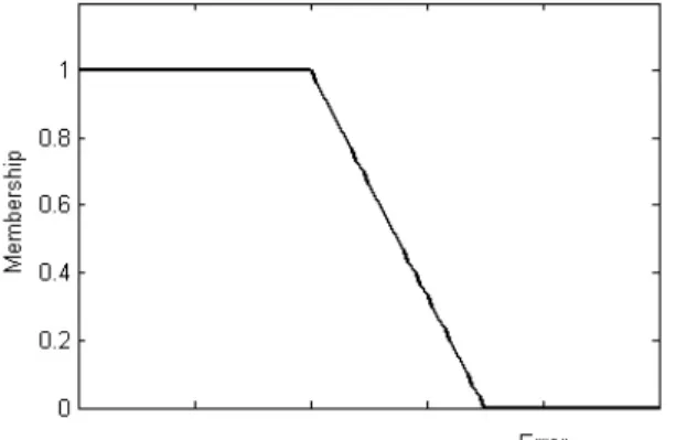
(26) substantially and do the piecewise training flexibly.. Jain et al. (1999) [6] give a review on clustering techniques. Several clustering approaches have been proposed, such as hierarchical clustering algorithm, partition algorithm, mixture-resolving and mode-seeking algorithm, nearest neighbor clustering, fuzzy clustering, and some artificial intelligence models.. Han and Kamber (2001) [16] introduce the concept of classification which is a supervised learning for categorizing data into several given classes. Some classification techniques have been presented, such as decision tree, Bayesian classification, neural network, and other evolution approaches. The classification model contains two procedures. In the first step, the training data is used to build a model according to the classification algorithm. Next, the testing data will be used for validation and testing the accuracy of the model.. 2.4 Fuzzy Set Theory Fuzzy set has been used popularly in the controlled system and pattern recognition domains. Zadeh (1965) [22] proposes the concept of fuzzy set which is the extension of crisp set. In the crisp set, an element either is enclosed in or does not belong to one set. In real world, the crisp set is unable to explain the complex phenomena of the environment clearly. For example, define the temperature of more than 30o belongs to the class “hot”. However, the temperature of 29.5o that is 0.5o lower does not match “hot”. The classification method on the temperature is not reasonable enough. Nevertheless, fuzzy set theory can distinguish different degrees of membership in a set. The membership function is used to express to what degree a value belongs in the interval [0, 1] in a set. There are several common types of membership function [19][21], such as triangular, trapezoidal, bell, and Gaussian that are shown in Figure 4. The horizontal axis represents an observation (i.e. warm temperature). The vertical axis. 17.

(27) illustrates the degree of membership value between 0 and 1.. (a) Triangular MF. (b) Trapezoidal MF. (c) Bell MF. (d) Gaussian MF. Figure 4. Four basic classes membership function. Figure 5. The membership function of matching error. 18.

(28) In the thesis, the concept of fuzzy set is used to represent the degree of similarity between two matching patterns (see Figure 5). The higher the error represents the lower the similarity, which leads to the smaller value of membership function. On the contrary, a greater value of membership function corresponds to the smaller error and higher similarity.. 19.

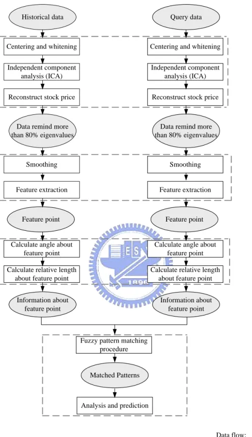
(29) Chapter 3 System Architecture In the thesis, the experimental data is collected from Securities & Futures Institute (SFI). The simulation approaches are stated in the following. Firstly, independent component analysis (ICA) is applied to discover the independent components (ICs) of the stock price. The dominated ICs will then be used to reconstruct the stock price. Secondly, feature extraction will be applied to the daily closing price data based on the perceptually important points. Thirdly, the angle and relative length are computed for matching similar patterns, namely the resembling stock price trend. Finally, the investment suggestions will be given according to the analysis result. The procedures of the above-mentioned approaches are illustrated in Figure 6.. 3.1 Reducing Noise in Stock Price. 3.1.1 Objective. The stock price is reflected by many factors, such as politics, economics, international statuses, significant news, and so on. The stock price is final result that be regarded as a mixture signal of the stock market. The degree of effect results from each of the factors is quite different; some are important that may happen at the right time infrequently, but some are weak that occur with high frequencies. ICA is capable of discovering the independent components or hidden patterns in the stock price. Although the real meaning of each ICs cannot be interpreted, the degree of explanation of the stock price can be known individually. Therefore, each ICs will be sorted in descending order by the level of explanation (eigenvalue). The objective of applying this method is to retain the important and dominant. 20.

(30) Historical data. Query data. Centering and whitening. Centering and whitening. Independent component analysis (ICA). Independent component analysis (ICA). Reconstruct stock price. Reconstruct stock price. Data remind more than 80% eigenvalues. Data remind more than 80% eigenvalues. Smoothing. Smoothing. Feature extraction. Feature extraction. Feature point. Feature point. Calculate angle about feature point. Calculate angle about feature point. Calculate relative length about feature point. Calculate relative length about feature point. Information about feature point. Information about feature point. Reducing noise. Feature extraction. Information for matching. Fuzzy pattern matching procedure. Pattern matching. Matched Patterns. Analysis and prediction. Data flow:. Methodology:. Figure 6. The procedure of approach 21.

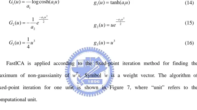
(31) components for reconstructing the new “stock price”.. 3.1.2 Fast Independent Component Analysis. In this thesis, fast independent component analysis (FastICA) [2] is applied to find the independent components (ICs) of the stocks, and eliminate the ICs with lower contribution. FastICA has been proved to be quite efficient for finding the ICs. The input data has to be firstly preprocessed through centering and whitening that has been described in section 2.2.3. The main objective of FastICA is to maximize the “negentropy”. Here, the concept of entropy, which represents the measurement of uncertainty, will be used. The higher the value of entropy, the more disordered the data content. The entropy H is showed as equation (11), where symbol y is a random variable. H ( y ) = − ∫ f ( y ) log f ( y )dy. (11). Besides, the entropy can be used as a measurement for non-gaussianity. Define J as negentropy as shown in equation (12), which is modified by equation (11).. J ( y ) = H ( y gauss ) − H ( y ). (12). The variable ygauss is a Gaussian random variable, whose covariance matrix is the same with the variable y. Gaussian random variable has the largest entropy value, therefore negentropy is always positive. Negentropy is zero when y is Gaussian random variable. Negentropy is usually regarded as a measure of non-gaussianity. Because it is difficult to compute negentropy; the estimation of probability density function (p.d.f) must be known in advance. Therefore, the approximation of negentropy is developed as shown in equation (13). In equation (13), symbol v is a standardized Gaussian variable with zero mean and unit variance. Symbol y is a variable with zero mean and unit variance, and G is a non-quadratic 22.

(32) function. J ( y ) ∝ [ E{G ( y )} − E{G (v)}]2. (13). Hyvärinen (1999) [2] shows three basic forms of G and their corresponding derivatives g as listed in equation (14), (15) and (16), where 1≦a1≦2 (usually selected as the value 1) and a2 ≈ 1. G1 can be used in general purpose applications; hence, it is applied in this thesis. G1 (u ) =. 1 log cosh(a1u ) a1. 1 G2 (u ) = − e a2. − a2u 2 2. g1 (u ) = tanh(a1u ). g 2 (u ) = ue. 1 G3 (u ) = u 3 4. −a2u 2 2. g3 (u ) = u 3. (14). (15). (16). FastICA is applied according to the fixed-point iteration method for finding the maximum of non-gaussianity of wTx. Symbol w is a weight vector. The algorithm of fixed-point iteration for one unit is shown in Figure 7, where “unit” refers to the computational unit.. Fixed-point Algorthim for one unit Input : mixture signal after centering and whitening Output: Independent component Choose an initial weight vector w randomly While not convergence w+ = E{xg ( wT x)} − E{g ' ( wT x)}w w=. w+ w+. end Figure 7. Fixed-point algorithm for one unit. 23.

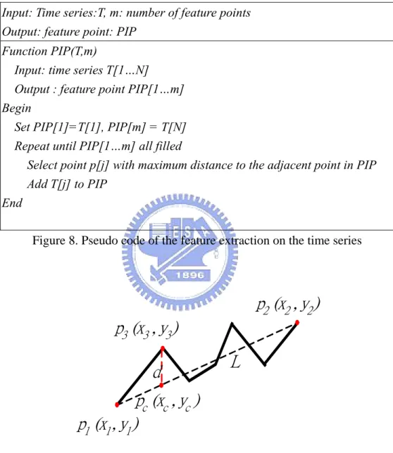
(33) The stop criterion indicates that the old and new w parallel converge in the same direction, which the dot product equals 1. There is only one independent component (IC) can be found by using fixed-point algorithm for one unit. FastICA algorithm can find several ICs based on fixed-point algorithm for one unit. The relationship of the weight vectors w1,w2,…,wn must be decorrelated after every iteration. That can prohibit from converging in the same maximum.. 3.2 Feature Extraction Feature extraction is a technique that discovers the characteristics of source data. The method of perceptually important points (PIPs) [12] [15] is applied to discover the most important points in the handwritten signature and time series. The steps of feature extraction proposed in this thesis, based on the pseudo code in Figure 8, are stated as follow. Step 1: The first two feature points the start point p1 and the end point p2, are determined (see Figure 9). Step 2: In Figure 9, the line connecting p1 and p2, namely L, will then be drawn. Every point on the time series must be checked for their vertical distances to L. The vertical distance d is calculated base equation (17). The point with the maximum vertical distance will be selected as the next feature point. For example, in Figure 9, p3 has the maximum vertical distance from L between p1 and p2. Thus, p3 is chosen as a feature point followed by p1 and p2.. d = |yc-y3| = y1 +. ( y2 − y1 )( xc − x1 ) − y3 x2 − x1. (17). Step 3: The adjacent feature points are connected with each other. For instance, the point p1 is connected to p3, and p3 is connected to p2. The process will be iterated continuously to 24.

(34) find the points with the maximum vertical distance from the connecting line between the adjacent feature points. The loop will be not stopped until finding enough predefined feature points.. Input: Time series:T, m: number of feature points Output: feature point: PIP Function PIP(T,m) Input: time series T[1…N] Output : feature point PIP[1…m] Begin Set PIP[1]=T[1], PIP[m] = T[N] Repeat until PIP[1…m] all filled Select point p[j] with maximum distance to the adjacent point in PIP Add T[j] to PIP End Figure 8. Pseudo code of the feature extraction on the time series. p2 (x2 , y2 ) p3 (x3 , y3 ) L. d pc (xc , yc ) p1 (x1 , y1 ). Figure 9. Time series of feature extraction. The proof of equation (17) is detailed described in the following. There are 8 cases for finding the feature points in the time series, which are illustrated in Figure 10 (a) to (h). Take Case 1 for example: ΔP1Pc a ≅ ΔP1P2 b. (18) 25.

(35) xc − x1 yc − y1 = x2 − x1 y2 − y1. (19). xc − x1 ( y3 − y1 ) − d = x2 − x1 y2 − y1. (20). ∴. d= y1 +. ( y2 − y1 )( xc − x1 ) − y3 x2 − x1. (21). Likewise, the other seven cases can be proved by equation (17).. p2 (x2 , y2 ) p3 (x3 , y3 ) pc (xc , yc ). pc (xc , yc ) L. L. d. d. a. p1 (x1 , y1 ). b. (a) Case 1. p1 (x1 , y1 ). b. a. L. L. p2 (x2 , y2 ). p2 (x2 , y2 ). (c) Case 3. (d) Case 4. pc (xc , yc ). p3 (x3 , y3 ). p1 (x1 , y1 ). d pc (xc , yc ). p3 (x3 , y3 ). d. L. p2 (x2 , y2 ) p (x , y ) 1 1 1. L. p3 (x3 , y3 ). (e) Case 5. (f) Case 6. pc (xc , yc ). L. p2 (x2 , y2 ) d. p2 (x2 , y2 ). d. pc (xc , yc ). p1 (x1 , y1 ). b. p3 (x3 , y3 ). pc (xc , yc ). d. b. (b) Case 2. a. p1 (x1 , y1 ). p3 (x3 , y3 ). a. p1 (x1 , y1 ). p2 (x2 , y2 ). L. p1 (x1 , y1 ). d. pc (xc , yc ) p3 (x3 , y3 ). p3 (x3 , y3 ). (h) Case 8. (g) Case 7. Figure 10. 8 cases when finding feature point in time series. 26. p2 (x2 , y2 ).

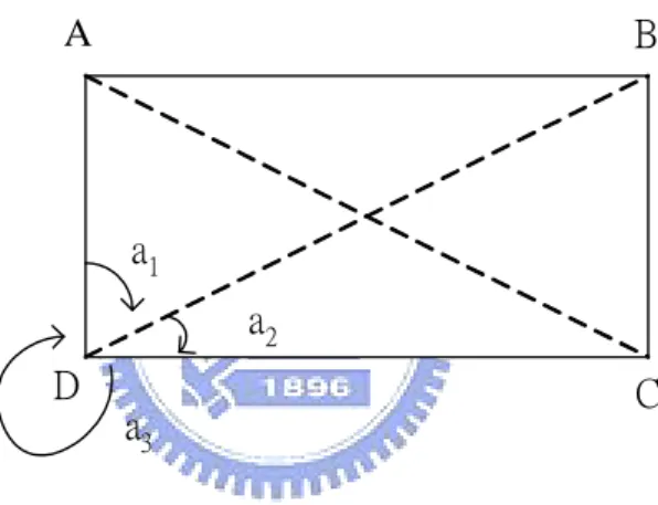
(36) 3.3 The Information about Adjacent Feature Points After feature extraction, some information about the adjacent feature points must be computed, including the angle and relative length. Thus, the similar patterns in the time series could be discovered through the computed information. Auwatanamongkol (2000) [34] propose a similarity measure that is necessary for doing the matching on a 2D object pattern. The essential condition is called angle. In Figure 11, the angles of rotation (a1, a2, a3) are the matching criterion. The advantage of angle matching is that the angle will not be affected regardless of the rotation or scaling of an object. B. A. a1 a2 D. C. a3. Figure 11. 2D pattern matching. 3.3.1 The Angle of Adjacent Feature Points. In order to compute the angle of the adjacent feature points, the slope of any two of them needs to be firstly calculated. Slope matching is quite complicated because the slope lies within the range [- ∞ , ∞ ]. Therefore, the first step is to convert the slope into the angle, as shown in the equation (22), where the symbol S represents the slope and α is the corresponding angle. The second step is to use the angle to do the matching.. α=. tan −1 S × 180o. (22). π 27.

(37) There are two characteristics of angle matching:. (1) Normalization is required for the angle matching in financial applications. That is because different angles can be formed by the identical stock volatility. For example, two different stocks A and B rise 10 percent from 10 to 11 and from 50 to 55 respectively. According to the concept of normalization, the points of A should be multiplied by five; otherwise the points of B ought to be divided by five. (2) The similar patterns of arbitrary lengths can be discovered through angle matching. The reason is that there is no impact on two angles regardless of the time length. As long as the number of the chosen feature points is equal, the M-day data is capable of being matched with N-day data. For instance, the data of 50 days can be matched with 60 days An error rangeεshould be predetermined when doing the matching process, and the angle needs to be lied within the range [-90o, 90o]. In this experiment, α denotes the angle of a feature point; therefore, α ± εare regarded as the identical angles. Furthermore, the smaller the error rangeεis, the more precise the matching results will be. On the other hand, the bigger the error range, more similar patterns can be discovered.. 3.3.2 The Relative Length of Adjacent Feature Points. The time interval of two feature points may differ in various patterns. As far as the stock data is concerned, different patterns on different time periods imply diverse meanings. Therefore, the horizontal distance of the adjacent feature points should be taken into consideration when doing the matching process. In order to flexibly compare different lengths of time series, the relative time length is used as a measure. The time length of adjacent feature points divided by the total length of the time series equals to the relative length. For instance, in Figure 12, the total length is N, and a1 , a 2 ,..., a n are its segments. As a result, the 28.

(38) relative length of each segment is. a1 a2 a , ,..., n . N N N. X a1. a2. a3. an. N. Figure 12. The relative length of adjacent feature points. 3.4 Similarity Matching As mentioned above, the process of matching begins with discovering the most critical feature points based on the feature extraction method. Next, the angle and relative length of the adjacent feature points will be calculated, which are described in section 3.3.1 and 3.3.2. The angle is computed as shown in equation (23). The symbol Ai and Bi stand for the angles of time series X1 and X2 respectively, andεis the error of the angle. The character i is an index of adjacent feature points. In Figure 13, X1 and X2 are two time series, and the red dots represent the feature points. | Ai − Bi | < ε 1 Ai × Bi ≧0. (23). n: number of feature points. 29.

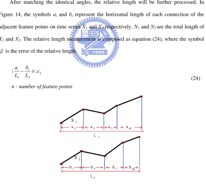
(39) A2. AN. X1. A3 A1. BN. B2 B3. X2. B1. Figure 13. The first similarity measurement, angle After matching the identical angles, the relative length will be further processed. In Figure 14, the symbols ai and bi represent the horizontal length of each connection of the adjacent feature points on time series X1 and X2 respectively. N1 and N2 are the total length of X1 and X2. The relative length measurement is computed as equation (24), where the symbol β is the error of the relative length.. |. ai bi − |< ε 2 L1 L2. (24). n : number of feature points. X. 1. a2. a1. L. X b1. a n1. a3 1. 2. b2. b3. b n2. L2. Figure 14. The second similarity measurement, relative length. 30.

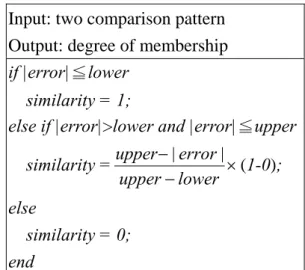
(40) The matching patterns may be dissimilar even with the identical angle; that is why the relative length needs to be matched. The error of the angle and relative length requires being falling into the range of tolerance; thereupon, the matching results will be regarded as identical. The stricter the matching conditions, the better results will be displayed; contrarily, the fewer identical patterns will be matched if the related condition is loose.. 3.5 Trend Analysis After matching the similar curves, the trend for the subsequent n days will be analyzed. Since the similarities of patterns are in different degrees, the fuzzy logic is then applied to deal with different degrees of the data. A membership function (MF) describes the linguistic values in terms of numerals, which varies from 0 to 1.. In the thesis, fuzzy logic is used to indicate the degree of similarity between two patterns. The membership function of the similarity is shown in Figure 15. If the matching error is less than lower, the membership function is set 1. If the matching error is less than upper and greater than lower, the membership function is between 0 and 1. Otherwise, membership function is set 0. The pseudo code of the MF is shown in Figure 16.. Degree 1 of Similarity 0. lower. upper error. Figure 15. The membership function of similarity. 31.

(41) Input: two comparison pattern Output: degree of membership if |error|≦lower similarity = 1; else if |error|>lower and |error|≦upper similarity =. upper − | error | × (1-0); upper − lower. else similarity = 0; end Figure 16. The pseudo code of membership function. The future trend will be analyzed after matching the curve (see Figure 17). The effective price limits (γi) are computed as showed in equation (25). The symbol ‘pe’, ‘l’, ’h’ represent the trading price at the beginning date, the lowest price and the highest price of the subsequent n days respectively. The effective price limits ( γ i) of each matching pattern must be computed by the weighted average method. The weighted average of the effective price limits,. γw, is thus formed as shown in equation (26). For example, there are three fundamental trading strategies as listed in Table 1, where γ t is the trend threshold. In Figure 17, the pattern ‘papbpcpdpe’ is uptrend if γw is greater than the specified threshold γt. On the other hand, the pattern ‘papbpcpdpe’ is downtrend ifγw is smaller thanγt. Otherwise, the subsequent trend of the matching pattern cannot be determined. Accordingly, the corresponding future trend of a certain pattern is capable of being decided by above-mentioned approaches.. 32.

(42) Price. pd. h. pe. l. pb n. pc. pa. Now. Future. Time. Figure 17. The valid price fluctuation rate figure. γi =. hi − li ei. (25). n. γw =. ∑ (similarity × γ ) i. i =1. i. n. ∑ similarity i =1. (26). i. n: number of matching patterns Table 1. Trading strategies. γ t is the trend threshold. γ w is the weighted average of the effective price limits Condition γw ≥γt. γ w ≤ −γ t −γt < γw < γt. Trading strategy To buy stock at beginning date and sell out at the end date To do short at the beginning date and buy at the end date Not trading. 33.

(43) Chapter 4 Simulation 4.1 Data Description The daily closing price of the weighted-value stocks in Taiwan Stock Exchange (TAIEX) is fetched from Securities & Futures Institute (SFI). Besides, data of the electronic stocks that contains more than 1,500 trading days are selected. There are fourteen stocks that are chosen for the simulation as listed in Table 2. The total time period of the experimental data begins from November 26th, 1996 to April 28th, 2004. Accordingly, the data from November 26th, 1996 to December 31, 2001 is regarded as the historical dataset for 1,367 trading days. Subsequently, the data from January 1st, 2002 to April 28th, 2004 is the testing set for the matching work. Table 2. Fourteen value-weighted stocks of the electronic industry in TAIEX (Recorded on 2004/4/30) ID. Symbol. Company name. Weighted-value. 2330. TSMC. Taiwan Semiconductor Manufacturing Co., Ltd.. 8.71%. 2303. UMC. United Microelectronics Co.. 3.59%. 2317. Hon Hai. Hon Hai Precision Ind. Co., Ltd.. 2.70%. 2357. Asustek. Asustek Computer Inc.. 1.21%. 2324. Compal. Compal Electronics, Inc.. 0.90%. 2311. ASE. Advanced Semiconductor Engineering, Inc.. 0.73%. 2352. Benq. Benq Corporation.. 0.72%. 2353. Acer. Acer Incorporated. 0.72%. 2323. CMC. CMC Magnetics Corporation. 0.66%. 2301. Lite-On. Lite-On Electronics, Inc.. 0.58%. 2344. WEC. Winbond Electroincs Corp.. 0.57%. 2337. MXIC. Macronix International Co., Ltd.. 0.48%. 2308. Delta. Delta Electronics, Inc.. 0.45%. 2325. SPIL. Siliconware Precision Industries Co., Ltd.. 0.41%. 34.

(44) 4.2 Model Parameters The model parameters that will be used are described as follows.. Number of dominant ICs [4]: The number of domination ICs to be retained depends on the capability of explaining the stock. Back and Weigend (1997) [4] state that only a few ICs provide the greatest change in the stock price fluctuation. The dominant ICs represent the major level change, and the non-dominant ICs express the minor level change. In the research, the independent components that can explain more than 80% of the stock will be kept for reestablishing the stock price. Consequently, 8 ICs with the highest eigen values are selected as the representatives in this model. Number of feature points: Levy (1971) [29] used significance five-point chart pattern to forecast the future trend of stock price. In this thesis, the number of feature points is also determined in advance. The display of different number of feature points, from 2 to 7, is shown in Figure 18. The number of feature points versus the average error is calculated from 100 patterns, illustrated in Figure 19. The average error equals to the absolute value of solid line minus dotted line of Figure 18. The number of feature points is based on the domain application. Accordingly, 6 feature points are more suitable for the simulation in this thesis. Comparison days and prediction days: Comparison days refer to the data in the matching curve, while the prediction days are the subsequent days followed by the matching curve. They are defined by means of trial-and-error. In this experiment, the strategy focuses on the mid-long term that the comparison-day is 60 days and the prediction-day is 20 days. Matching criteria: The angle error and the relative length of the feature points are the matching conditions. The fuzzy set concept is introduced.. 35.

(45) Average error. Figure 18. Different number of feature points, which are 2, 3, 4, 5, 6, and 7 are showed. The solid lines are original stock price. The squares are feature points. The dotted lines are the links between adjacent feature points.. 10 8 6 4 2 0 2. 3. 4. 5. 6. 7. Number of feature point. Figure 19. The number of feature points and average error. 4.3 Independent Component Analysis The stock price p(t) should be transformed into the form of the price change x(t ) = p(t ) − p (t − 1) or the geometric growth x(t ) = log( p (t )) − log( p(t )) before using ICA (Back and Weigend, 1997 [4]). Symbol t is time stamp. However, in this simulation, the ratio concept should be applied to the fourteen simulated stocks due to the different scale of stock price levels, which is listed as equation (26). x(t ) =. p(t ) − p(t − 1) P(t − 1). (26). There are at most fourteen independent components (ICs) will be found from the fourteen input stocks. The eigenvalues of the fourteen ICs are calculated and sorted in descent 36.

(46) order (see Figure 20). The dominant ICs will be retained for reconstructing the stock price. Nevertheless, the ICs with small eigenvalues will be ignored as the noise. In the research, the eight dominant ICs that are kept can express more than 82.78% of the stock price fluctuation, which are shown in Figure 21. And the reconstruction pattern of the stock ‘TSMC’ by the eight dominant ICs is illustrated in Figure 22.. 0.009 0.008 0.007 0.006 0.005 0.004 0.003 0.002 0.001 0 1. 2. 3. 4. 5. 6. 7. 8. 9. 10. 11. 12. 13. Figure 20. The ordering eigenvalues. Figure 21. Eight dominate independent component. 37. 14.

(47) Figure 22. The reconstruction stock price. The dished line at the top is the original stock price of TSMC. The solid line is reconstruction stock price by the eight dominant ICs. The dotted line at the bottom is the pattern reconstructing by the remaining six ICs.. 4.4 Data Normalization The weight moving average (MA) method is used to smooth the trend of TAIEX stock price, as shown in equation (27). The purpose of smoothing is to reduce the fluctuation for finding out the most important points by feature extraction. In the simulation, 5-days weight MA is used to smooth time series. n. mat =. ∑i ×T. t − ( n −i ). i =1. (27). n. ∑i i =1. T: time series t: today, n: days average. After the smoothing process, the normalization for pattern matching will be implemented. Generally, the typical form of normalization (Rafiei and Mendelzon, 2000) [10] is listed as. 38.

(48) equation (28). The time series X = {x1 , x2 ,..., xn } shifts by its mean and divides by its standard deviation. X = {x1 , x2 ,..., xn } is translated into X * = {x1* , x2* ,..., xn* } . This smoothing method is suitable for the distance-based matching, while a scaling method is fitting for the angle matching. If there are two sequences X 1 = {a1 , a2 ,..., an } and X 2 = {b1 , b2 ,..., bn } for matching, X2 must be multiplied by. a1 . For example, X1= {100, 90, 99} and X2= {200, 180, b1. 198} both fall 10% then rise 10% during the same time period, but the angles of the sequences may differ. Therefore, X2 must be multiplied by. 100 1 = , such that X2*={100,90,99} in 200 2. equation (29).. xi* =. xi − mean( X ) , 1≦i<n std ( X ). (28). n: number of the time series std: standard deviation. X 2* =. a1 × X2 b1. (29). Two time series: X1 ={a1,a2,…,an}, X2 ={b1,b2,…,bn}. 4.5 Pattern Matching and Analysis After smoothing and normalization processes, the feature extraction method will be applied to discover the feature points for storing in the feature vector. The stock price of UMC from June 20th, 2002 to September 26th, 2002 is an example shown in Figure 23. The information about the feature points, which includes angle and relative length, is calculated to store in the feature vector as shown in the tables of Figure 23. The time refers to the experimental time period, and the value is the corresponding stock price.. 39.

(49) After the matching procedures, the matching patterns will be analyzed by the weighted average γ w as stated in equation (30). The effective price limits γ i is described in section 3.5. The symbol similarity1 and similarity2 represent angle error and relative length error respectively. Their membership functions are illustrated in Figure 24 and 25. The first membership function describes the similarity by angle error. The up-trend and down-trend are eight degree in this thesis, therefore the upper bound of angle error is 90/8 = 11.25. The second membership function defines the similarity by relative length error. In this thesis, six feature points are used, have five segments of adjacent feature points. Each segment is 20% of total length. Therefore, the maximum toleration of relative length error is a half of length of segment (10%).. Value Time Angle. 62.4 66.1 53.6 51.4 55.6 48.0 1. 16. 35. 45. 51. 60. 14.4021 -45.0313-12.5319 49.4872 -71.7436. Relative length 0.2500 0.3167 0.1667 0.1000 0.1500 Figure 23. The stock price of UMC is for feature extraction. The squares are feature point. The solid line represents original stock price. The dotted line shows the link between adjacent feature points. The light solid line is 5-days moving average.. 40.

(50) n. γw =. ∑ (similarity. 1i. i =1. × 0.5 + similarity2i × 0.5) × γ i. n. ∑ (similarity i =1. 1i. (30). + similarity2i ). Degree 1 of Similarity1 0. 6. 11.25 Angle error. Figure 24. The first membership function of similarity. Degree 1 of Similarity2 0. 0.05. 0.1. Relative length error. Figure 25. The second membership function of similarity The patterns contained ex-dividend stocks must be ignored because the stock price will drop on the ex-dividend day. Therefore, the stock price needs to be adjusted. The maximum daily price fluctuation limit is set 7% in Taiwan stock market. Hence, the patterns must be eliminated when the daily price fluctuation is more than defined limit. In the prediction process, the profit rate (pr) is predefined (see Figure 26). Thus, five trading strategies are displayed in Table 3.. 41.

(51) Price. pd. p e × (1+. pr ). pe pb. pa. p e × (1-. pr ). n. pc. Now. Future. Time. Figure 26. The concept of the profit rate. Table 3. The trading strategies Model. Condition. Beginning date. End date. prediction If the stock price is greater than pe×(1+pr), the stock can be sold earlier for obtaining pe × pr. γw ≥γt. profit. Up-trend. Buy stock at pe If. the. stock. price. is. not. greater. than pe × (1 + pr ) , the stock will not be sold until the specified end date. If the stock price is less than pe × (1 + pr ) , the stock can be bought earlier for obtaining. γ w ≤ −γ t. Down-trend. Short at pe. pe × pr profit. If the stock price is not less than pe×(1-pr), the stock will not be bought until the specified end date.. − γ t < γ w < γ t Not trading. 42.

(52) 4.6 Simulation Result The simulation result without and with reducing the noise are displayed in Table 4 and Table 5 separately. The parameters, angle error (ε1) [lower, upper], relative length error (ε2) [lower, upper], and trend threshold ( γ t ), have been respectively described in section 3.3.1, 3.3.2 and 3.5. The trend threshold ( γ t ) means the probability of the same trend after matching curve. The trend threshold ( γ t =10%) is determined by the mean of maximum price fluctuation from historical data. The profit rate (pr) is set two times of trend threshold (20%). The comparison-day means the time length of the matching curve, while the prediction day refers to the days after the matching curve. The number of prediction and the corresponding profit of the fourteen simulated stocks are listed in Table 4 and Table 5. An example of the simulation trading on UMC is shown in Table 6. Table 4. The simulation result without reducing noise Parameters: angle error (ε1) =[6o, 11.25o], relative length error (ε2)=[0.05, 0.1], trend threshold (γt)=10%, comparison day =60, prediction day= 20, profit rate (pr)= 20% Stock. Number of prediction Success. Prediction. Fail Profit Loss Net profit. Average profit. Average profit (%). 23.4. 1.4625. 2.58%. TSMC. 10. 6. 57.3 33.9. UMC. 14. 7. 11.4. 5.5. 5.9. 0.2829. 1.41%. Hon Hai. 12. 7 128.5 75.0. 53.5. 2.8158. 1.34%. Asustek. 20. 8. 92.5 37.5. 55.0. 1.9643. 2.98%. Compal. 9. 4. 32.9 12.3. 20.6. 1.5846. 1.53%. ASE. 10. 4. 30.7. 8.1. 22.6. 1.6143. 2.80%. Benq. 9. 5. 54.3 28.0. 26.3. 1.8757. 2.06%. Acer. 8. 4. 42.4 17.7. 24.7. 2.0600. 3.18%. CMC. 12. 3. 16.1 16.1. 4.3. 0.7887. 1.49%. Lite-On. 12. 13. 58.9 25.7. 33.2. 2.2304. 4.95%. WEC. 18. 4. 33.6. 4.2. 29.4. 1.3377. 2.52%. MXIC. 15. 6. 38.9. 5.6. 33.4. 1.5881. 2.02%. Delta. 6. 2. 21.1. 3.2. 17.9. 2.2375. 3.04%. SPIL. 22. 6. 53.8 19.88. 33.9. 1.2114. 2.37%. 43.

(53) Table 5. The simulation result with reducing noise Parameters: angle error (ε1) =[6o, 11.25o], relative length error (ε2)=[0.05, 0.1], trend threshold (γt)=10%, comparison day =60, prediction day= 20, profit rate (pr)= 20% Number of Stock. Prediction. prediction Success. Fail. Profit. Loss. Net profit. Average profit. Average profit (%). TSMC. 17. 10. 120.1. 67.1. 53.1. 1.9656. 2.83%. UMC. 13. 4. 63.1. 16.8. 46.4. 2.7282. 2.68%. Hon Hai. 11. 5. 198.6. 44.9. 153.7. 9.6076. 3.35%. Asustek. 13. 8. 183.7. 50.7. 132.9. 6.3299. 4.27%. Compal. 4. 2. 15.9. 14.4. 1.5. 0.2458. 1.15%. ASE. 14. 7. 36.1. 11.9. 24.2. 1.1511. 1.11%. Benq. 22. 9. 152.6. 34.5. 118.0. 3.8071. 3.88%. Acer. 12. 7. 124.6. 22.8. 101.8. 5.3583. 4.23%. CMC. 24. 10. 45.4. 9.9. 35.5. 1.0438. 1.84%. 8. 2. 52.9. 17.4. 35.4. 3.5424. 5.89%. WEC. 13. 3. 31.0. 1.9. 29.1. 2.0969. 3.50%. MXIC. 15. 3. 40.0. 2.5. 37.4. 2.0796. 4.75%. Delta. 9. 4. 41.7. 9.5. 32.1. 2.4717. 3.12%. SPIL. 16. 9. 46.5. 6.7. 39.8. 1.5911. 2.64%. Lite-On. Table 6. An example of simulation trading of UMC Trading. Beginning. Beginning. End Date. End Price. Profit/. Date. Price. Loss. Short. 2003/2/6. 20.0. 2003/3/7. 19.2. 0.8. Buy. 2003/4/2. 19.5. 2003/4/30. 20.0. 0.5. Buy. 2003/4/3. 19.8. 2003/5/2. 20.3. 0.5. Short. 2003/4/17. 20.6. 2003/5/16. 20.7. -0.1. Short. 2003/4/24. 20.6. 2003/5/23. 20.1. 0.5. …. …. …. …. …. …. …. …. …. …. …. …. Buy. 2003/5/12. 20.2. 2003/6/5. 24.2. 4.0. Short. 2003/5/30. 21.8. 2003/6/30. 22.3. -0.5. Buy. 2003/6/9. 23.9. 2003/7/7. 27.2. 3.3. Buy. 2003/7/23. 24.7. 2003/8/20. 24.8. 0.1. Short. 2003/12/17. 28.0. 2004/1/15. 30.9. -2.9. Buy. 2004/2/19. 30.9. 2004/3/18. 31.9. 1.0. 44.

(54) Chapter 5 Analysis and Discussion 5.1 Comparison Models. 5.1.1 Buy and Hold Strategy. Buy and hold (B&H) is the investment strategy for long-term period. The investors will buy the stocks and hold for several months or years regardless of short-term fluctuation. Hence, the number of transactions, taxes, and fee can be reduced. However, B&H strategy can only make profit in the bull market, rather than in the bear market. In the thesis, the strategy is modified that the decision on buying or shorting stocks is randomly made. The simulation result is displayed in Table 7.. Table 7. The simulation of modified buy and hold strategic Stock. Prediction days. Number of prediction. Prediction. Success. Fail. Net profit. Average profit. TSMC. 20. 25. 31. -125.4. -2.2393. UMC. 20. 26. 30. -18.1. -0.3232. Hon Hai. 20. 24. 32. -61.5. -1.0982. Asustek. 20. 29. 27. -18. -0.3214. Compal. 20. 29. 27. -11.9. -0.2125. ASE. 20. 30. 26. 15.1. 0.2696. Benq. 20. 28. 28. -24.9. -0.4446. Acer. 20. 28. 28. 28.1. 0.5018. CMC. 20. 26. 30. -38.7. -0.6911. Lite-On. 20. 26. 30. 4.4. 0.0786. WEC. 20. 26. 30. -10.1. -0.1804. MXIC. 20. 30. 26. -6.54. -0.1168. Delta. 20. 29. 27. -19.7. -0.3518. SPIL. 20. 30. 26. -14.2. -0.2536. 45.