PRICING DECISION AND LEAD TIME SETTING IN A DUOPOLY SEMICONDUCTOR INDUSTRY

PRICING DECISION AND LEAD TIME SETTING IN A DUOPOLY SEMICONDUCTOR INDUSTRY I-Hsuan Hong Hsi-Mei Hsu Yi-Mu Wu Chun-Shao Yeh 1001 Ta Hsueh Road

Department of Industrial Engineering and Management National Chiao Tung University

Hsinchu (300), TAIWAN

ABSTRACT

Pricing and lead time setting are two important decisions in semiconductor foundry industries. This research considers the competition of a duopoly market consisting of two make-to-order firms in semiconductor foundry industries and presents a model to determine the equilibrium price and lead time of these two competing firms where each firm maximizes its own revenue and is subject to its own constraints in a duopoly market. In the model, customer mean demand rates of two competing firms are assumed as functions of committed lead times and prices provided by these two firms and the market. Furthermore, this paper utilizes a simulated procedure to verify the equilibrium price and lead time obtained by the analytical model pre-sented in this paper.

1 INTRODUCTION

High quality, low cost, short lead time, and quick response to customer orders are fundamental keys to a successful business in a time-based competition market place. Recent observation indicates that successful time-based firms pro-vide more product and service in shorter lead times at low-er costs and they can genlow-erally charge a high price and capture a high market share (Stalk 1988; Stalk and Hout 1990). In this paper, we capture the essence of the compe-tition of a duopoly of two competing firms and examine the equilibrium behaviors of independent firms in a market.

Semiconductor manufacturing or its related industries are typically acting as the duopoly in the market. For ex-ample, Intel and AMD are two major leading companies producing microprocessor chips in the world. Taiwan Semiconductor Manufacturing Company (TSMC) and United Microelectronics Corporation (UMC) dominate the semiconductor foundry industry accounting for more than 80% market share (The Register 2003). Another similar

example of a duopoly is the thin-film transistor liquid crys-tal display (TFT-LCD) industry where Samsung Electron-ics and LG Philips in Korea and AUO and CMO in Taiwan are the dominant manufacturers in the TFT-LCD industry (Chang 2005). In such a duopoly market, an individual firm has its own profit function and is often unwilling to reveal its own information to each other or the public. In addition, decisions of competing firms are often influenced by each other. Due to a short product life cycle, a prompt lead time and a competitive selling price are two major fac-tors to a successful business in the competitive era espe-cially in consumer product markets. In this paper, we fo-cus on these two crucial issues of decisions of competing semiconductor manufacturers: lead time quotation and pricing.

The majority of the research done in the area of pric-ing and lead time settpric-ing has been focused on optimization within one firm. The underlying concept is that pricing and lead time quotation are trade-offs where a short lead time typically results to a high price. Palaka, Erlebacher, and Kropp (1998) examine the lead time setting, capacity utilization, and pricing decisions facing a firm serving cus-tomers that are sensitive to quoted lead times. Hatoum and Chang (1997) present a model to determine the optimal demand level using a mechanism of quoted lead time and price. Ray and Jewkes (2004) presents an analytical ap-proach for a firm to maximize its profit by optimal selec-tion of a lead time. ElHafsi (2000) develops a model that includes as much detail as possible so that realistic day-to-day lead time and price can be achieved and quoted to the customer. So and Song (1998) study the impact of using delivery time guarantees as a competitive strategy in ser-vice industries where demands are sensitive to both price and delivery time. These studies generally only focus on the decision within one firm without consideration of com-petition among firms in the market.

Hong, Hsu, Wu, and Yeh There are a growing number of research papers on

competition models focusing on the issues of pricing, lead time settings, or related decisions among competitive firms. Economic theory is used to analyze the behavior of inde-pendent firms in the market equilibrium where no firm can be better-off by a unilateral change in its decision (refer to Gibbons 1992). Several papers examine the competitive supply of goods or services to time-sensitive customers. For example, Kalai, Kamien, and Rubinovitch (1992) study competition in service rates without consideration of pric-ing competition. Chen and Wan (2003) consider the duo-poly price competition of make-to-order (MTO) firms. The results in Chen and Wan (2003) show that whenever the equilibrium exists and is unique, the firm with a larger capacity, a higher service value or a lower waiting cost can enjoy a price premium and a large market share. Li and Lee (1994) present a model of market competition in which a customer values cost, quality as well as speed of delivery and study the consequence of competition on price, quality and delivery speed. Lederer and Li (1997) study competition between firms that produce goods or services for customers sensitive to delay time where firms compete by setting prices and production rates for each type of cus-tomer and by choosing scheduling policies. So (2000) studies a similar issue of delivery time guarantees and pric-ing for service delivery.

This paper examines the competition in a duopoly semiconductor foundry market consisting of two leading firms and other relatively small foundry plants. Firms compete to provide goods or services to customers. Tools and ideas from queueing theory and economics are used to study this competitive situation. The objective of this pa-per is to predict the equilibrium decision of prices and lead times of the goods provided by two competing firms where no firm can benefit by deviating from the current decision. The remainder of this paper is organized as follows. In Section 2, we present a mathematical model to solve for the equilibrium solution of pricing and lead time setting in a duopoly market. In Section 3, we utilize a simulated de-cision-making procedure to verify the equilibrium solution obtained by the analytical model presented in Section 2. Finally, we conclude this paper in Section 4.

2 THE MODEL

2.1 Duopoly Market Model

This paper considers a duopoly market consisting of two major leading semiconductor foundry firms and other small foundry firms. These two major leading firms com-pete non-cooperatively to provide a type of goods in a MTO fashion. Both firms are two independent entities and are modeled as queues with exponential service times with a common source of potential customer arrivals. Often the decision variables for each firm are also influenced by the

other firm’s decisions. In addition to the two major lead-ing firms, the effect of other small foundry firms’ decisions is considered in the model. Denote the set of two compet-ing firms of interests by N={ , }X Y . We let M represent the group of other small foundry firms in the market. Cus-tomers are served on a first-come-first-served basis. We assume that the customer arrival rate of firm i N∈ , λ , i

depends on the firm i’s decision of the lead time, t_i, and price, pi. In a competitive market, λ is also influenced i

by the decisions of the other competitor, firm j N j i∈ , ≠ , and of other small firms. In other words, λ is also a func-i

tion of t_j, p_j, t_M , and p_M in addition to t_i and p_i. The prices and lead times of firms i N∈ are with their given nonnegative lower and upper bounds, pi , pi , ti, and ti,

respectively. Typically, customers prefer shorter lead times and lower prices compared to those decisions offered by other firms as shown in (1), where λ is proportional to i

the differences of lead times and prices between other firms and firm i N∈ .

(

)

(

)

(

)

(

)

i j i i M i i j i i M i t t t t p p p p λ λ λ λ ∝ − ∝ − ∝ − ∝ − (1)

To further characterize the analytical model, we now elaborate on the precise relationships between prices and lead times of firms in the market as shown in (2). The cus-tomer arrival rate λ of firm i is a function of the differ-_i ence between firm i’s decisions and other competitors’ de-cisions. We let α and ₁ α denote the preference factors ₂ accounting for the effect of the decision differences from other small firms and the competitor, firm j. Similarly, β 1 and β represent the preference factors for explaining the ₂ effect of lead times and prices on the arrival rate. Here, we assume that the competition effect is a convex combination between i’s competitors, other small firms, and firm j (α +₁ α =1, ₂ α α₁, 0₂ ≥ ), and the decision effect is a con-vex combination of the price and lead time (β +1 β =1, 2

1, 02

β β ≥ ). We now assume the arrival rate is

0 1 1 1 2 2 2 1 2 [ ( ) ( )] [ ( ) ( )] i i M i j i M i j m t t t t m p p p p λ λ β α α β α α = − − + − − − + − (2)

where λ denotes the arrival rate when both prices and 0 lead times of all firms in the market are identical, and m₁

and m₂ represent the lead time and price sensitivities of the arrival rate, respectively (λ , 0 m1, m2 ≥0). The linear function of the customer arrival rate helps us obtain qualit-ative insights without much analytical complexity. It also has the desirable properties for approaching the equili-brium decisions of prices and lead times of the firms in the market. For illustration purposes, λ is written as _i

( , | , , , )

i t p t p ti i j j M pM

λ representing that ti and pi are

de-cisions of firm i, and ,t p t_{j j}, ,_M p_M are decisions of other firms.

The objective of each firm is to maximize its own ex-pected profit. Since the capacity is fixed, maximizing the expected profit is equivalent to maximizing the expected revenue. This study also assumes an M/M/1 queueing sys-tem with mean service rate μ for firm i i N∈ . To prevent

from quoting unrealistic lead times, we assume that the firm maintains a certain minimum service level, s, which may be set by the firm itself in response to competitiveness or the industry in general. The probability that the total so-journ time in firm i is less than the quoted lead time is

( )

1−e−μ λi−iti for an M/M/1 system (Kleinrock 1975). Therefore, the requirement that the probability of meeting the quoted lead time for firm i must be at least s (e.g. 95%) can be represented in the following constraint as

( ) 1−e−μ λi−iti ≥s or equivalently,

(μ λ_{i i})t_i ln(1 s)

− − ≤ − .

Since firm i N∈ is assumed to maximize its own profit per unit time, the maximization model for firm i can be written as , Max ( , | , , , ) ( , | , , , ) i i i i i j j M M i i i i j j M M t p π t p t p t p =pλ t p t p t p (3) s.t. −(μ λ_i− _i)t_i ≤ln(1−s) (4) 0 1 1 1 2 2 2 1 2 ( , | , , , ) [ ( ) ( )] [ ( ) ( )] i i i j j M M i M i j i M i j t p t p t p m t t t t m p p p p λ λ β α α β α α = − − + − − − + − (5) , i i i i i i t t t p p p ≤ ≤ ≤ ≤ (6)

Firm i maximizes its profit function π by quoting the lead _i time, ti, and price, pi. Clearly, firm i’s profit function,

i

π , is a function of t_i and p_i , but also depends on , ,

j j M

t p t , and pM. Constraint (4) ensures firm i to

main-tain a minimum service level. Constraints (5) and (6) are

the arrival rate definition and bounds for lead times and prices.

2.2 Equilibrium of Pricing and Lead Time Setting In this section, we elaborate our algorithm of solving for the equilibrium decision of prices and lead times in a com-petitive duopoly market. In equilibrium, no firm can be better-off by a unilateral change in its solution. In other words, each firm has no incentive to deviate from the cur-rent quotation of its price and lead time solution given oth-er firms decisions.

2.2.1 Preliminary

We prepare the required preliminaries in the section for de-rivation purposes. Consider a real single-valued scalar function f(x) defined on some nonempty closed set X in the n-dimensional Euclidean space. Function f(x) is assumed to be twice continuously differentiable on X. We let

( ) f x

∇ and _∇2_{f x( ) respectively denote the gradient and} the Hessian matrix of f evaluated at x. We give a sufficient condition for function f to be pseudo-convex. Let

( , )

M X β be the n n× matrix and T denote the transpose operator.

2

( , ) ( ) ( ) ( )T

M X β = ∇ f x + ∇β f x ⋅∇f x , (7) where β is a nonnegative real number.

Definition 1 (see Mereau and Paquet 1974) A suffi-cient condition for f(x) to be pseudo-convex on the convex set X is that there exist a real numberβ , 0 β≤ < +∞ , such that M X( , )β is positive semi-definite.

2.2.2 The Solution Algorithm

Our goal is to solve for the equilibrium solution of compet-ing firms in the market. In this section, we demonstrate the Karush-Kuhn-Tucker (KKT) approach to find the Nash equilibrium solution. An equilibrium is defined as a set of decisions that satisfy each firm’s first-order conditions (KKT) for maximization of its profit. A solution satisfying those conditions possesses the property that no firm wants to alter its decision unilaterally and such a solution is re-ferred to the Nash equilibrium solution (Hobbs 2001). However, we point out that KKT conditions are necessary optimality conditions for the local optimum in general, not sufficient conditions for the optimum. In order to satisfy the properties of the Nash equilibrium, we need to solve the globally sufficient KKT conditions simultaneously for the duopoly firms instead of solving the general locally

ne-Hong, Hsu, Wu, and Yeh cessary KKT conditions. Next we have the following

lemma for the solution algorithm derivation.

Lemma 1 The profit function (3) of firm i N∈ is pseudo-concave function.

Proof. See Appendix.

Lemma 2 The feasible region of constraints (4) – (6) is a convex set.

Proof. See Appendix.

From Lemma 1 and Lemma 2, we can conclude that the Karush-Kuhn-Tucker (KKT) optimality conditions to the problem (3) – (6) of firm i N∈ are not only necessary conditions but also sufficient conditions (Bazaraa, Sherali, and Shetty 1993). The KKT optimality conditions of firm

i N∈ are stated as:

(

)

(

) (

)

(

) (

)

1 2 3 4 5 ( ) ln(1 ) i i i i i i i i i i i i i i p a t s a p p a p p a t t a t t λ μ λ Ω = − − − − − − − − − − − − − (8) 0 i i p ∂Ω = ∂ (9) 0 i i t ∂Ω = ∂ (10)

(

)

1 ( i i)i ln(1 ) 0 a − μ λ− t − −s = (11)

(

)

2 i i 0 a p −p = ₍₁₂₎

(

)

3 i i 0 a p −p = (13)

( )

4 i i 0 a t −t = ₍₁₄₎

(

)

5 i i 0 a t −t = (15) (μ λi i)ti ln(1 s) − − ≤ − (16) i i i p ≤p ≤ p ₍₁₇₎ i i i t ≤ ≤ t t (18) 1, 2, 3, 4, 5 0 a a a a a ≥ ₍₁₉₎

where a a a a1, 2, 3, 4, and a5 are dual variables to con-straints (4) and (6). Constraint (8) is the function defini-tion for notadefini-tion simplicity. Constraints (9), (10), and (19) are corresponded to dual feasibility equalities, (11) – (15) are complementary slackness conditions, and (16) – (18) are primal feasibility equalities. Similarly, we also derive the KKT conditions of the other competing firm in the market. The equilibrium solution of prices and lead times can be obtained by simultaneously solving the combined KKT conditions of duopoly firms. Since the KKT optimal-ity conditions of the model presented in this paper are

suf-ficient, any solution simultaneously satisfying the com-bined KKT optimality conditions is optimal to each firm. In other words, this solution follows the definition of the Nash equilibrium where no firm would like to alter its de-cision unilaterally.

2.3 A Demonstration Example

To illustrate the use of the KKT approach, we construct a simple and symmetric example of duopoly firms, X and Y, in the semiconductor foundry market. A group of small firms is represented as M. We assume that the price and lead time of other small firms are given; that is pM =10 and t_M = . The customer arrival rate, 5 λ , when two ₀ competing firms are with the same prices and lead times, is 3. The mean service rates of firms X and Y are:

5

X Y

μ =μ = . The minimum service levels, s, for both firms are set to be 95%. Other required parameters are

1 .2

α = , α = , ₂ .8 β = , 1 .5 β = , and 2 .5 m1= , 1 m2 = . .5 The lower bounds of prices and lead times for both firms are set to be a small positive value approaching to zero, and the upper bounds of prices and lead times are 100 re-spectively.

The KKT optimality conditions of firm X can be stated as: 1 2 3 (4 .5− p_X +.2p_Y −.5t_X +.4 ) .25t_Y + a t_X +a −a = 0 1 4 5 .5pX a( 1 .25pX .2pY tX .4 )tY a a 0 − − − − + − + + − =

(

)

1 1 .25 X .2 Y .5X .4Y X 3 0 a ⎡_⎣ − − p + p − t + t t + ⎤_⎦= 2 X 0 a p =

(

)

3 X 100 0 a p − = 4 X 0 a t =

(

)

5 X 100 0 a t − = ( 1 .25− − pX +.2pY−.5tX +.4 )t tY X ≤ − 3 0< p_X ≤100 0<tX ≤100 1, 2, ,3 4, 5 0 a a a a a ≥ .

Similarly, the KKT optimality conditions of firm Y can be stated as: 6 7 8 (4 .5− pY +.2pX −.5tY+.4 ) .25tX + a tY+a −a = 0 6 9 10 .5p_Y a( 1 .25p_Y .2p_X t_Y .4 )t_X a a 0 − − − − + − + + − =

(

)

6 1 .25 Y .2 X .5Y .4X Y 3 0 a ⎡_⎣ − − p + p − t + t t + ⎤_⎦= 7 Y 0 a p =

(

)

8 Y 100 0 a p − = 9Y 0 a t =

(

)

10 Y 100 0 a t − = ( 1 .25− − pY+.2pX −.5tY +.4 )t tX Y ≤ − 3 0<p_Y ≤100 0<tY ≤100 6, ,7 8 9, 10 0 a a a a a ≥ .

Since we only focus on a nontrivial solution, we assume that the equilibrium solution of prices and lead times locate neither the lower bound nor upper bound. This allows us to simplify the combined KKT conditions by letting a2, a3,

a4, a5, a7, a8, a9, and a10be zero. We use the commercial

package to solve the combined KKT conditions of firms X and Y for the equilibrium price and lead time. The equili-brium solution of the price and lead time of these two competing firms is

(

t tX, ,Y pX,pY

) (

= 1.51, 1.51, 16.67, 16.67

)

,

and a1=a6 =3.09, ai =0,i=2....,5,7,...,10. The

corres-ponding profits of firms X and Y are 50.24 respectively. Intuitively, the solution and profits are identical for these two firms in this symmetrical demonstrated example.

3 A SIMULATED PROCEDURE

In this section, this study introduces a simulated procedure for approaching the equilibrium solution to verify the solu-tion obtained by the combined KKT example presented in this paper. Intuitively, given other competitors’ decisions, each firm would like to move to a decision that represents an improvement on the current decision. We introduce the optimum response function which returns the set of firms’ actions whereby they all try to unilaterally maximize their respective optimization models. We let ( ,Z t p_{i j j}) denote the optimum response function to firm i’s optimization model (3) – (6), where ( ,Z t p_{i j j}) returns firm i’s best move given firm j’s current decision of lead time, t_j, and price, p_j. Each firm iteratively alters its decision based upon its competitor’s previous decision.

At each iteration, duopoly firms wish to move to a price point and lead time quotation that represents an im-provement on the current decision. In other words, to ob-tain the final decision of the price and lead time quotation, firms take turns setting their decision, and each firm’s cho-sen decision is a best response to the decisions its competi-tors chose in the last iteration. The iterations continue until no firm has incentives to change its decision, and thus a fi-nal decision of price and lead time quotation have been ob-tained. The similar calculation processes can be also found in (Krawczyk and Uryasev 2000; Contreras, Klusch, and Krawczyk 2004; Hong, Ammons, and Realff 2008) for

dif-ferent applications. Under this context, having an initial estimate the lead time, 0

j

t , and price, 0

j

p , of one firm (say firm j), the best move of the lead time and price of firm i at each iteration is

1 1

( n , n ) ( ,n n)

i i i j j

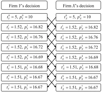
t + p+ ₌Z t p _{n = 0,1,2,…. (20)} It is also interesting to note that the concept of the si-mulated procedure itself matches the idea of a competitive view on firms in the market. In each iteration, one firm can access the other firm’s previous actions and determines its best move in price and lead time decision based on its own interests and constraints. In other words, the problem is a calculation of the succession of price and lead time de-cisions, where firms choose their optimum response given the price and lead time decisions of the competitors in the previous iteration. Next, we demonstrate the simulated procedure to solve for the equilibrium lead time and price in the example demonstrated in Section 2.3. The proce-dure starts from an initial estimate of the lead time and price as _{( ,}0 0_{, ,}0 0_{) (5,10,5,10)}

X X Y Y

t p t p = . The detailed steps of calculation are illustrated in Figure 1.

Firm Y’s decision Firm X’s decision 0 _{5, 10}0 Y Y t = p = 0 _{5, 10}0 X X t = p = 1 _{1.52, 16.82}1 Y Y t = p = 1 _{1.52, 16.82}1 X X t = p = 2 _{1.52, 16.76}2 X X t = p = 3 _{1.52, 16.72}3 X X t = p = 4 _{1.52, 16.69}4 X X t = p = 5 _{1.51, 16.68}5 X X t = p = 6 6 1.51, 16.67 X X t = p = 7 _{1.51, 16.67}7 X X t = p = 2 _{1.52, 16.76}2 Y Y t = p = 3 _{1.52, 16.72}3 Y Y t = p = 4 _{1.52, 16.69}4 Y Y t = p = 5 _{1.51, 16.68}5 Y Y t = p = 6 _{1.51, 16.67}6 Y Y t = p = 7 _{1.51, 16.67}7 Y Y t = p =

Figure 1: The calculation of the simulated procedure for the example

At iteration 7, the optimal move of the lead time and price is numerically identical to the solution of the pre-vious iteration. Neither firm X nor Y can improve its profit by a unilateral change in its solution of the lead time and price. The successive procedure returns that the equili-brium lead time and price are 1.51 and 16.67 respectively and the associated profit is 50.24. The simulated results are identical to the solution obtained in the combined KKT approach. It is also easy to verify that the optimal solution

Hong, Hsu, Wu, and Yeh of firm Y is

(

*_, *

)

(

_{1.51, 16.67}

)

Y Y

t p = given firm X’s solution,

(

*_, *

)

(

_{1.51, 16.67}

)

X X

t p = , and vice versa. The solution ob-tained in the KKT approach is indeed an equilibrium deci-sion whereby no one has incentive to deviate from its cur-rent solution.

4 CONCLUSIONS

This paper examines the competition in a duopoly semi-conductor foundry market consisting of two leading firms and other relatively small foundry plants, where pricing and lead time setting are two important decisions. Firms compete to provide goods or services to customers. We view each firm as a system, which is behaved as an M/M/1 queue. Each independent firm considers its own objective function and is subject to its own constraints. Meanwhile, the objective function of each firm not only depends on its own decision variables but also depends on the decision variables of the other competing firm. In this paper, each firm tries to maximize its own revenue by choosing its quotation of the lead time and price subject to the con-straint that the firm needs to satisfy the minimum required service level, which is defined as the probability of meet-ing the promised lead time quotation. Note that the quota-tion of the lead time and price of the other competing firm affects each firm’s revenue function in our model.

This paper proposes a method, the combined KKT ap-proach, to solve for the equilibrium decision of the lead time and the price for each competing firm in the market. In equilibrium, no firm would like to deviate from its cur-rent decision given others’ decision. The equilibrium solu-tion is obtained by simultaneously solving the sufficient KKT optimality conditions instead of necessary conditions. We show that the KKT optimality conditions of the duopo-ly model presented in this paper are sufficient so that the solution to the KKT conditions is an equilibrium decision. Finally, this paper utilizes a simulated procedure to ve-rify the equilibrium solution of the price and lead time ob-tained by the analytical KKT approach presented in this paper. This example numerically shows that both solutions obtained from the combined KKT approach and the itera-tive simulated method are identical. The model presented in this paper is a prototypical duopoly model and can be used as a tool to analyze a more complicated competing market and to draw managerial insights for such systems in future research.

ACKNOWLEDGMENTS

This research was supported in part by the National Science Council, Taiwan under Grants NSC96-2221-E-009-085 and NSC96-2221-E-009-035.

APPENDIX

Proof of Lemma 1. For notational simplicity, we rewrite the arrival rate λ as follows: i

0 1 1 1 2 2 2 1 2 0 1 2 3 4 ( , | , , , ) [ ( ) ( )] [ ( ) ( )] ' i i i j j M M i M i j i M i j i i j j t p t p t p m t t t t m p p p p u u t u p u t u p λ λ β α α β α α = − − + − − − + − = − − + + (21) where 0 0 1 1 1 1 2 2 1 1 1 2 2 2 3 2 1 1 4 2 2 2 1 2 3 4 ' , , , 0. M M u m t m p u m u m u m u m u u u u λ α β α β β β α β α β = + + = = = = >

By inserting (21) into (4) and rearranging it, we have

0 1 2

(u −u ti−u p ti)i ≤ln(1−s) (22) where

0 0' 3 j 4 j i

u =u +u t +u p − . μ

Proving that the profit function of firm i, π , is pseudo-_i concave is equivalent to showing that 'πi = − is pseudo-πi

convex. Since '

i

π is twice continuously differentiable, the gradient, ( ')∇πi , and Hessian matrix, ∇2( ')πi , of 'π can i

be computed as

[

]

' ' 2 1 ( ')T i i i i i i i i u p u p p t π π π ⎡∂ ∂ ⎤ λ ∇ =_{⎢ ⎥}= − + ∂ ∂ ⎣ ⎦ , and 2 2 2 2 1 2 2 2 1 2 ' ' 2 ( ') 0 ' ' i i i i i i i i i i i p t p u u u t p t π π π π π ⎡∂ ∂ ⎤ ⎢ _{∂ ∂ ∂} ⎥ ⎡ ⎤ ⎢ ⎥ ∇ =_{⎢ ⎥= ⎢ ⎥} ∂ ∂ ⎣ ⎦ ⎢ ⎥ ∂ ∂ ∂ ⎢ ⎥ ⎣ ⎦ . Rearranging (7), we have

(

)

(

)

(

)

(

)

(

)

(

)

(

)

(

)

2 2 1 2 2 1 2 1 _{1 2 1} 2 2 2 1 1 2 2 1 1 2 1 2 ( , ) 0 2 . i i i i i i i i i i i i i i i i i i u p u p u p u u M X u _{u p u p u p} u u p u u p u p u u p u p u p λ λ β β λ β λ β λ β λ β ⎡ _{− − −} ⎤ ⎡ ⎤ _{⎢ ⎥} =_{⎢ ⎥}+ _{⎢ ⎥} ⎣ ⎦ _⎣− − _⎦ ⎡ _{+ − − −} ⎤ ⎢ ⎥ = ⎢ ₋ ⎥ ⎣ ⎦ The determinant of ( , )M X β is 2

(

)

1 2 i i 1 u β λ − . We let p 1 2ϕ β = where ϕ= piλi and λi =u0'−u t1i−u p2 i+u t3 j+ 4 j

u p . It is obvious that ϕ is a lower bound of the profit function of firm i since the customer arrival rate is with the highest value for the variable with negative coefficients and the lowest value for the variable with positive coeffi-cients. As a result, the determinant of M X( , )β is positive for such β . In addition, the diagonal elements of

( , )

M X β are nonnegative. This gives the result that there exist a real numberβ , 0≤ < +∞β , such that M X( , )β is positive semi-definite. Following Definition 1, π is a i' pseudo-convex function.

Proof of Lemma 2. The feasible region C of constraints (4) – (6) can be represented as 0 1 2 , , ( , ) ( ) ln(1 ) i i i i i i i i i i i t t t p p p C t p u u t u p t s ⎧ _{≤ ≤ ≤ ≤} ⎫ ⎪ ⎪ = ⎨ ⎬ − − ≤ − ⎪ ⎪ ⎩ ⎭

We let zr1=( , )t p1 1 ∈C and zr2 =( ,t p2 2)∈C . Con-sider the point zr=( , )t p =αzr₁+ −(1 α) , 0zr₂ ≤ ≤α 1. Be-cause t1≤ and ti t2≤ , we have ti t=αt1+ (1−α)t2 ≤αti

(1 α)t_i t_i

+ − = . Since t₁≥t_i and t₂≥t_i , we have t=αt₁ 2

(1 α)t

+ − ≥αt_i+ −(1 α)t_i = . Therefore, t_i t_i ≤ ≤ . Si-t t_i milarly, p_i ≤ ≤p p_i . These show that (6) holds for

( , ) z= t p

r _.

Constraint (4) can be represented as (22). For zr₁ and 2 z r _{, we have} 0 1 1 2 1 ln(1 ) /1 u −u t −u p ≤ −s t (23) and 0 1 2 2 2 ln(1 ) / 2 u −u t −u p ≤ −s t . (24)

Considering zr=( , )t p , the left hand side of (22) can be rewritten as follows:

(

)

(

)

(

)

(

)

(

)

(

)

(

) (

)

0 1 2 0 1 1 2 2 1 2 1 2 0 1 1 2 1 0 1 2 2 2 1 2 (1 ) (1 ) (1 ) (1 ) (1 ) . u u t u p t u u t t u p p t t u u t u p u u t u p t t α α α α α α α α α α − − = − + − − + − + − =⎡_⎣ − − + − − − ⎤_⎦ + −

Because of (23) and (24), we have

(

)

(

)

0 1 2 1 2 1 2 ln(1 ) _{(1 )}ln(1 ) _{(1 )} u u t u p t s s _{t t} t t α α α α − − ⎛ − − ⎞ ≤_⎜ + − _⎟ + − ⎝ ⎠ 2 2 2 1 1 2 ln(1 s) (1 ) (1 )(t t ) . t t α α α α ⎛ ⎞ = − _⎜ + − + − + _⎟ ⎝ ⎠

Due to the Cauchy inequality (see Bartle 1976), we have

2 2 2 1 1 2 ln(1 s) (1 ) (1 )(t t ) t t α α α α ⎛ ⎞ − _⎜ + − + − + _⎟ ⎝ ⎠

(

)

(

)

2 2 2 ln(1 ) (1 ) 2 (1 ) ln(1 ) (1 ) ln(1 ). s s s α α α α α α ≤ − + − + − = − + − = − Therefore,

(

u0−u t u p t1 − 2

)

≤ln(1−s). (25)

Due to (25), zr=( , )t p also satisfies (4) and (5). In sum-mary, for zr₁=( , )t p_{1 1} ∈C and zr₂ =( ,t p_{2 2})∈C, we show that the point zr=( , )t p =αzr1+ −(1 α) , 0zr2 ≤ ≤α 1 satisfies constraints (4) – (6). It completes the proof.

REFERENCES

Bartle, R. G. 1976. The Elements of Real Analysis. 2nd

edi-tion. John Wiley & Sons, New York.

Bazaraa, M. S., H. D. Sherali, and C. M. Shetty. 1993. Nonlinear Programming Theory and Algorithm. John Wiley & Sons, New York.

Chang, S.-C. 2005. The TFT-LCD industry in Taiwan: competitive advantages and future developments. Technology in Society 27: 199-215.

Chen, H., and Y. W. Wan. 2003. Price competition of make-to-order firms. IIE Transactions 35: 817-832. Contreras, J., M. Klusch, and J. B. Krawczyk. 2004.

Nu-merical solutions to Nash-Cournot equilibria in coupled constraint electricity markets. IEEE Transac-tions on Power Systems 19(1): 195-206.

ElHafsi, M. 2000. An operational decision model for lead-time and price quotation in congested manufacturing

Hong, Hsu, Wu, and Yeh system. European Journal of Operational Research

126: 355-370.

Gibbons, R. 1992. Game Theory for Applied Economists. New Jersey: Princeton University Press.

Hatoum, K. W., and Y. L. Chang. 1997. Trade-off between quoted lead time and price. Production planning and control 8(2): 158-172.

Hobbs, B. F. 2001. Linear complementarity models of Nash-Cournot competition in bilateral and POOLCO power. IEEE Transactions on Power Systems 16(2): 194-202.

Hong, I-H., J. C. Ammons, and M. J. Realff. 2008. Centra-lized verse decentraCentra-lized decision-making for recycled material flows. Environmental Science & Technology, 42(4): 1172-1177.

Kalai, E., M. I. Kamien, and M. Rubinovitch. 1992. Op-timal service speeds in a competitive environment. Management Science 38(8): 1154-1163.

Krawczyk, J. B., and S. Uryasev. 2000. Relaxation algo-rithm to find Nash equilibria with economic applica-tions. Environmental Modeling and Assessment 5: 63-73.

Kleinrock, L. 1975. Queueing Systems. John Wiley & Sons, New York.

Lederer, P. J., and L. Li. 1997. Pricing, production, sche-duling, and delivery-time competitive. Operations Re-search 45(3): 407-420.

Li, L., and Y. S. Lee. 1994. Pricing and delivery-time per-formance in a competitive environment. Management Science 40(5): 633-646

Mereau, P., and J.G. Paquet. 1974. Second order condi-tions for pseudo-convex funccondi-tions. SIAM Journal on Applied Mathematics 27(1): 131-137.

Palaka, K., S. Erlebacher, and D. H. Kropp. 1998. Lead-time setting, capacity utilization, and pricing decisions under lead-time dependent demand. IIE Transactions 30: 151-163.

Ray, S., and E. M. Jewkes. 2004. Customer lead time man-agement when both demand and price are lead time sensitive. European Journal of Operational Research 153: 769-781.

So, K. C. 2000. Price and time competition for service de-livery. Manufacturing & Service Operations Man-agement 2(4): 392-409.

So, K. C., and J. S. Song. 1998. Price, delivery time guar-antees and capacity selection. European Journal of Operational Research 111: 28-49.

Stalk, G. Jr. 1988. Time-the next source of competitive ad-vantage. Harvard Business Review July-August 41-51. Stalk, G. Jr., and T. M. Hout. 1990. Competing Against

Time. The Free Press, New York.

The Register 2003. TSMC foundry market share dips.

Available via <

http://www.theregister.co.uk/2003/08

/22/tsmc_foundry_market_share_dips/>

[accessed April 14, 2008]. AUTHOR BIOGRAPHIES

I-HSUAN HONG is an Assistant Professor in the Depart-ment of Industrial Engineering and ManageDepart-ment at Na-tional Chiao Tung University in Taiwan. He received his MS degree from National Taiwan University and his PhD in Industrial and Systems Engineering from Georgia Insti-tute of Technology, Atlanta, U.S.A. His research areas in-clude reverse logistics systems, competition models in multi-echelon supply chains, application and methodolo-gies for game theory.

HSI-MEI HSU received the MBA degree from Osaka University, Osaka, Japan, in 1975, and the PhD degree in industrial engineering from National Tsing-Hua University, Taiwan, in 1991. She is a Professor in the Department of Industrial Engineering and Management, National Chiao Tung University, Taiwan. Her research interests include production management, supply chain management, and multiple criteria decision making.

YI-MU WU received his MS degree from National Chiao Tung University in Taiwan and currently works in the in-dustry.

CHUN-SHAO YEH is currently a Master student in the Department of Industrial Engineering and Management at National Chiao Tung University in Taiwan.