國際能源價格與台灣總體經濟變數之關聯性分析

行政院國家科學委員會專題研究計畫 成果報告

國際能源價格與台灣總體經濟變數之關聯性分析

研究成果報告(精簡版)

計 畫 類 別 ： 個別型 計 畫 編 號 ： NSC 98-2410-H-009-055- 執 行 期 間 ： 98 年 08 月 01 日至 99 年 09 月 30 日 執 行 單 位 ： 國立交通大學經營管理研究所 計 畫 主 持 人 ： 胡均立 計畫參與人員： 碩士班研究生-兼任助理人員：蔡芳紜 博士班研究生-兼任助理人員：林政勳 博士班研究生-兼任助理人員：葉芳瑜 博士班研究生-兼任助理人員：張子溥 報 告 附 件 ： 出席國際會議研究心得報告及發表論文 處 理 方 式 ： 本計畫可公開查詢

中 華 民 國 99 年 09 月 28 日

國際能源價格與台灣總體經濟變數之關聯性分析

A Linkage Analysis of International Energy Prices and

Macroeconomic Variables in Taiwan

計畫編號：NSC

98-2410-H-009-055

計畫報告

執行期限：民國 98 年 8 月 1 日至 99 年 9 月 30 日（申請延長執行期

限獲准）

主持人：胡均立 國立交通大學經營管理研究所

兼任研究助理：林政勳、葉芳瑜、張子溥、蔡芳紜

電子信箱(E-mail)位址：

jinlihu@mail.nctu.edu.tw

Table of Contents

Abstract (in Chinese) 3

Abstract (in English) 4

1 Introduction 5

1.1 Research Background 5

1.2 Research Motivation and Purpose 6

2 Literature Review 8

3 Methodology 12

3.1 Unit Root Tests 12

3.1.1 Augmented Dickey Fuller (ADF) Test 12

3.1.2 The Kwiatkowski, Phillips, Schmidt, and Shin (KPSS) Test 13

3.2 Cointegration Analysis 14

3.3 Multivariate Threshold Error Correction (MVTEC) Model 17

3.4 Impulse Response Analysis 19

3.5 Variance Decomposition 23

4 Empirical Results 25

4.1 Data Description 25

4.2 One-regime VAR analysis 26

4.2.1 Results of Tests for Unit Roots and Cointegration 26

4.2.2 Results of the Variance Decomposition 29

4.2.3 Results of the Impulse Response Analysis 30

4.3 Two-regime VAR analysis 33

4.3.1 Estimating the Threshold Levels and the Delay of

Threshold Variables 33

4.3.2 Results of the Variance Decomposition in the

MVTEC Model 34

4.3.3 Results of the Impulse Response Analysis in the

MVTEC Model 37

4.3.4 Results of the Parameter Stability Tests 41

5 Preliminary Conclusions and Policy Implications 44

國際能源價格與台灣總體經濟變數之關聯性分析

中文摘要 台灣為一能源有限且能源進口依存度高達 99.32 %的海島型經濟體。隨著國 際能源價格不斷攀高，國際能源價格的變動對台灣總體經濟活動之影響將值得深 入研究。本論文利用線性與非對稱的架構去評估國際能源價格(原油、煤炭、天 然氣)與台灣總體經濟變數(工業生產指數、股價、利率、失業率、進口值與出口 值等)之間的關係。利用 Tsay (1998) 所提出的多變量門檻模型結合非對稱動態調 整過程加以分析，以能源價格變動當作一個門檻變數區分為能源價格上漲與下跌 狀態，檢視在不同狀態下國際能源價格衝擊對台灣總體經濟活動的影響，進一步 利用衝擊反應分析與變異數分解去評估能源價格波動對台灣總體經濟之衝擊。研 究結果顯示：(1)油價的最適門檻值 2.48%，其次為天然氣價格門檻值 0.87%，最 小為煤價門檻值 0.22%；(2)當油價大於門檻值時，油價對於工業生產值上的解釋 能力更甚於利率；(3)當天然氣價格小於門檻值時，天然氣價格分別在股價與失 業率上面都具有較大的解釋能力；(4)煤價衝擊與天然氣價格衝擊均對於台灣總 體經濟活動而言具有延遲的負面影響。 關鍵詞：能源價格衝擊、總體經濟活動、多變量門檻誤差修正模型、衝擊反應分 析、變異數分解

A Linkage Analysis of International Energy Prices and

Macroeconomic Variables in Taiwan

Abstract

This paper applies a linear and asymmetric model to estimate the effects of international energy price shocks (including oil, coal, and natural gas prices) on Taiwan’s macroeconomic activity (such as industrial production, stock price, interest rate, unemployment rate, imports and exports). We apply a multivariate threshold error correction model by Tsay (1998) to analyze the empirical data. By separating energy price changes into the decrease and increase, the energy price change as a threshold variable can analyze different impacts of energy price changes and their shock on industrial production. The variance decomposition and the impulse response functions are also employed to analyze the short-run dynamics of the variables. The preliminary findings are: (1) The optimal threshold levels are that the highest level is oil price at 2.48%, the next highest is natural gas price at 0.87%, and the lowest level is coal price at 0.22%. (2) If the change is above the threshold levels, then a change in oil price explains industrial production better than the interest rate. (3) If the change is below the threshold levels, then it appears that the change in natural gas price better explains stock prices and the unemployment rate than the interest rate. (4) Both oil price shock and natural gas shock have a delayed negative impact on macroeconomic activities.

Keywords: Energy Price Shocks; Macroeconomic Activity; Multivariate Threshold Error Correction (MVTEC) Model; Impulse Response Analysis; Variance Decomposition

1 Introduction

1.1 Research Background

Energy price shocks are generally acknowledged to have important effects on both the economic activity and macroeconomic policy of industrial countries. Huge and sudden rises in energy prices increase inflation and reduce real money balances with negative effects on consumption and output. Since the 1970s, oil price in the world market has experienced fluctuations including sharp rises during the first and second oil crises. During the periods of 1973-1974 and 1978-1979, when the Organization of Petroleum Exporting Countries (OECD) first imposed an oil embargo and the Iranian revolution disrupted oil supplies, the prices of a barrel of oil increased from $3.4 to $30. In 1990, prices rapidly rose from $16 to $26 after the Gulf War. Recently, the WTI oil future prices averaged $76 per barrel in October 2009 on the New York Mercantile Exchange (NYMEX).

Higher prices of oil driving demand for other energy have made natural gas and coal more competitive. Because price-setting is based on production costs and applications for rate increases move slowly through the bureaucratic process, natural gas volatility is quite small. On average, natural gas price variability is 3%-4%. The monthly average coal price reached a record high of $208.55 per mcf in 2008. Coal prices saw severe fluctuations during 2003 to 2009.

Domestic energy price-setting is relatively affected by projected world oil prices in the past several years. Jiménez-Rodríguez and Sánchez (2005) report that oil price increases have a direct impact on economy activity for oil-importing countries. Indeed, rising oil prices are interpreted as an indicator of an increase in scarcity and that means oil will be less available on the domestic market. This phenomenon is expected to keep the domestic energy price at high levels over the near term.

In sharp contrast to the volume of studies examining the link between oil price shocks and macroeconomic variables, there is currently not much existing literature on quantitative analyses of coal-price or gas-price shocks. There are also few analyses on the relationship between oil price shocks and financial markets such as the stock market. Market participants want a framework that identifies how energy price changes affect the stock market and labor market.

1.2 Research Motivation and Purpose

As energy prices play a critical role in influencing economic growth and economic activities, this phenomenon excites the research interest of this dissertation to address a linkage analysis of international energy prices and macroeconomic variables in Taiwan with linear and non-linear frameworks. Our research is motivated by the following reasons.

First, most studies (e.g., Burbidge and Harrison, 1984; Gisser and Goodwin, 1986; Mork, 1989; Hooker, 1996; Hamilton, 1996; Bernanke et al., 1997; Hamilton, 2003; Hamilton and Herrera, 2004) show that oil price shocks have a significantly negative impact on industrial production. However, little is known about the relationship between other energy prices and economy activities. For this reason, researchers may refocus their attention on the issue of natural gas price and coal price and their impact on economic activities.

Second, some of the related research (e.g., Mork, 1989; Mork et al., 1994; Sadorsky, 1999; Papapetrou, 2001; Hu and Lin, 2008) already consider the asymmetrical relation in terms of the impact of an oil price change or its volatility on industrial production and stock returns. However, these studies arbitrarily use zero as a cutoff point and distinguish oil price changes into up (increase) and down

(decrease). This shows that the traditional approaches using predetermined value(s) as a demarcation point are rather unreasonable. They neglect the asymmetrical relation to accurately gauge varying degrees of impacts of energy price change (or volatility) on macroeconomy. To solve the neglected phenomenon, we implement rigorous econometric methods to refine the true relation.

Third, early studies about the macroeconomic consequences of energy price shocks focus on developed economies. Recent studies examine other research samples such as European countries (e.g., Mork et al, 1994; Papapetrou, 2001; Cunado and Pérez de Gracia, 2003; Jiménez-Rodríguez, 2008; Bjørnland, 2009) and Asian countries (e.g., Chang and Wong, 2003; Cunado and Pérez de Gracia, 2005; Huang et al., 2005). However, few studies investigate the relationship between energy price and macroeconomy for Taiwan. In contrast to these studies, this dissertation assesses the dynamic effect of energy price shocks on the macroeconomy in Taiwan.

Based on the aforementioned argument, the purposes of this dissertation contain two parts: The first purpose is to examine the effects of energy price shocks (including crude oil, natural gas and coal) on Taiwan’s industrial production from a linear perspective. Energy prices do not affect industrial production in isolation, but through the perceived effect on the macroeconomy. Therefore, we further analyze the dynamic relationship between energy price shocks and major macroeconomic variables (including stock price, interest rate, unemployment rate, exports and imports) by applying a vector error correction (VECM) model. Next, the variance decomposition (VDC) and the impulse response functions (IRF) are employed to capture the effects of energy price shocks on the macroeconomy. The results find how each variable responds to shocks by other variables of the system and explore the response of a variable to a shock immediately or with various lags.

The second purpose focuses on the impacts of an energy price change and the shock on the macroeconomy from an asymmetric perspective. According to Sadorsky (1999), the energy price adjustment may not immediately impact macroeconomic variables. An economic threshold for an energy price impact is the amount of price increase beyond which an economic impact on industrial production and stock prices is palpable. Huang et al. (2005) propose that a change in oil price explains the macroeconomic variables better than the shock caused by the oil price if an oil price change exceeds the threshold levels. Therefore, we apply the multivariate threshold error correction model by Tsay (1998) to analyze the relevant data. By separating energy price changes into decrease (down) and increase (up), the energy price changes as the threshold variable can analyze different impacts of energy price changes on industrial production. In particular, we assess the impact of energy price fluctuations on the Taiwan economy. The impulse response and the variance decomposition analysis now follow.

2 Literature Review

Since the 1970s many studies have examined the relationship between energy prices and the macroeconomy especially for oil price shocks. However, there is an inconsistent conclusion in the literature with different estimation procedures and data. According to the different energy prices used by researchers, previous studies can be divided into three streams of research: the impact of oil price on GDP, the impact of oil price on other macroeconomic variables, and the natural gas and coal price effect.

Hamilton (1983) using Granger causality examines the impact of oil price shocks on the United States economy, indicating that oil price increases partly account for every United States recession. Many researchers extend and reinforce Hamilton’s basic findings using different estimation procedures on new data (e.g., Burbidge and

Harrison, 1984; Gisser and Goodwin, 1986; Mork, 1989; Hooker, 1996; Hamilton, 1996; Bernanke et al., 1997; Hamilton, 2003; Hamilton and Herrera, 2004). These studies conclude that there is a significant negative correlation between increases in oil prices and the subsequent recessions in the United States, but that oil price changes have different impacts on economies over time.

By separating oil price changes into negative and positive, Mork (1989) finds that there is an asymmetrical relationship between oil price and real output. When the oil price is increasing, the increase in the cost of production and the decrease in the cost of resource allocation often offset each other. Mory (1993) follows Mork’s (1989) measures and presents that positive oil price shocks Granger-cause the macroeconomic variables. Mork et al. (1994) again confirm that oil price shock induced inflation reduces real balances for seven industrialized countries. Lee et al. (1995) find that an oil shock in a price stable environment is more likely to have greater effects on GDP growth than those occurring in a price volatile environment. Jiménez-Rodríguez and Sánchez (2005) find that oil price increase has a larger impact on GDP growth than oil price declines.

In addition to exploring the relationship between oil price shocks and GDP, some economists have emphasized the relationship between oil price shocks and other macroeconomic variables. The first part is related to the macroeconomic level. Several models (e.g., Rasche and Tatom, 1981; Bruno and Sachs, 1982, Hamilton, 1983) and diverse episodes for oil price shocks (e.g., Davis, 1986; Carruth et al., 1998; Ferderer, 1996) present that an oil shock is one of the important influences on the macroeconomy. The directions for the causal relationship between oil price and macroeconomy can be concluded in four parts. First, oil price changes significantly impact economic activity (e.g., Papapetrou, 2001; Ewing et al., 2006; Jiménez-Rodrí guez, 2008; Farzanegan and Markwardt, 2009). Second, there is an asymmetric

correlation between oil price and the macroeconomy (e.g., Loungani, 1986; Mork, 1989; Lee et al., 1995; Hamilton, 2003; Cunado and Pérez de Gracia, 2003; Cunado and Pérez de Gracia, 2005; Jiménez-Rodríguez, 2009). Third, some researchers show effects of oil price shocks at a disaggregate level.

The second part is related to stock markets. Kaneko and Lee (1995) find that Japanese stock prices are affected by oil price shocks. Jones and Kaul (1996) further investigate the reaction of stock prices to oil price shocks and what may justify these movements. By using a cash-flow/dividend valuation model (i.e., Campbell, 1991), they find that oil prices can predict stock returns and output on their own. Sadorsky (1999) discovers that oil price movements can explain more of the forecast error variance of stock returns than can interest rates. Some studies (e.g., Lo and MacKinlay, 1990; Kaul and Seyhum, 1990; Sadorsky, 2003; Park and Ratti, 2008) propose that an increased volatility of oil prices significantly depresses real stock returns. Bjørnland (2009) indicates that following a 10% increase in oil prices, Norway’s stock returns increase by 2.5%. Apergis and Miller (2009) also find that different oil market structural shocks play a significant role in explaining the adjustments in stock returns.

The third part involves the labor market. A clear negative relationship between oil prices and employment is reported by Rasche and Tatom (1981), Hamilton (1983), Keane and Prasad (1996), Uri (1996), Raymond and Rich (1997), among others. Keane and Prasad (1996) further indicate that oil price increases reduce employment in the short run, but tend to increase total employment in the long run. An oil price decrease depresses demand for some sectors, and unemployed labor is not immediately shifted elsewhere (Hamilton, 2003). However, oil price changes impact unemployment when the changes in oil prices persist for a long time as adjustments in employment (Keane and Prasad, 1996). Carruth et al. (1998) present an

asymmetrical relationship among unemployment, real interest rates, and oil prices, meaning that oil price increases cause employment growth to decline more than oil price decreases cause employment growth to increase. Davis and Haltiwanger (2001) find an oil price shock can explain 25% of the cyclical variability in employment growth from 1972 to 1988.

Most studies show the effect of oil price shocks, but rarely consider the effect of natural gas or coal price shocks. Coal and natural gas are the two main alternative sources of energy. There are three effects of changing natural gas price controls: on regional economic activity (e.g., Leone, 1982), on inflation (e.g., Ott and Tatom, 1982), and on the distribution of income between households and suppliers (e.g., Stockfisch, 1982). Hickman et al. (1987) examine the correlation between natural gas price and industrial production. They indicate that a 10% increase in natural gas price affects the same effect on real GDP growth. Jin et al. (2009) find that energy prices have significant negative effects on real economic growth and oil price shocks are greater than other resources. Lutz and Meyer (2009) observe that a stabilizing effect via international trade and domestic structural change on the GDP of oil importing countries with a permanent oil price increase occurs.

Researchers have begun to analyze the causality relationship between coal consumption and economic growth in recent years. Yang (2000) shows a causality relationship between coal consumption and economic growth in Taiwan. Yoo (2006) finds that bidirectional causality running from GDP to coal consumption exists in South Korea. Both Li et al. (2008) and Li et al. (2009) cover that there is unidirectional causality between coal consumption and GDP in China and Japan. However, there are few studies specifically addressing coal price with economic growth.

3 Methodology

3.1 Unit Root Tests

3.1.1 Augmented Dickey Fuller (ADF) Test

Dickey and Fuller (1979) consider a autoregressive process AR(1) model 1 1

t t t

y a y_  , where the disturbances, _t , are assumed to be white noise, conditional on past yt, and the first observation, y1, is assumed to be fixed. By subtracting y_t1 from both sides of the equation, we can rewrite the model as follows:

1

t t t

y y_ 

   , where   a1 1. The unit root test is equivalent to testing 0, that is, that there exists a unit root. The standard t-statistic for ˆ can be used to test 0, but with the Dickey-Fuller critical values.

However, simple unit root test described above is valid only if the series is an AR(1) process. If the series is correlated at higher order lags, the assumption of

white noise disturbances is violated. Dickey and Fuller (1981) make a parametric correction for higher order correlation by assuming that the

 

y_t follows an AR(p) process and extending model as follows:

0 1 1 2 2 1 1

t t t p t p p t p t

y a a y_ a y_  a _ y_{ } a y_  (1) By adding and subtracting a y_{p t p 1} from both sides of the equation then the differenced form is:

0 1 1 2 2 2 2 ( 1 ) 1 1

t t t p t p p p t p p t p t

y a a y_ a y_  a _ y_{ }  a _ a y_{ }  a y_{ }  (2) Next, add and subtract (a_p1a_p)y_{t p 2} to obtain:

0 1 1 2 2 ( 1 ) 2 1

t t t p p t p p t p t

y a a y_ a y_   a _ a y_{ }  a y_{ }  (3) Continuing in this fashion, we get:

0 1 1 2 p t t i t i t i y a y_  y_{ }      



  , (4)

where 2 1 p i i a       _{ } 



 and p i j j i a   



In Eq. (4), the coefficient of interest is . If  0, the equation is entirely in first differences and so has a unit root. Three ADF test actually consider three different regression equations that can be used to test for the presence of a unit root:

1 1 2 p t t i t i t i y y_  y_{ }     



  (5) 0 1 1 2 p t t i t i t i y a y_  y_{ }      



  (6) 0 1 2 1 2 p t t i t i t i y a y_ a t  y_{ }       



  . (7) The differences between the three regressions concerns the presence of the deterministic elements a0 and a t2 . Without an intercept and time trend belongs in Eq. (5); with only the intercept belongs in Eq. (6); and with both an intercept and trend belongs in Eq. (7). If the coefficients of a difference equation sum to one, at least one characteristic root is unity. If  a_i 1 and  0, the system has a unit root.

3.1.2 The Kwiatkowski, Phillips, Schmidt, and Shin (KPSS) Test

Kwiatkowski et al. (1992) propose a test of the null hypothesis that an observable series is stationary around a deterministic trend. The series is expressed as the sum of deterministic trend, random walk, and stationary error, and the test is the LM test of the hypothesis that the random walk has zero variance. The KPSS statistic is based on the residuals from the OLS regression of y_t on the exogenous variablesx_t:

t t t

y x 

The Lagrange Multiplier (LM) statistic can be defined as: 2 2 1 ˆ / T t t LM S _  



,

where S_t is a cumulative residual function (i.e., 1 ˆ , 1, 2, , t t i i S  i T  



 ). We

point out that the estimator of  used in this calculation differs from the estimators for  used by detrended GLS since it is based on a regression involving the original data and not on the quasi-differenced data. Finite sample size and power are considered in a Monte Carlo experiment.

Prior to performing the Johansen co-integration method, we need to determine the appropriate number of lag length of the VAR model. The Bayesian information criterion (BIC) (Schwarz, 1978) is employed. The test criteria to determine appropriate lag lengths and seasonality are the multivariate generalizations of the BIC. The BIC criterion is a purely statistical technique and allows data themselves to select optimal lags. Given any two estimated models, the model with the lower value of BIC is the one to be preferred. The selection of lag order of yt i can be used by the Bayesian information criterion (BIC):

BIC=-2*ln(L)+k*ln(n) (8)

where n is the number of observations, k is the number of free parameters to be estimated and L is the maximized value of the likelihood function for the estimated model. The BIC penalizes free parameters more strongly than does the Akaike information criterion (AIC) (Akaike, 1969).

3.2 Cointegration Analysis

The Johansen co-integration method is provided by Johansen (1988) and Johansen and Juselius (1990). This procedure applying maximum likelihood estimators circumvent the low-power of using Granger two-step estimators and can estimate and test for the presence of multiple cointegrating vectors. Moreover, this test allows the researcher to test restricted versions of the cointegrating vectors and

speed of adjustment parameters.

Let y_t denotes the (n1) vector(y y_{1 ,t 2 ,t}..._,y_nt). The maintained hypothesis is that y_t follows a VAR(P) in levels and all of the elements for y_t are I(1) process.

1 +A2 + +Ap + ,t 1, 2, , A  t T   t t-1 t-2 t-p y y y y (9) where . . . (0, ) i i d t N    .

Eq. (10) can be put in a more usable form by subtracting yt1 from each side to obtain:

1 2

(A I) +A + +Ap + ,t t 1, 2, ,T

 yt  yt-1 yt-2 yt-p  (10)

Now add and subtract (A1I)yt-2 to obtain:

1 2 1

(A I) +(A A I) + +A_p + ,_t t 1, 2, ,T

 y_t  y_t-1   y_t-2 y_t-p  (11) Continuing in this fashion, we obtain:

1 1 p t i       yt



yt-i yt-p (12) where 1 p i i I A      _  _ 



 1 i i j j I A      _  _ 





Suppose we obtained the matrix  and order the n characteristic roots such that ₁ ₂  ... _n. If the variables in y_t are not cointegrated, the rank of  is zero and all these characteristic roots will equal zero. Similarly, since ln(1)0, each of the expressions ln(1_i) will equal zero if the variables are not cointegrated.

Suppose that each individual variable y_it is I(1) and linear combinations of y_t are stationary. That implies  can be shown as

where β is the matrix of cointegrating parameters, and  is the matrix of the speed of adjustment parameters. The number of cointegrating relations relies on the rank of , and the rank of  is:

(1) rank( ) n,  is full rank means that all components of y_t is a stationary process.

(2) rank( ) 0 ,  is null matrix meaning that there is no cointegration relationships.

(3) 0rank( )  r n, the variables for y_t are cointegrated and the number of cointegrating vectors is r.

The test for the number of characteristic roots that are insignificantly different from unity can by conducted using the following two test statistics:

(1) Trace test: 1 ˆ ( ) ln(1 ) n trace i i r r T      



 , 0: rank( ) H  r, 1: rank( ) H  r

where ˆ_i is the estimated values of the characteristic roots (also called eigenvalues) obtained from the estimated  matrix, r is the cointegrating vector, and T is the number of usable observations. The statistic tests the null hypothesis that the number of distinct cointegrating vectors is less than or equal to r against a general alternative. If there is no cointegrating vector, it should be clear that _trace equals zero when allˆ_i 0. The further the estimated characteristic roots are from zero, the more negative is ln(1ˆ_i) and the larger the _trace statistic.

(2) Maximum eigenvalues test: max( ,r r 1) Tln(1 ˆr 1)

0

H : there are r cointegrating vectors 1

H : there are r1 cointegrating vectors

The statistic tests the null that the number of cointegrating vectors is r against the alternative of r1 cointegrating vectors. If the estimated value of the characteristic root is close to zero, max will be small. The critical values of the

trace

 and _max statistics follows a chi-square distribution in general.

3.3 Multivariate Threshold Error Correction (MVTEC) Model

At the beginning, we consider the univariate TAR model which is also referred to as SETAR (self-exciting TAR). The SETAR(1) can be formed as:

0,1 1,1 1 1 0,2 1,2 1 1

y_t (  y )(1_t I z[ _t c]) (   y ) [_t I z_t  c] _t (13) where _t is a white noise process, z_t1 y_t1, and c represents the threshold value.

( )

I  is an index function, which equals to one if the relation in the brackets holds, and equals to zero otherwise. Eq. (13) can be treated as a multivariate threshold VAR(1). Consider a k-dimensional time series yt (y1t, ,ykt)and assume there is a cointegration relationship among these variables, then y_t follows a multivariate threshold error correction model (MVTEC) with threshold variable zt and delay d and can be expressed as:

1 1 1 ,1 1 2 2 1 ,2 1 ( )(1 [ ]) ( ) [ ] (14) p t i t d i p t i t d t i I z c I z c                         





t t-i t-i y y y

where 1 and 2 are the constant vectors below and above the threshold value, respectively. p and d are the lag length of y_t and delay order of z_t, respectively. Both p and d are nonnegative integers. t1 is an error correction term. The threshold variable is assumed to be stationary and have a continuous distribution. Model (14) has two regimes and is a piecewise linear model in the threshold space

t d

z_ .

Given observations



y_t, z_t



, wheret 1, ,n, we have to detect the threshold nonlinearity ofy_t. Assuming p and d are known, the Eq. (14) can be re-written as:

Xt t, t h 1, ,n

t      

y (15) where hmax( , )p d , X_t (1, y ,_t1 y_{tt p} ,_t1) is a (pk1)-dimensional regressor, and Φ denotes the parameter matrix. If the null hypothesis holds, then the least squares estimates of (15) are useful. On the other hand, the estimates are biased under the alternative hypothesis. Eq. (15) remains informative under the alternative hypothesis when rearranging the ordering of the setup. For Eq. (15), the threshold variable z_{t d} assumes values in S 



z_{h 1 d}, z_{n d}



. Consider the order statistics of S and denote the ith smallest element of S by z . Then the arranged regression _{( )i} based on the increasing order of the threshold variable z_{t d} is

( ) ( )

Xt id t id, i 1, ,n h

t(i)+d      

y Φ , (16) where ( )t i is the time index of z . Tsay (1998) use the recursive least squares _{( )i} method to estimate (16). If yt is linear, then the recursive least squares estimator of the arranged regression (16) is consistent, so the predictive residuals approach white noise. Consequently, predictive residuals are uncorrelated with the regressor

( ) X_{t id}.

Let Φm be the least squares estimate of Φ of Eq. (16) with i1, ,m; i.e., the

estimate of the arranged regression using data points associated with the m smallest values of z_{t d} . Tsay (1998) suggests a range of m (between 3 n and 5 n ). Different values of m can be used to investigate the sensitivity of the modeling results with respect to the choice. It should be noted that the ordered autoregressions are

sorted by the variablezt d , which is the regime indicator in the MVTEC model. Let ( 1) ˆ ( 1) ˆe_{t m d} y_t(m+1)+d-Φ _μX_{t m d} (17) and 1/ 2 ( 1) ( 1) ( 1) ( 1) ˆ_{t m d} ˆe_{t m d} / 1 X_{t m d}V X_{m t m d}  _{ }  _{ } _   _{   } _ , (18) where V =_m __im_1X_{t i( )d}X_{t i( )d}_1 is the predictive residual and the standardized predictive residual of regression (16). These quantities can be efficiently obtained by the recursive least squares algorithm. Next, consider the regression

( ) ( ) ( ) 0

ˆt l d Xt l d wt l d, l m 1, ,n h

 _   _    _    , (19) where m0 denotes the starting point of the recursive least squares estimation. The problem of interest is then to test the hypothesis H₀: 0 versus the alternative

1: 0

H   in regression (19). The C d statistic is therefore defined as: ( )



1



( ) ( 1) ln S_o ln S

C d  n  p m kp   , (20) where the delay d implies the test depends on the threshold variable z_{t d} , and

0 ( ) ( ) 1 0 1 ˆ ˆ S n h o t l d t l d l m n h m           



and 0 1 ( ) ( ) 1 0 1 ˆ ˆ S w w n h t l d t l d l m n h m         



,

where ˆw_t is the least squares residual of regression (19). Under null hypothesis the

yt is linear and some regularity conditions, C(d) is asymptotically a chi-squared random variable with k pk( 1) degree of freedom.

3.4 Impulse Response Analysis

12 13 17 1 10 11 12 13 17 1 1 1 21 23 27 2 20 21 22 23 27 2 1 2 71 72 73 7 70 71 72 73 77 7 1 7 1 1 1 t t t t t t t t t b b b y b y b b b y b y b b b y b y                                                 _{ }    _                                     

We can write the system in the compact form:

   t 0 1 t-1 t By Γ Γ y ε where 12 13 17 21 23 27 71 72 73 1 1 1 b b b b b b b b b     _        _    B , 1 2 7 t t t y y y              t y , 10 20 70 b b b              0 Γ , 11 12 13 17 21 22 23 27 71 72 73 77                 _        _    1 Γ .

Premultiplication by B-1 can obtain the vector autoregressive (VAR) model in standard form: 0 1 A A et  -1  -1  -1    t 0 1 t-1 t t-1 y B Γ B Γ y B ε y (21) where A₀ B Γ , -1 ₀ A1 -1 1

B Γ and etB ε . For notional purposes, we can -1 t define aio as element i of the vector A0, aij as the element in row i and column j of the

matrix A1, and eit as the element i of the vector et. Using this new notation, we can

rewrite (21) in the equivalent form:

1 10 11 1 1 12 2 1 17 7 1 1 2 20 21 1 1 22 2 1 27 7 1 2 7 70 71 1 1 12 2 1 17 7 1 7 t t t t t t t t t t t t t t t y a a y a y a y e y a a y a y a y e y a a y a y a y e                            (22) or

1 10 11 12 17 1 1 1 2 20 21 22 27 2 1 2 7 70 71 72 77 7 1 7 t t t t t t t t t y a a a a y e y a a a a y e y a a a a y e                          _  _     _                               (23) In model (21), the stability condition is that A0 be less than unity in absolute

value. Using the backward method to iterate model (21), we can obtain: 0 1 0 1 2 1 0 1 1 ( ) ( ) A A A A I A A A A           t t-2 t-1 t t-2 t-1 t y y ε ε y ε ε where I  7 7 identity matrix.

Assuming the stability condition is met, so that we can write the particular solution for yt as:

1 0 μ i i A    



t t-i y e . (24)

It is important to note that the error terms (i.e., e1t, e2t,…, e7t) are components of the seven shocks e1t , e2t ,…, e7t . Since 

-1 t t e B ε , we can compute

 

e1t ,

 

e2t ,…,

 

e7t as:

 

1 11 12 17 1 2 21 22 27 2 7 71 72 77 7 det t t t t t t e c c c e c c c b e c c c                 _                       (25)

Using model (24), model (23) can be re-written as:

1 1 11 12 17 1 2 2 21 22 27 2 0 7 7 71 72 77 7 i t t i t t i i t t i y y a a a e y y a a a e y y a a a e                       _ _                            



(26)

sequences. However, it is insightful to rewrite (26) in terms of the

 

_1t ,

 

_2t ,…,

 

_7t sequences. Equations (25) and (26) can be combined to form:

 

1 1 11 12 17 11 12 17 1 2 2 21 22 27 21 22 27 2 0 7 7 71 72 77 71 72 77 7 det i t t t t t t i t t t y y a a a c c c e y y a a a c c c e b y y a a a c c c e                         _ _                                    



Since the notation gets unwieldy, we can simplify by defining the 7×7 matrix i with elements_jk( )i :

 

11 12 17 21 22 27 1 71 72 77 det i i c c c c c c A b c c c            _{  }    

Hence, the moving average representation of (26) can be written in terms of the

 

1 y t  ,

 

2 y t  ,…,

 

7 y t  sequences: 1 2 7 1 1 11 12 17 2 2 21 22 27 0 7 7 71 72 77 ε ( ) ( ) ( ) ε ( ) ( ) ( ) ( ) ( ) ( ) ε y t i t y t i t i t y t i y y i i i y y i i i y y i i i                                  _ _                          _{  }



or more compactly, 0 μ _i i     



t t-i y ε . (27) The coefficients of i can be used to generate the effects of  y t₁, y t₂ , ,y t₇  shocks on the entire time paths of the

 

y_1t ,

 

y_2t ,…,

 

y_7t sequences. It should be clear that forty-nine elements _jk(0) are impact multiplier. For instance, the coefficient ₁₂(0) is the instantaneous impact of a one-unit change in εzt on yt. In

the same way, the elements11(1),12(1),…, 17(1) are the one period responses of unit changes in 1 1, 2 1, , 7 1 y t y t y t  _  _  _  

  on y1t , respectively. Updating by one period indicates that₁₁(1),₁₂(1),…,₁₇(1)also represent the effects of unit changes in

1, 2 , , 7

y t y t y t

  

 

  on y_{1 1t} .

The accumulated effects of unit impulses in

1, 2, , 7

y t y t y t

  

 

  can be obtained

by the appropriate addition of the coefficients of the impulse response functions. Note that after n periods, the effect of

2

y t

 on the value of y_{1t n} is₁₂( )n . Thus, the cumulated sum of the effects of

2

y t

 on the

 

y_1t sequence is: 12 0 ( ) n i i  



Letting n approach infinity yields the long-run multiplier. Since the

 

y_1t ,

 

y_2t ,…,

 

y7t sequences are assumed to be stationary, it must be the case that for all j and k, 2 0 ( ) jk i i   



is finite. The sets of coefficients11( )i ,12( )i , …,77( )i are called the impulse response functions. We can plot the impulse response functions (i.e., plotting the coefficients of jk( )i against i) is a practical manner to visually present the behavior of the

 

y_1t ,

 

y_2t ,…,

 

y_7t series in response to the various shocks.

3.5 Variance Decomposition

If we use the equation (27) to conditionally forecastyt1, the one-step ahead forecast error is₀ε_t1. In general,

0 μ i i     



t+n t+n-i y ε ,

1 0 n t i i E     



t+n t+n t+n-i y y ε

Forecasting solely on the {x1t} sequence, the n-step ahead forecast error is:

11 11 11 12 12 12 13 13 13 1 1 1 (0) (1) ( 1) (0) (1) ( 1) (0) (1) ( 1) (0) (1) ( 1) t n n n E n n n n                                   1 1 1 2 2 2 3 3 3 n n n 1t+n 1t+n y t+n y t+n-1 y t+1 y t+n y t+n-1 y t+1 y t+n y t+n-1 y t+1 y t+n y t+n-1 y t+1 y y ε ε ε ε ε ε ε ε ε ε ε ε

Denote the variance of the n-step ahead forecast error variance of y_{1t n}

as 1 2 ( ) y n  : 1 1 2 3 2 2 2 2 2 2 2 2 2 11 11 11 12 12 12 2 2 2 2 2 2 2 2 13 13 13 1 1 1 ( ) (0) (1) ( 1) (0) (1) ( 1) (0) (1) ( 1) (0) (1) ( 1) n y y y y y n n n n n n n n                       _    _ _    _      _    _  _    _

Since all values of _jk( )i 2 are necessarily nonnegative, the variance of the forecast error increases as the forecast horizon n increases. Note that it is possible to decompose the n-step ahead forecast error variance due to each one of the shocks. The proportions of

1

2

( )

y n

 due to shocks in the

 

1 y t  ,

 

2 y t  , …,

 

7 y t  sequences are: 1 1 2 2 2 2 11 11 11 2 (0) (1) ( 1) ( ) y y n n              ₍₂₈₎ 2 1 2 2 2 2 12 12 12 2 (0) (1) ( 1) ( ) y y n n              ₍₂₉₎ 7 1 2 2 2 2 1 1 1 2 (0) (1) ( 1) ( ) y n n n y n n              ₍₃₀₎

Equations (28), (29) and (30) are the forecast error variance decomposition (VDC), showing the proportion of the movements in a sequence due to its own shocks versus shocks to the other variable. If

 

2 y t  ,

 

3 y t  ,…,

 

7 y t

of the forecast error variance of

 

y_1t at all forecast horizons, we can say that the

 

y1t sequence is exogenous. In applied research, it is typical for a variable to explain almost all its forecast error variance at short horizons and smaller proportions at longer horizons.

However, impulse response analysis and variance decompositions can be useful tools to examine the relationships among economic variables. If the correlations among the various innovations are small, the identification problem is not likely to be particularly important. The alternative orderings should yield similar impulse response and variance decompositions.

4 Empirical Results

4.1 Data Description

A total of nine time series datasets, including three energy prices and six macroeconomic variables, are applied in this study. The oil price (oil) data are collected from the West Texas Intermediate (WTI) crude oil spot price index in the commodity prices section. The gas price (gas) data are collected from the Russian Federation natural gas spot price index. The coal price (coal) data are collected from the Australia coal spot price index. Following Sadorsky (1999), we employ the six macroeconomic variables: industrial production index (ip), stock prices (sp), interest rate (r), unemployment rate (un), exports (ex) and imports (im). The industrial production index represents the level of output produced within an economy in a given year. In order to test for the impact in the labor market, the unemployment rate is chosen as a desirable proxy.

All data used in this study are monthly frequencies. Since the VAR or VECM model is used to estimate the non-linear relation, at least 200 data points are needed

for a delay of 12 periods as suggested by Hamilton and Herrera (2004). The length of the available data is different and covers the period from 1975:M7-2008:M5 (oil price), 1979:M2-2008:M5 (coal price), and 1985:M1-2008:M5 (natural gas price). The energy price data are obtained from International Financial Statistics (IFS) CD-ROM. The macroeconomic variables are obtained from Taiwan Economic Journal (TEJ) and Advanced Retrieval Econometric Modeling System (AREMOS). All variables are deflated by the base year 2006 consumer price index (CPI) and a natural logarithm (except for interest rate and unemployment rate) is taken before conducting the analysis. Table 4.1 summarizes a description of all variables.

Table 4.1 Definitions of Variables

Variables Definitions of variables Source

oil Logarithmic transformation of monthly real West Texas Intermediate crude oil spot price index in US dollar (in 2006 prices)

IFS (2008)

gas Logarithmic transformation of monthly real Russian Federation natural gas spot price index in US dollar (in 2006 prices)

IFS (2008)

coal Logarithmic transformation of monthly real Australia coal spot price index in US dollar (in 2006 prices)

IFS (2008)

ip Logarithmic transformation of monthly real industrial production index in NT dollar (in 2006 prices)

TEJ

sp Logarithmic transformation of monthly real stock prices in NT dollar (in 2006 prices)

TEJ

r Monthly real interest rate TEJ

un Monthly unemployment rate TEJ

ex Logarithmic transformation of monthly real exports in NT dollars (in 2006 prices)

AREMOS

im Logarithmic transformation of monthly real imports in millions NT dollar (in 2006 prices)

AREMOS

4.2 One-regime VAR analysis

An examination of Table 4.2 indicates our results are consistent, irrespective of using either the ADF unit root or KPSS unit root test. The statistic indicates that all of the individual series in first differences are stationary at the 1% significance level. This outcome suggests that all variables are integrated of order one or I(1). Thus, we use the differenced variables in the following analysis.

Table 4.2 Results of Unit Root Tests

Panel A. Oil price (1975:7-2008:5)

ADF KPSS

Level First differences Level First differences

oil -0.989 -15.422*** 0.402*** 0.106 y -0.357 -4.790*** 2.408*** 0.010 sp -1.286 -18.248*** 1.755*** 0.080 r -1.236 -16.639*** 1.567*** 0.048 un -1.790 -4.334*** 1.484*** 0.126 ex -2.157 -4.773*** 0.292*** 0.102 im -0.524 -6.080*** 2.359*** 0.148

Panel B. Coal price (1979:2-2008:5)

ADF KPSS

Level First differences Level First differences

coal -0.331 -14.577*** 0.768*** 0.455 y -0.329 -4.507*** 2.254*** 0.014 sp -1.375 -17.211*** 1.431*** 0.096 r -0.990 -15.531*** 1.548*** 0.095 un -2.209 -4.486*** 1.417*** 0.070 ex -0.152 -4.709*** 2.224*** 0.055 im 0.048 -14.774*** 2.261** 0.028

Panel C. Natural gas price (1985:1-2008:5)

ADF KPSS

Level First differences Level First differences

gas -0.918 -6.374*** 0.594** 0.446

y -0.325 -4.273*** 1.957*** 0.020

sp -2.798 -15.456*** 0.489** 0.187

r -1.291 -12.323*** 1.255*** 0.082

ex 0.048 -4.462*** 1.929*** 0.146

im -1.013 -23.082*** 1.920*** 0.109

Note: ‘***’ and ‘**’ denote significance at 1% and 5%, respectively. Values in the parenthesis in ADF and KPSS unit root tests are p-values provided by Mackinoon (1996) and Kwiatkowski et al. (1992), respectively.

We apply the maximum eigenvalue and trace statistic proposed by Johansen (1988) to test the existence of a cointegration relation for these I(1) variables. To determine the optimal lag length of the VAR model three versions of system are initially estimated: 2, 5, and 6-lag versions. A BIC is then employed to test that all three specifications are statistically equivalent. As shown in Table 4.3, there exist cointegration relations among variables. On the basis of the results the existence of a long-run relationship for all specifications finds statistical support in Taiwan over the period under examination.

Table 4.3 Results of the Johansen Cointegration Tests

Energy price: Oil price

H0 Eigenvalue Trace p-value Eigenvalue Max-Eigen p-value

r0 0.15 153.33*** 0.00 0.15 61.72*** 0.00

r1 0.08 91.61 0.24 0.08 31.75 0.37

r2 0.05 59.86 0.48 0.05 20.41 0.79

Energy price: Coal price

H0 Eigenvalue Trace p-value Eigenvalue Max-Eigen p-value

r0 0.17 133.06*** 0.00 0.17 65.18*** 0.00

r1 0.07 67.87 0.41 0.07 25.35 0.54

r2 0.05 42.52 0.59 0.05 18.12 0.69

Energy price: Natural gas price

H0 Eigenvalue Trace p-value Eigenvalue Max-Eigen p-value

r0 0.15 124.22*** 0.01 0.15 43.98** 0.04

r1 0.11 80.24 0.09 0.11 33.17 0.12

r2 0.10 47.07 0.38 0.10 28.30 0.09

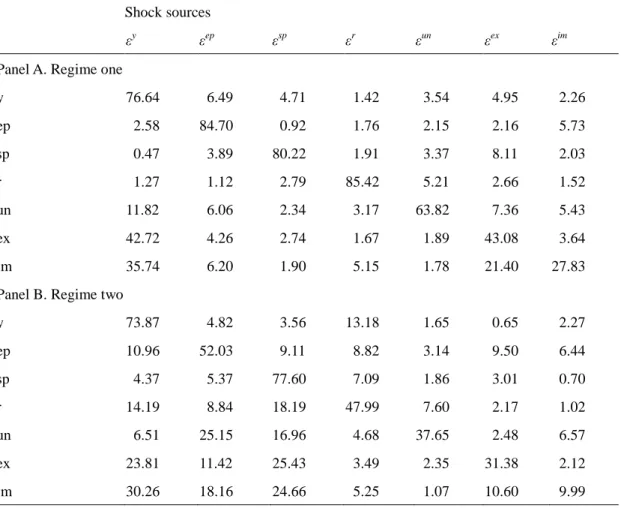
4.2.2 Results of the Variance Decomposition

Table 4.4 presents the variance decomposition results based on the VECM model for energy price. Each percentage shows how much of the unanticipated changes in macroeconomic variables are explained by the energy price variable over a 12-month horizon. The industrial production variable’s own shocks account for 77.59% to 93.95% of the forecast variance. After a year (12 months), oil prices, stock prices, interest rate, unemployment rate, exports and imports account for 1.94%, 2.72%, 1.95%, 7.55%, 5.33% and 2.91% of the industrial production forecast error variance, respectively. Compared to the other energy prices (i.e., coal price and natural gas price), oil price changes in Taiwan have the largest explanatory effect for industrial production.

After one year (12 months), 89.87% of the stock price variability is attributed to changes in itself, 1.54% to oil price changes, 2.22% to interest rate changes, and 2.75% to unemployment rate changes. Moreover, coal price changes explain a 0.22% change in stock prices, slightly lower than 0.91% explained by the interest rate. Natural gas price shocks are important driving forces behind stock price variability, explaining almost 3.53% of the variation in stock prices in the short term (about a year). The interest rate variable’s own shocks account for most of the forecast error variance. The oil price change explains about 3.88% of the interest rate change (greater than 1.64% explained by stock price change). Compared to other energy prices, a natural gas price change has stronger explanatory power on the interest rate.

For the unemployment variable, the unemployment variations are still mainly due to its own changes of about 62.77% - 81.18%, while approximately 2.52% is attributed to oil price changes, 0.40% to coal price changes, and 2.66% to natural gas price changes. In other words, a natural gas price change has stronger explanatory power on unemployment.

Table 4.4 Variance Decompositions of Forecast Error Variance in One-regime VAR Model (12 Periods Forward)

Shock sources

εy _εep _εsp _εr _εun _εex _εim

Panel A. Energy price: Oil price

y 77.59 1.94 2.72 1.95 7.55 5.33 2.91 ep 1.99 90.32 2.22 0.96 1.00 1.97 1.54 sp 1.09 1.54 89.87 2.22 2.75 0.90 1.62 r 1.50 3.88 1.64 84.49 4.02 2.48 1.99 un 20.27 2.52 1.97 2.04 66.60 3.29 3.31 ex 28.61 2.63 1.90 0.51 2.26 60.10 4.00 im 26.95 2.09 2.96 0.86 1.51 23.16 42.46

Panel B. Energy price: Coal price

y 93.95 0.52 0.14 0.08 0.27 4.97 0.09 ep 0.57 93.97 1.60 0.04 1.67 0.27 1.88 sp 0.26 0.22 95.98 0.91 1.61 0.75 0.27 r 2.33 0.96 0.86 92.80 1.48 0.35 1.22 un 14.45 0.40 0.96 0.53 81.18 0.76 1.73 ex 47.60 1.57 1.05 0.28 0.64 47.72 1.15 im 40.29 1.45 0.45 0.59 1.27 13.05 42.90

Panel C. Energy price: Natural gas price

y 81.02 0.86 2.43 2.22 2.99 8.07 2.41 ep 1.43 89.22 1.41 2.35 0.83 0.96 3.80 sp 0.80 3.53 86.41 1.58 2.79 2.56 2.38 r 1.66 1.18 1.12 86.88 4.86 2.48 1.83 un 19.98 2.66 3.58 1.22 62.77 4.48 5.31 ex 46.46 2.54 1.89 1.35 0.85 39.33 7.59 im 42.29 3.02 2.23 1.31 0.52 14.99 35.63

Note: Values in the parenthesis are standard errors estimated through 500 Monte Carlo replications. Variance decomposition explaining the variation in variables is due to industrial production shocks (εy), energy prices shocks (εep), stock price shocks (εsp), interest rate shocks (εr), unemployment rate shocks (εun), export shocks (εex), and import shocks (εim).

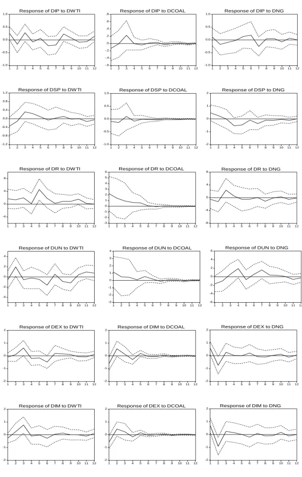
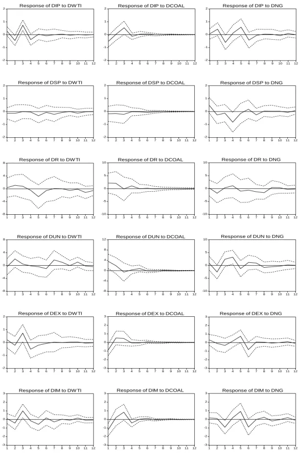
4.2.3 Results of the Impulse Response Analysis

in the system to shocks in energy prices. Figure 4.1 presents the impulse response functions of each oil price change (DWTI), coal price change (DCOAL), and natural gas price change (DNG) from one-standard deviation shocks to industrial production (DIP), stock price (DSP), real interest rates (DR), unemployment rates (DUN), exports (DEX) and imports (DIM) in the one-regime VAR model.

An oil price shock has a negative impact on industrial production. It responds negatively in period 2, and its responses exhibit more volatility. An oil price shock has a delayed negative impact on industrial production.

Following an oil price shock, stock prices decrease immediately by 0.3%, showing that an oil price shock has a negative impact on stock prices. An oil price shock has a positive impact on interest rates. The phenomenon sustains itself for approximately 12 periods. The maximum effect is reached after 4-5 periods, when the interest rate has increased by 4%. An oil price shock has a positive impact on the unemployment rate which increases by 2% in period 2.

The industrial production reacts a negatively and significantly to a coal price change in the first period. A negative response from stock prices is observed in period 2, but the effect is small and not significantly different from zero. A coal price shock always keeps a positive impact on the unemployment rate that lasts for approximately 6 periods. Following a coal price shock, both exports and imports decrease immediately by 0.5% in period 1 and then increase by 0.5% in period 2.

The industrial production decreased in periods 2 and 7 from a natural price shock. A natural gas price shock has a delayed negative impact on stock prices. With a delayed stock price response in Taiwan, stock prices at first rise and then decrease, this lasts for approximately 5-6 periods. The unemployment rate only starts to decrease in period 1 and it exhibits an upward inclination pattern in period 3.

-1.0 -0.5 0.0 0.5 1.0 1 2 3 4 5 6 7 8 9 10 11 12 Response of DIP to DW TI -.6 -.4 -.2 .0 .2 .4 .6 .8 1 2 3 4 5 6 7 8 9 10 11 12

Response of DIP to DCOAL

-1.0 -0.5 0.0 0.5 1.0 1 2 3 4 5 6 7 8 9 10 11 12 Response of DIP to DNG -1.2 -0.8 -0.4 0.0 0.4 0.8 1.2 1 2 3 4 5 6 7 8 9 10 11 12 Response of DSP to DW TI -1.0 -0.5 0.0 0.5 1.0 1 2 3 4 5 6 7 8 9 10 11 12 Response of DSP to DCOAL -2 -1 0 1 2 1 2 3 4 5 6 7 8 9 10 11 12 Response of DSP to DNG -4 0 4 8 1 2 3 4 5 6 7 8 9 10 11 12 Response of DR to DW TI -3 -2 -1 0 1 2 3 4 5 6 1 2 3 4 5 6 7 8 9 10 11 12 Response of DR to DCOAL -8 -4 0 4 8 1 2 3 4 5 6 7 8 9 10 11 12 Response of DR to DNG -4 -2 0 2 4 1 2 3 4 5 6 7 8 9 10 11 12 Response of DUN to DW TI -3 -2 -1 0 1 2 3 4 1 2 3 4 5 6 7 8 9 10 11 12

Response of DUN to DCOAL

-6 -4 -2 0 2 4 6 1 2 3 4 5 6 7 8 9 10 11 12 Response of DUN to DNG -2 -1 0 1 2 1 2 3 4 5 6 7 8 9 10 11 12 Response of DEX to DW TI -2 -1 0 1 2 1 2 3 4 5 6 7 8 9 10 11 12

Response of DIM to DCOAL

-2 -1 0 1 2 1 2 3 4 5 6 7 8 9 10 11 12 Response of DEX to DNG -2 -1 0 1 2 1 2 3 4 5 6 7 8 9 10 11 12 Response of DIM to DW TI -2 -1 0 1 2 1 2 3 4 5 6 7 8 9 10 11 12

Response of DEX to DCOAL

-2 -1 0 1 2 1 2 3 4 5 6 7 8 9 10 11 12 Response of DIM to DNG

Figure 4.1 Impulse Responses from One Standard Deviation Shock of Energy

Each macroeconomic variable should exhibit significant responses when energy price changes are modest or more. That is to say, we need to offer more detailed responses. To overcome the problem, we use the multivariate threshold error correction (MVTEC) model developed by Tsay (1998).

4.3 Two-regime VAR analysis

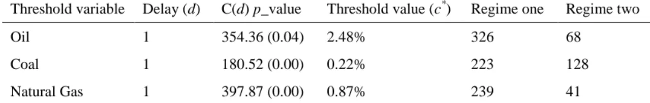
4.3.1 Estimating the Threshold Levels and the Delay of Threshold Variables

Before employing the MVTEC model, it is necessary to test the existence of the non-linear relationship in terms of the threshold variables (i.e., oil price, coal price, and natural gas price) during these two periods. The C(d) statistic based on the arranged regression (Tsay, 1998) can be used to test the linear relation. Table 4.5 displays the tests results.

Table 4.5 Results of Threshold Effect Tests

Threshold variable Delay (d) C(d) p_value Threshold value (c*) Regime one Regime two

Oil 1 354.36 (0.04) 2.48% 326 68

Coal 1 180.52 (0.00) 0.22% 223 128

Natural Gas 1 397.87 (0.00) 0.87% 239 41

Note: Regime one refers to Zt-d≤c and Regime two Zt-d≥c. c* is the optimal threshold value determined

by the location of the minimum log det|∑|, and ∑ is the variance–covariance matrix for the corresponding multivariate VECM models.

Based on Table 4.5, we can reject the null hypothesis of the linear model using oil price as a threshold variable. It means that the result favors the MVTEC model. By the same token, we find a similar result when coal price or natural gas price is used as a threshold variable. There is a non-linear relationship between energy price and industrial production. The delay (d) of the threshold variable reflects the speed of response based on the economic impact of a positive energy price change and its