用於多天線輸入多天線輸出多碼多載波系統之新型遞迴式多層級偵測技術

全文

(1)國立交通大學電信工程學系碩士班碩士論文用於多天線輸入多天線輸出多碼多載波系統之新型遞迴式多層級偵測技術 A Novel Iterative Multi-layered Detection Method for MIMO Multi-code Multicarrier Systems. 研究生指導教授. 中. 華. 民. 國. ：：. 李清凱黃家齊. 九十四. 年. 博士. 六. 月.

(2) 用於多天線輸入多天線輸出多碼多載波系統之新型遞迴式多層級偵測技術 A Novel Iterative Multi-layered Detection Method for MIMO Multi-code Multicarrier Systems 研究生：李清凱. Student ： Ching-Kai Li. 指導教授：黃家齊博士. Advisor ： Dr. Chia-Chi Huang. 國立交通大學電信工程學系碩士班碩士論文. A Thesis Submitted to Institute of Communication Engineering College of Electrical Engineering and Computer Science National Chiao Tung University in Partial Fulfillment of the Requirements for the Degree of Master of Science in Communication Engineering June 2005 Hsinchu, Taiwan, Republic of China. 中華民國九十四年六月.

(3) 用於多天線輸入多天線輸出多碼多載波系統之新型遞迴式多層級偵測技術研究生：李清凱. 指導教授：黃家齊博士. 國立交通大學電信工程學系碩士班摘要這篇論文提出在多天線輸入多天線輸出多碼多載波 (MIMO MC-MC) 系統下的一種新型遞迴式多層級偵測技術。我們推導一種簡單的適應性最小平均平方誤差等化器 (MMSE) ，且使用層級式天線干擾消除概念 (LAIC) 來減輕天線之間的相互干擾 (IAI) 並得到初始的資料偵測。接著藉由多路徑干擾消除技術達到空間分集及多路徑分集的目的。使用蒙地卡羅模擬驗證我們提出的偵測技術在多路徑衰退通道上的效能。模擬結果證實這種遞迴式多層級偵測方法在 MIMO MC-MC 系統下不只能得到高頻寬效率還能達到高功率效率。故此技術在下一代行動通訊系統中可能是一種可實行的方案。. i.

(4) A Novel Iterative Multi-layered Detection Method for MIMO Multi-code Multicarrier Systems Student: Ching-Kai Li. Advisor: Dr. Chia-Chi Huang. Institute of Communication Engineering National Chiao Tung University. Abstract This paper describes a novel iterative multi-layered detection method for MIMO multi-code multicarrier (MIMO MC-MC) system. We derive a simple adaptive minimum mean square error (MMSE) equalizer followed by a layered antenna interference cancellation (LAIC) technique to mitigate the inter-antenna interference (IAI) and obtain initial data decision. Afterwards, a multipath interference cancellation (MPIC) method is exploited to fully achieve both spatial diversity and multipath diversity. Monte Carlo simulations have been used to verify the performance of the proposed method in multipath fading channels. Simulation results demonstrate that with this iterative multi-layered detection approach, a MIMO MC-MC system is able to achieve not only high bandwidth efficiency but also high power efficiency, and it could be a good candidate for implementing the next generation mobile radio systems.. ii.

(5) 誌. 謝. 首先感謝指導教授黃家齊博士兩年來在專業知識及處事上給予學生幫助與啟示，使學生在研究態度及人生觀上有重大的改變。同時要感謝陳紹基教授及吳文榕教授對本論文的建議與指導，使學生的論文能更佳完善。. 我還要感謝古孟霖學長兩年來的熱心指導，不厭其煩地為我解惑與討論，使我能較快速的進入無線通訊的研究領域；我要感謝黃朝旺學長、鄭有財學長及劉肖真學姊在生活及課業上給予我的指導與幫助；亦要感謝陳永庭、黃俊元、林大鈞及陳韻文學長們，在找國防訓儲時給我的寶貴意見；還要感謝林永哲及黃子豪同學建構實驗室的工作站，讓我能專心從事研究；感謝研究所期間所有幫助過我的老師及同學們。. 最後更要感謝我的家人，爸爸、媽媽、大哥及二哥在我求學路上鼓勵我，支持我，使我能順利完成碩士學位。. iii.

(6) Contents. 1 Introduction. 1. 2. 5. System Model 2.1. Transmitted Signals …...……………………………... 5. 2.2. Received Signals …...………………………………... 7. 3 Iterative Multi-layered Detection Method 3.1. 10. Layered Antenna Interference Cancellation and Adaptive MMSE Equalization …...………………….. 11. 3.2. Multipath Interference Cancellation ...………………. 14. 3.3. Iterative Multi-layered Detection …...……………….. 17. 4 Simulation Results. 21. 4.1. Simulation Environments …...………………………. 21. 4.2. The Performance of MIMO MC-MC System in a Two-Path Channel …...………………………………. 4.3. The Performance of MIMO MC-MC System in the. iv. 24.

(7) Six-Path Channel …...……………………………….. 29. 5. 4.4. The Effect of Imperfect Channel Estimation …...….... 4.5. The Effect of Spatial Channel Correlation ………….. 33. Conclusion. 31. 37. Appendix A The Adaptive MMSE Equalizer. 39. Reference. 41. v.

(8) List of Figures. 2.1 The transmitter block diagram of the MIMO MC-MC system ………………………………….…….……………….... 6. 2.2 The MC-MC transmission scheme at the mth transmit antenna. 7. 2.3 The receiver block diagram of the MIMO MC-MC system at the jth receive antenna ……………………………………….. 8. 3.1 The first iteration of iterative multi-layered detection method ... 19 3.2 The second and later iterations of the iterative multi-layered detection method ………………………………………………. 20 4.1 BER performance of the MIMO MC-MC system at the first layer in the two-path channel ………………………………….. 26 4.2 Comparison between simulation results and quasi-analysis results at the first layer in the two-path channel ……………….. 27. 4.3 BER performance of the MIMO MC-MC system at all four layers in the two-path channel …………………………………. vi. 28.

(9) 4.4 BER performance of the MIMO MC-MC system at the first layer in the UMTS defined six-path channel …………………... 30. 4.5 BER performance of the MIMO MC-MC system at the first layer in the two-path channel with α as a parameter. (for the 9th iterations) ………………………………………………….. 32. 4.6 BER performance of the MIMO MC-MC system at the first layer in the spatially correlated two-path channel with ∆ as a parameter. (at the 9th iterations; Eb N 0 = 5dB ; D λ = 0.5 ; φ = 0D or 45D ) …………………………………………………….. 35. 4.7 BER performance of the MIMO MC-MC system at the first layer in the spatially correlated two-path channel with ∆ as a parameter. (at the 9th iterations; Eb N 0 = 5dB ; D λ = 10 ; φ = 0D or 45D ) …………………………………………………….. vii. 36.

(10) List of Table. 4.1 Simulation parameters …….....……………………………………... viii. 23.

(11) Chapter 1 Introduction. Over the past decade, code division multiple access (CDMA) and orthogonal frequency division multiplexing (OFDM) are two most popular transmission techniques for many commercial wireless applications, such as the third generation wideband- CDMA (WCDMA) cellular system [1] and various wireless local area networks (WLAN) [2]. A CDMA system uses spread spectrum techniques to suppress multiple access interference (MAI) and a RAKE receiver to achieve multipath diversity gains. Nevertheless, the data rate throughput is usually sacrificed for getting a large spreading factor. On the other hand, an OFDM system transforms a high rate serial data stream into multiple low rate parallel data streams to mitigate the effect of multipath interference (MPI). Besides, a one-tap equalizer, which has relatively low computation complexity, can be used by inserting a cyclic prefix (CP) at proper length.. 1.

(12) However, an OFDM system cannot achieve multipath diversity gains and it has relatively poor signal-to-noise ratio (SNR) performance due to the independent flat fading on each subcarrier. Therefore, neither the CDMA system nor the OFDM system can simultaneously achieve both high bandwidth efficiency and high power efficiency.. The demand for broadband mobile multimedia communication services will rise in the near future. Multi-code multi-carrier (MC-MC) has received significant interests and is a promising technique to fulfill high data rate multimedia communications in future cellular systems [3]-[4]. With this technique, a group of data modulated Walsh codes is transmitted over multiple subcarriers to achieve high data rate throughput. The physical channels are shared logically among users within a cell in the time domain, i.e. time division multiple access (TDMA). However, in a mobile radio environment, a multipath channel will introduce severe MPI and destroy the orthogonality among different Walsh codes. In general, this multipath phenomenon significantly degrades the data rate throughput of a multicode system. Therefore, [5]-[8] suggested a multistage multipath interference cancellation (MPIC) technique to eliminate the MPI in the received signal and achieve higher data rate throughput.. 2.

(13) Multiple input multiple output (MIMO) communication based on multiple transmit and receive antennas is another promising technique to increase bandwidth efficiency. In this approach, multiple data streams are transmitted simultaneously through different spatial channels, also known as spatial multiplexing. It was shown in [9]-[10] that the channel capacity of an MIMO system increases linearly with the minimum in the number of available transmit and receive antennas in a rich scattering environment. In general, at the receiver side, a maximum a posteriori probability (MAP) detector or maximum likelihood (ML) detector can be used to exploit the channel capacity, but with exponential power computation complexity. The Bell laboratory [11]-[12] first proposes a suboptimal layer space-time (LST) processing technique based on linear zero-forcing (ZF) spatial equalization and iterative interference cancellation. Some related research efforts [13] employing minimum mean square error (MMSE) spatial equalization instead of the ZF method is able to get better performance.. As future cellular system demands both high data rate and large area coverage which are equivalently high bandwidth efficiency and high power efficiency, respectively, a MIMO multi-code system is the most likely technology which can fulfill these two targets [14]-[19]. Nevertheless, the error rate performance of this. 3.

(14) system is heavily affected by both inter-antenna interference (IAI) and MPI. In this paper, we propose a novel iterative multilayered detection method for the MIMO MC-MC system. The signal processing chain related to each individual data stream from a transmitting antenna is referred to as a layer. A simple adaptive MMSE equalizer without matrix inversion is first applied and it is followed by a layered antenna interference cancellation (LAIC) technique to mitigate the IAI and obtain initial data decision. Afterwards, a MPIC method is adopted to achieve fully diversity gains including both spatial diversity and multipath diversity. Notable improvements can be achieved gradually after several iterations. The rest of this paper describes the principles and the performance of our proposed method is organized as follows. In Chapter 2, we describe the model of the MIMO MC-MC system, including both the transmitted and received signals. In Chapter 3, we describe our novel iterative multilayered detection method, including the LAIC concept, the adaptive MMSE equalizer, and the MPIC method. The performance of the MIMO MC-MC system is evaluated through computer simulations in Chapter 4. Finally, several conclusions are drawn in Chapter 5.. 4.

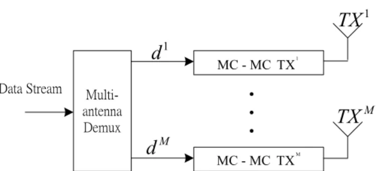
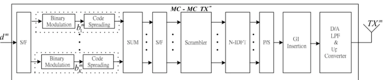
(15) Chapter 2 System Model. 2.1. Transmitted Signals. For simplicity, we assume that a MIMO MC-MC system has M antennas at both transmitter and receiver side. The transmitter block diagram of the MIMO MC-MC system is shown in Figure 2.1, a serial data stream is first serial-to-parallel (S/P) converted into M parallel data substreams d m , for 1 ≤ m ≤ M . Each data substream is then processed by an MC-MC transmission scheme and sent to the corresponding transmit antenna. Figure 2.2 shows the MC-MC transmission scheme for the mth transmit antenna. After S/P conversion, the mth data substream d m is first mapped into QPSK symbols bkm ∈ {±1 ± j} , where k denotes the kth data symbol. The data symbols are then spread by a group of Walsh codes, c k , for. 5.

(16) kaekaek. TX 1 d1 Data Stream. MC - MC TX. 1. Multiantenna Demux. TX M dM. MC - MC TX. M. Figure 2.1: The transmitter block diagram of the MIMO MC-MC system.. k = 1,… , K , where K denotes the number of Walsh codes used. Each Walsh code c k is defined as a vector c k = ⎡⎣ ck ,1 ,. , ck ,i ,. T. , ck , N ⎤⎦ , where [⋅]T denotes as the. transpose operation, N is the spreading factor, and ck ,i ∈ {1, −1} denotes the ith chip of the kth Walsh code, for 1 ≤ i ≤ N . These data modulated Walsh codes are summed up and the sum can be expressed as by a scrambling vector s m = [ s1m ,. , sim ,. ∑. K. m k =1 k k. b c . This sum is then multiplied. , sNm ]T to avoid coherent IAI at the receiver. side. As a result, the transmitted signal in frequency domain from the mth transmit antenna can be written as ⎛ K ⎞ x m = ⎜ ∑ bkmck ⎟ ⎝ k =1 ⎠ where. sm. (2.1). is the element-wise product operation.. After scrambling, an N -point inverse discrete Fourier transform (IDFT) is applied to transform the frequency domain data signal x m into a time domain data 6.

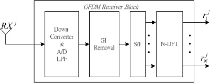
(17) kk MC - MC TX. d. m. m. TX m. b1m. bKm. Figure 2.2: The MC-MC transmission scheme at the mth transmit antenna.. signal with time duration T . A cyclically prefixed guard interval with time duration Tg is inserted to combat the inter-symbol interference (ISI) effect. Finally, the complete data signal with time duration Tg + T is converted into analog form with a digital-to-analog (D/A) converter, filtered by a low-pass filter (LPF), up converted to the radio frequency (RF) band, and transmitted in air from the mth transmit antenna.. 2.2. Received Signals. The receiver block diagram of the MIMO MC-MC system is shown in Figure 2.3. After the RF signals are received from the M receive antennas, they are first down converted to the complex equivalent baseband, low-pass filtered, and digitized. We assume that both timing and carrier frequency synchronization are perfect, and the length of the channel impulse responses of the MIMO channels are all shorter than the GI. Hence, after the GI removal, S/P conversion and N -point discrete Fourier 7.

(18) kaekaek. RX. r1 j. j. rNj. Figure 2.3: The receiver block diagram of the MIMO MC-MC system at the jth receive antenna.. transform (DFT), the received signal in frequency domain at the jth receiving antenna can be written as: M. r j = ∑ H j ,m x m + N j m =1 M. = ∑H m =1. where N j = ⎡⎣ n1j ,. r j = ⎡⎣ r1 j , , nij ,. , ri j ,. , nNj ⎤⎦. T. , rNj ⎤⎦. T. j ,m. ⎛⎛ K m ⎞ ⎜ ⎜ ∑ bk ck ⎟ ⎠ ⎝ ⎝ k =1. H j , m = diag{h0j , m ,. ,. (2.2). ⎞ s ⎟+Nj ⎠ m. , hi j ,m ,. , hNj ,m }. and. are the received signal vector, channel frequency response. matrix from the mth transmit antenna to the jth receive antenna (containing diagonal elements only), and noise vector at the jth receive antenna, respectively. The index i denotes the ith subcarrier, and 1 ≤ i ≤ N . The matrix H j ,m can be expressed as H j , m = ∑ p =1 H pj ,m in more details, where P is the total number of paths; P. H pj ,m is the channel frequency response of the pth path, which is a diagonal matrix. {. }. with each element a pj ,m exp j 2π ( i − 1)τ pj ,m N , for 1 ≤ i ≤ N , where a pj ,m and. 8.

(19) τ pj ,m are the complex fading gain and the excess delay of the pth path, respectively. The noise in each subcarrier is modeled as an independent complex Gaussian random variable with zero mean and variance σ n2 .. 9.

(20) Chapter 3 Iterative Multi-layered Detection Method. The signal processing chain related to each individual data substream from a transmit antenna is referred to as a layer. The signal processing of the Qth layer is called the Qth layered detection, hereafter. Without loss of generality, the layered detection is started with the first layer and is done in a round robin fashion. Furthermore, one complete run of all the M layered detections is called an iteration. In the following, we first describe the LAIC concept and then derive the adaptive MMSE equalizer in subsection 3.1. In subsection 3.2, we describe the MPIC method. Finally, the iterative multi-layered detection method is summarized in subsection 3.3.. 10.

(21) 3.1. Layered Antenna Interference Cancellation and Adaptive MMSE equalization. It is apparent from eq. (2.2) that the orthogonality of Walsh codes will be destroyed when the channel is frequency selective. Under such circumstances, the system encounters not only severe IAI but also severe MPI which together degrade the BER performance. Without loss of generality, we may assume that at the Qth layered detection, we have the hard decision results bˆkm of the previous. ( Q − 1). layers, for 1 ≤ m ≤ ( Q − 1) and 1 ≤ k ≤ K . Using these decision results, the IAI replicas of all the previous. ( Q − 1). data substreams can be generated and subtracted. from the received signal r j of the jth receive antenna, resulting in a signal Q −1 ⎛⎛ K ⎞ r j ,Q = r j − ∑ H j ,m ⎜ ⎜ ∑ bˆkmc k ⎟ m =1 ⎠ ⎝ ⎝ k =1. ⎞ sm ⎟ ⎠. (3.1). In general, a frequency domain adaptive MMSE equalizer G j ,Q can be applied to the signal r j ,Q to perform optimum data detection with a trade-off among MPI, IAI, residual IAI and noise. Nevertheless, the computation complexity of this optimum solution is very high due to the requirement of matrix inversion, especially when we have large number of subcarriers and antennas. Here, we consider a simple adaptive MMSE equalizer without matrix inversion, and it can be formulated by. G j ,Q = diag{g1j ,Q ,. , g i j ,Q ,. , g Nj ,Q } , for 1 ≤ i ≤ N . For simplicity, we assume that the 11.

(22) hard decision results of the previous layers are all correct, i.e. the IAI is perfectly generated and subtracted. Besides, due to the use of scrambler at the transmitter side, we can treat the unprocessed IAI as noise. Therefore, the coefficients of the adaptive MMSE equalizer can be derived as (see Appendix A). (hi j ,Q )*. g i j ,Q = hi where σ 2 = σ n2 + 2 K. M. ∑. m =Q +1. hi j ,m. 2. j ,Q 2. +. (3.2). σ2. 2K. and 1 ≤ i ≤ N ; (i)* takes complex conjugate.. Hence, the output of the frequency domain equalization through G j ,Q for the uth code channel (including also descrambling and code despreading operations) can be. (. (G. represented as cuT ⋅ sQ M. j ,Q. ). r j ,Q ) . After receiver diversity combining, we have. ( (. (G. zuQ = ∑ cuT ⋅ sQ j =1. M. j ,Q. r j ,Q ). N. M. = buQ ∑∑ gij ,Q hi j ,Q + ∑ j =1 i =1. M. M. ∑. K. K. ∑. j =1 k =1, k ≠ u. DS. +∑. )) N. bkQ (∑ gij ,Q hi j ,Q ck ,i cu ,i ) i =1. MPI. N. ∑ bkm (∑ gij ,Q hi j ,mck ,i cu ,i siQ sim ). j =1 m =Q +1 k =1. i =1. IAI M Q −1 K. N. j =1 m =1 k =1. i =1. + ∑∑∑ (bkm − bˆkm )(∑ gij ,Q hi j ,m ck ,i cu ,i siQ sim ). (3.3). RIAI M. N. + ∑∑ cu ,i gij ,Q nij siQ j =1 i =1. EN. , i.e., it consists of five components: (1) the desired data signal component, DS . (2) the MPI component, MPI , which results from the Qth data substream itself. 12.

(23) ( Q + 1) th. (3) the IAI component, IAI , which results from the. to the Mth data. substreams. (4) the residual IAI component, RIAI , which is due to the decision errors in the previous ( Q − 1) layered detections. (5) the enhanced noise component, EN . The random variables MPI , IAI , RIAI and EN all have zero mean. The variance of ℜe ( MPI ) , where ℜe ( i ) denotes the real part, can be derived and summarized as M. N. Var[ℜe ( MPI )] = ( K − 1)∑∑ ψ i j ,Q. 2. (3.4). j =1 i =1. where ψ i j ,Q = gij ,Q hi j ,Q − κ j ,Q and κ j ,Q = IDFT { gij ,Q hi j ,Q , 1 ≤ i ≤ N } . The notation. IDFT {i} denotes the value of the first point (DC value) of the N -point IDFT calculation. Besides, due to the fact that a large number of independent and identically distributed random variables are summed into the variables IAI , RIAI and EN , their variances can be calculated by using the law of large number and they are individually given by M. M. Var[ℜe ( IAI )] = K ∑. N. ∑ ∑g. j =1 m = Q +1 i =1. j ,Q i. hi j ,m. M Q −1. N. j =1 m =1. i =1. 2. Var[ℜe ( RIAI )] = 4 K ∑∑ BERm ∑ gij ,Q hi j , m. Var[ℜe ( EN )] =. σ n2 2. M. N. ∑∑ g j =1 i =1. j ,Q 2 i. (3.5) 2. (3.6) (3.7). , where BERm is the bit error rate of the mth data substream and 1 ≤ m ≤ ( Q − 1) .. 13.

(24) From eq. (3.3)-(3.7), we can calculate the mean and variance of the signal ℜe ( zuQ ) M. N. mz = ℜe {buQ } ∑∑ gij ,Q hi j ,Q. (3.8). j =1 i =1. σ z2 = Var[ℜe ( MPI )] + Var[ℜe ( IAI )] + Var[ℜe ( RIAI )] + Var[ℜe ( EN )]. (3.9). Since the variables summing up into zuQ are independent, the variable ℜe ( zuQ ) can be modeled as a Gaussian variable from the central limit theorem as M × N × K is large enough (which is true in our paper), and the conditional BER of the Qth data substream can be expressed as ⎛ m ⎞ BERQ = Φ ⎜ z ⎟ ⎜ σ2 ⎟ z ⎠ ⎝. (3.10). , where Φ ( i ) is the Q-function.. 3.2. Multipath Interference Cancellation. At the jth receive antenna and the Qth layered detection, we assume that with the hard decision results of all the other data substreams a signal r j ,Q can be obtained by subtracting the IAI from the received signal r j , that is, r j ,Q = r j −. K j ,m ⎛ ⎛ ˆm ⎞ H ⎜ ⎜ ∑ bk c k ⎟ ∑ m =1, m ≠ Q ⎠ ⎝ ⎝ k =1 M. ⎞ sm ⎟ ⎠. (3.11). With the hard decision result of the Qth data substream bˆkQ , for 1 ≤ k ≤ K , the MPIC method can be used to suppress the MPI and to achieve multipath diversity. 14.

(25) gains [5]-[8]. The detailed operations of the MPIC method are summarized as follows. First, the MPI replicas of all interfering signal paths can be generated and subtracted from the signal r j ,Q to extract the signal from each path rv j ,Q ⎛ Γ ⎛⎛ K ⎞ rv j ,Q = r j ,Q − ⎜⎜ ∑ H pj ,Q ⎜ ⎜ ∑ bˆkQ c k ⎟ ⎠ ⎝ ⎝ k =1 ⎝ p =1, p ≠ v. ⎞⎞ sQ ⎟ ⎟⎟ ⎠⎠. (3.12). , for 1 ≤ v ≤ Γ . Then, the output for the uth code channel after descrambling, code dispreading, RAKE combining, and receiver diversity combining can be calculated as: M ⎛ zuQ = ∑ cTu ⎜ sQ j =1 ⎝. Γ. ∑(H ). j ,Q H v. v =1. ⎞ rv j ,Q ⎟ ⎠. (3.13). We can detect the uth data symbol by determining whether the real part (or the imaginary part) of zuQ is greater or less than zero by hard decision. From eq. (3.11)-(3.12), for the special case of Γ = 2 , we have ⎛⎛ K ⎞ ⎛⎛ K ⎞ ⎞ r1 j ,Q = H1j ,Q ⎜ ⎜ ∑ bkQ c k ⎟ sQ ⎟ + H 2j ,Q ⎜ ⎜ ∑ bkQ − bˆkQ c k ⎟ ⎠ ⎠ ⎝ ⎝ k =1 ⎠ ⎝ ⎝ k =1 M ⎛⎛ K ⎞ ⎞ + ∑ H j , m ⎜ ⎜ ∑ bkm − bˆkm c k ⎟ s m ⎟ + N j m =1, m ≠ Q ⎠ ⎝ ⎝ k =1 ⎠. (. (. r2. j ,Q. =H +. j ,Q 2. ⎛⎛ K Q ⎞ ⎜ ⎜ ∑ bk c k ⎟ ⎠ ⎝ ⎝ k =1 M. ∑. m =1, m ≠ Q. H. j ,m. ). ⎞ sQ ⎟ ⎠. ). ⎞ ⎛⎛ K ⎞ s ⎟ + H1j ,Q ⎜ ⎜ ∑ bkQ − bˆkQ c k ⎟ ⎠ ⎠ ⎝ ⎝ k =1. (. Q. ⎛ ⎛ K m ˆm ⎞ ⎜ ⎜ ∑ bk − bk c k ⎟ ⎠ ⎝ ⎝ k =1. (. ). ). ⎞ s ⎟ ⎠ Q. ⎞ s m ⎟ +N j ⎠. From eq. (3.13) and eq. (3.14), the output of the MPIC zuQ can be expressed as. 15. (3.14).

(26) ⎧ 2 K 2 ⎛ ⎪⎪ zuQ = ∑ ⎨buQ N ∑ a pj ,Q + ∑ ⎜ bkQ − bˆkQ j =1 ⎪ p =1 k =1 ⎝ ⎪⎩ DS. (. M. +. ∑ ∑( M. K. m =1, m ≠ Q k =1. b − bˆkm m k. ). ). ⎛ a ∗ j ,Q a j ,Q e j 2π ( i −1)(τ 2j ,Q −τ1j ,Q ) 2 ℜ c c e ⎜ 1 ∑ k ,i u ,i 2 ⎝ i =1 N. ⎞⎞ ⎟⎟ ⎠⎠. RMPI. ⎛ 2 j ,Q j 2π ( i −1)τ pj ,Q c c s s ⎜ ∑ ap e ∑ i =1 ⎝ p =1 N. N. Q m k ,i u ,i i i. ∗. N. ⎞ ⎛ 2 j ,m j 2π ( i −1)τ pj ,m ⎟ ⎜ ∑ ap e ⎠ ⎝ p =1. N. ⎞ ⎟ (3.15) ⎠. RIAI. ⎛ 2 j 2π ( i −1)τ pj ,Q + ∑ cu ,i siQ nij ⎜ ∑ a pj ,Q e i =1 ⎝ p =1 N. N ⎞ ⎟ ⎠. EN. ∗. ⎫ ⎪⎪ ⎬ ⎪ ⎪⎭. , which in turn includes the desired signal component DS , the residual MPI component RMPI (resulting from the Qth data substream itself), residual IAI component RIAI (resulting from the other data substreams), and the enhanced noise component EN . The desired signal in ℜe { zuQ } is M. 2. mz = ℜe {buQ } N ∑∑ a pj ,Q. 2. (3.16). j =1 p =1. Moreover, the random variables RMPI , RIAI and EN in ℜe { zuQ } all have zero mean. The variance of ℜe { zuQ } is finally calculated as ⎧ 2 2 ⎪ σ = ∑ ⎨8 ( K − 1) N a1j ,Q a2j ,Q BERQ j =1 ⎪ RMPI ⎩ 2 z. M. ⎛ ⎛ 2⎞ 2⎞ σ ⎛ j ,Q + 4 KN ⎜ ∑ a pj ,Q ⎟ ∑ BERm ⎜ ∑ a pj ,m ⎟ + N ⎜ ∑ ap 2 ⎝ p =1 ⎝ p =1 ⎠ m =1,m ≠Q ⎝ p =1 ⎠ 2. M. 2. RIAI. 2 n. 2. EN. ⎫ 2 ⎞⎪ ⎪ ⎟⎬ ⎠⎪ ⎪⎭. (3.17). From the central limit theorem, the variable ℜe { zuQ } can be modeled as a Gaussian variable, and the conditional BER of the Qth data substream can be expressed as ⎛ m ⎞ BERQ = Φ ⎜ z ⎟ ⎜ σ2 ⎟ z ⎠ ⎝. 16. (3.18).

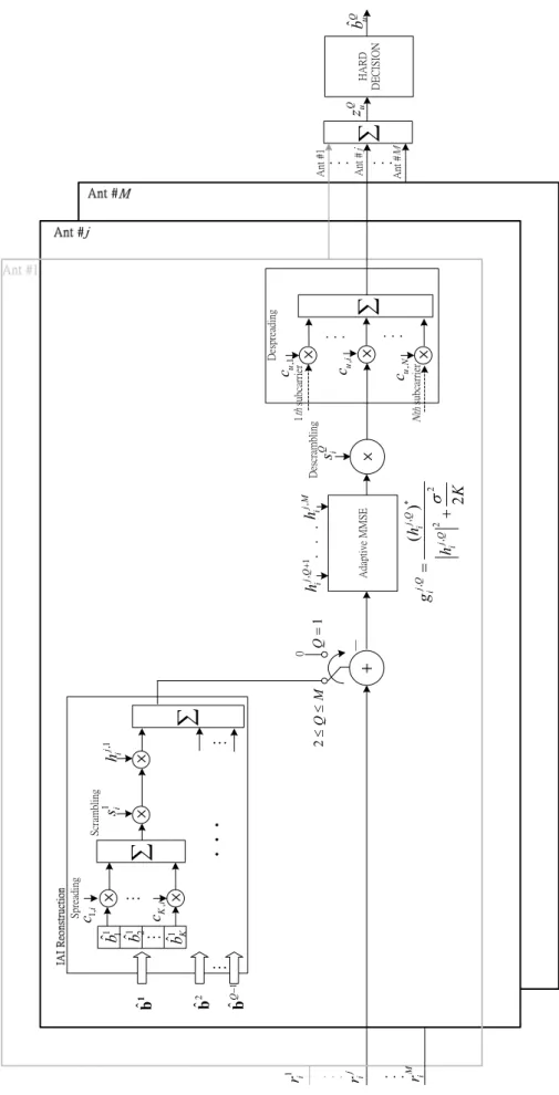
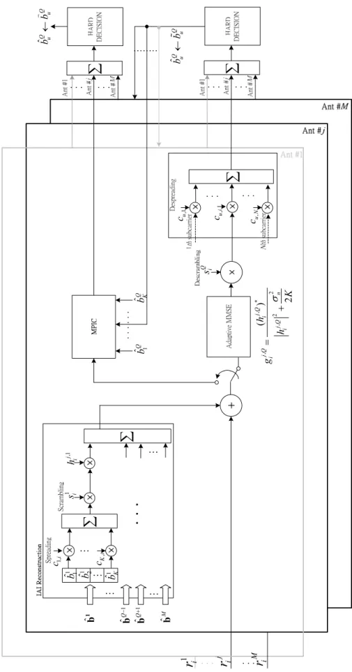
(27) 3.3. Iterative Multi-layered Detection. In this subsection, we summarize our iterative multi-layered detection method. Figure 3.1 shows the first iteration of our iterative multi-layered detection method. For the first iteration, the signal is processed according to the LAIC concept and the adaptive MMSE equalization method as described in the subsection 3.1. Note that at the first layered detection, the received signals are passed only through the adaptive MMSE equalizer to obtain the hard decision results for the first data substream.. Figure 3.2 shows the second and later iterations of the iterative multi-layered detection method. For illustration purpose, we focus on the Qth layered detection for the jth receive antenna for the second iteration. Because we have the hard decision results of all the data substreams, the LAIC eliminates all the other data substreams (excluding the Qth data substream) according to eq. (3.11) to obtain the signal r j ,Q . Afterward, we use the adaptive MMSE equalizer with coefficients of. gij ,Q = (hi j ,Q )*. (h. i. j ,Q 2. ). + σ n2 2 K , for 1 ≤ i ≤ N , to equalize the signal r j ,Q and. obtain more reliable decision result of the Qth data substream bkQ , for 1 ≤ k ≤ K . On the moment, the MPIC method mentioned in the subsection 3.2 is executed (replacing bˆkQ by bkQ ) according to eq. (3.12)-(3.13) to obtain the decision results of. 17.

(28) the Qth data substream bkQ , for 1 ≤ k ≤ K . In general, the decision result bkQ is much more accurate by fully exploiting the gain from both the spatial diversity and the path diversity. Replacing bˆkQ by bkQ in the next layered detection, the process can be repeated in several iterations until reliable data estimates of all the data substreams are obtained. Note that for the finally several iterations, the MPIC is executed alone to accelerate the convergence of BER performance.. 18.

(29) Figure 3.1: The first iteration of iterative multi-layered detection method.. 19. ri M. ri j. r. 1 i. bˆ Q−1. bˆ 2. bˆ 1. bˆK1. bˆ11 bˆ21. cK , i. ×. ×. Spreading. c1,i. ∑ ×. si1. Scrambling. ×. ∑. 2≤Q≤M. hi j ,1. Q =1. －. 0. gi. j ,Q. = hi. j ,Q 2. +. 2K. (hi j ,Q )*. σ2. hi j , M. Adaptive MMSE. hi j ,Q +1. ×. siQ. 1 Descrambling. subcarrier. cu , N. × ×. cu ,i. ∑. Despreading. cu ,1 subcarrier ×. Ant #. Ant #. Ant #1. ∑. zuQ. HARD DECISION. bûQ.

(30) Figure 3.2: The second and later iterations of the iterative multi-layered detection method.. 20. ri M. ri j. r. 1 i. bˆ M. bˆ Q−1 bˆ Q +1. bˆ 1. bˆK1. 2. bˆ11 bˆ1. cK , i. c1,i. ∑. si1 hi j ,1. ∑. gi. j ,Q. =. bˆ1Q. hi j ,Q +. 2. 2K. σ n2. (hi j ,Q )*. bˆKQ. siQ. cu , N. cu ,i. cu ,1. ∑. ∑. bûQ ← buQ. ∑. bûQ ← buQ.

(31) Chapter 4 Simulation Results. 4.1. Simulation Environments. We utilize computer simulations to verify the performance of the proposed iterative multi-layered detection method in a frequency selective channel. The equivalent baseband impulse response of the multipath channel between the mth transmit and the jth receive antenna is represented by Γ. ϒ j , m (t ) = ∑ a pj ,mδ (t − τ pj ,m ). (4.1). p =1. for 1 ≤ m, j ≤ M , where Γ is the number of resolvable paths; τ pj ,m is the excess delay of the pth path from the mth transmit antenna to the jth receive antenna; a pj , m is the complex fading gain of the pth path, which is a complex Gaussian. random variable, and δ (t ) denotes a delta function. It is assumed that the channel is. 21.

(32) stationary over each transmission. Two channel models are selected for evaluating our MIMO MC-MC system. One is a two-path channel with relative path power profiles: 0, 0 ( dB ). The other is a Universal Mobile Telecommunication System (UMTS) defined six-path channel with relative path power profiles: -2.5, 0, -12.8, -10, -25.2, -16 ( dB ) [20].. We also evaluate our MIMO MC-MC system in a spatially correlated two-path channel, which is parameterized by antenna spacing D , wavelength λ , angle of arrival (AOA) φ , and angle of spread (AOS) ∆ . For each channel path from one transmit antenna to the receiver side, the correlation of the fading patterns between receive antennas can be calculated according to [21]. Finally, in order to simulate a MIMO frequency selective fading channel, the fading patterns of each temporally resolvable path from each transmit antenna to the receive side are generated independently.. The simulation parameters for our MIMO MC-MC system are listed in Table 4.1. The entire simulations are conducted in the equivalent baseband. We assume symbol synchronization, carrier synchronization, and channel state information are perfectly estimated. The noise power is also assumed to be known at the receiver end. The. 22.

(33) kaeka Number of transmit (or receive) antennas (M). 4. Modulation. QPSK. Carrier frequency. 2 GHz. Total bandwidth. 5.12 MHz. Number of subcarriers (N). 256. Guard interval (Tg). 12.5 µ s. Length of Walsh codes (N). 256. Number of Walsh codes used (K). 256. Number of resolvable paths ( Γ ). 2 or 6. Table 4.1: Simulation parameters. Walsh codes are fully used. The scramble codes are generated from a pseudo random code with a long period and are known at the receiver end. The excess delay of the paths is uniformly distributed between 0µ s and 12.3µ s . Throughout the simulation, the parameter Eb N 0 is defined as SNR per bit per receive antenna after code despreading.. 23.

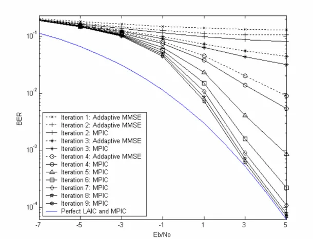
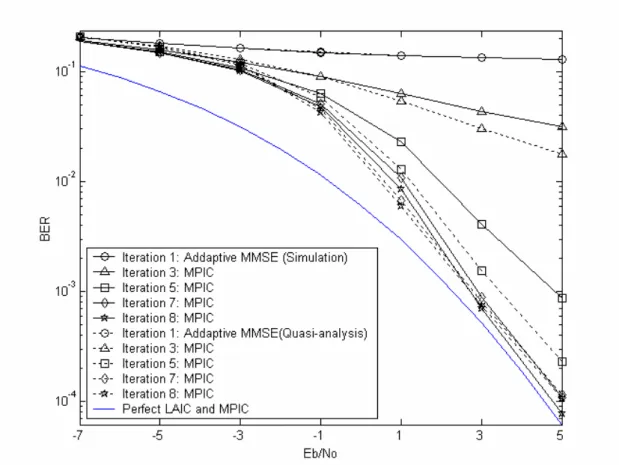
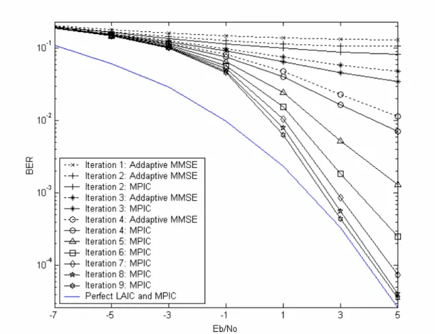
(34) 4.2. The Performance of MIMO MC-MC System in a Two-Path Channel. Figure 4.1 shows the BER performance of the MIMO MC-MC system at the first layer in the two-path channel. The BER performance for the first iteration has an error floor at BER= 10−1 because large IAI and MPI are included. For the second iteration, the BER performance is improved modestly by using adaptive MMSE and MPIC. This procedure is iterated several times (from the 2nd iteration to the 4th iteration) to obtain more and more reliable data decision results. After the 4th iteration, MPIC is executed alone to achieve full diversity gains gradually. Our simulation shows that after 9 iterations, the BER performance at high Eb N 0 approaches the theoretical limit and the degradation is only about 0.2 dB at BER= 10−3 , as compared with the case of the perfect LAIC and MPIC (i.e., the IAI and the MPI are perfectly eliminated). This simulation result shows that our iterative multi-layered detection method works well and can obtain the full benefits of both spatial diversity and path diversity.. Quasi-analysis results for BER by using the Monte Carlo method on eq. (3.10) and eq. (3.18) to average over the channel effects are shown in Figure 4.2 to verify. 24.

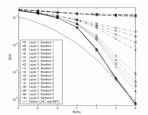
(35) our simulation results. The quasi-analysis results for BER are almost the same as the simulation results for the first three iterations. However, there is a more observable mismatch for the fifth iteration at high Eb N 0 when BER is very low, which is due to the fact that the Gaussian assumption for the residual interference components (including both IAI and MPI) is no longer valid when most interferences are reconstructed and eliminated. For the 8th iteration, the quasi-analysis results are almost consistent with the simulation results in terms of BER performance.. Figure 4.3 shows the BER performance of the MIMO MC-MC system at all four layers in the two-path channel. As shown in the figure, the Qth layered detection has a better SNR performance than the (Q − 1)th layered detection for the same iteration. These results occur because the layered detection is started with the first layer and is done in a round robin fashion. After 9 iterations, every layer finally has almost the same BER performance. In other words, the iterative multi-layered detection method is not sensitive to the order of the layer processing.. 25.

(36) Figure 4.1: BER performance of the MIMO MC-MC system at the first layer in the two-path channel.. 26.

(37) Figure 4.2: Comparison between simulation results and quasi-analysis results at the first layer in the two-path channel.. 27.

(38) Figure 4.3: BER performance of the MIMO MC-MC system at all four layers in the two-path channel.. 28.

(39) 4.3. The Performance of MIMO MC-MC System in the Six-Path Channel. Figure 4.4 shows the BER performance of the MIMO MC-MC system at the first layer in the UMTS defined six-path channel. We observe that after 9 iterations, the BER performance of the MIMO MC-MC system is degraded by only 0.5 dB and 0.2 dB at BER= 10−3 and BER= 10−4 , respectively, as compared with the case of the perfect LAIC and MPIC.. 29.

(40) Figure 4.4: BER performance of the MIMO MC-MC system at the first layer in the UMTS defined six-path channel.. 30.

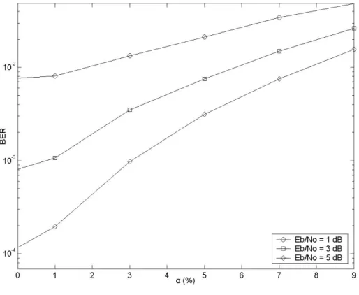
(41) 4.4. The Effect of Imperfect Channel Estimation. In the previous simulations, we assume that the channel state information is perfectly known at the receiver side. In practice, this may not be always true. In order to evaluate the effect of imperfect channel estimation, we first define a parameter of normalized channel estimation error α = ( ε Etotal ) × 100 ( % ) , where Etotal is the total channel power and ε is the power of channel estimation error. We then model the channel estimation error as follows. Let aˆ pj , m = a pj ,m + ε ρ pj ,m , where a pj ,m is actual complex fading gain defined in eq. (4.1); ρ pj ,m is a Gaussian random variable with a zero mean and unit variance and aˆ pj ,m is the channel estimation for a pj , m . Figure 4.5 shows the BER performance of the MIMO MC-MC system at the first layer in the two-path channel with α as a parameter. The simulation results show that the degradation of the BER performance is not significant for Eb N 0 = 1 dB until α = 1 , i.e. the channel power against the power of channel estimation error must be larger than 20 dB . We also observe that the BER performance is much more sensitive to the effect of imperfect channel estimation at high Eb N 0 values.. 31.

(42) Figure 4.5: BER performance of the MIMO MC-MC system at the first layer in the two-path channel with α as a parameter. (for the 9th iterations).. 32.

(43) 4.5. The Effect of Spatial Channel Correlation. The proposed system utilizes both the spatial and the path diversity gains to achieve good BER performance. We assume that the channels between receive antennas are spatially uncorrelated in the previous simulation results. In fact, the channel correlation between receive antennas depends on the parameters of antenna spacing ( D ), AOA ( φ ), AOS ( ∆ ) and wavelength ( λ ). In general, in cellular system, the antenna spacing of 0.5λ and 10λ is set (or required) in base stations and mobile terminals, respectively. Figure 4.6 and Figure 4.7 show the BER performance of the MIMO MC-MC system at the first layer in the spatially correlated two-path channel with ∆ as a parameter. The D λ is set to be 0.5 and 10 in Figure 4.6 and Figure 4.7, respectively. The Eb N 0 is 5 dB . The AOA φ is 0 or 45 . As shown in Figure 4.6, there is no significant degradation in BER performance until the AOS is smaller than 70 , which is reasonable in practical use due to the fact that large AOS is available in the environment around mobile terminals. We can also observe that the smaller the AOA is, the better the BER performance is. This is due to the fact that the spatial channel correlation is lower when the AOA is smaller. Figure 4.7 shows that there is no significant degradation in BER performance when the AOS is larger than. 15 . In real environment around base stations, the AOS is usually no more than 20 .. 33.

(44) Hence, our iterative multi-layered detection method can also perform well for uplink transmission. Finally, the BER performance is a little worse as the AOA increases.. 34.

(45) Figure 4.6: BER performance of the MIMO MC-MC system at the first layer in the spatially correlated two-path channel with ∆ as a parameter. (at the 9th iterations; Eb N 0 = 5dB ; D λ = 0.5 ; φ = 0 or 45 ).. 35.

(46) Figure 4.7: BER performance of the MIMO MC-MC system at the first layer in the spatially correlated two-path channel with ∆ as a parameter. (at the 9th iterations; Eb N 0 = 5dB ; D λ = 10 ; φ = 0 or 45 ).. 36.

(47) Chapter 5 Conclusion. The third Generation Partnership Project (3GPP) working group is now drawing up the specification of Release 7, which is an MIMO based high data rate transmission technique, for implementing the next generation mobile radio system. An MIMO MC-MC system could be a good candidate for the specification of Release 7. In this system, both the IAI and the MPI are the main factors which degrade the BER performance.. In this paper, we proposed a novel iterative multi-layered detection method for the MIMO MC-MC system to suppress both the IAI and the MPI and achieve full diversity gains. The novel iterative multi-layered detection method includes three main parts: adaptive MMSE equalization, the LAIC concept and the MPIC technique.. 37.

(48) The simple adaptive MMSE equalization and the LAIC concept are used to mitigate the severe IAI, and the MPIC method is used to combat the MPI. Our simulation results show that the system performance can be greatly improved by using the proposed iterative multi-layered detection method, and it can even approach the theoretical BER performance limit (i.e., without interference). In conclusion, the proposed iterative multi-layered detection method enables an MIMO MC-MC system to achieve simultaneously the two conflicting goals of high bandwidth efficiency and high power efficiency.. 38.

(49) APPENDIX A The Adaptive MMSE Equalizer. The received signal in frequency domain at the ith subcarrier is K. ri = hi ∑ ( dik, I + j ⋅ dik,Q ) + ni. (A-1). k =1. where hi is the channel frequency response on the ith subcarrier, dik, I + j ⋅ dik,Q is the signal spread by the ith chip of the kth Walsh code, for k = 1,… , K , and ni is the noise (including IAI) with zero mean and variance σ 2 . Moreover, the variable dik, I (or dik,Q ) has zero mean and variance 1. For simplicity, we suppose the desired. signal is d i1, I + j ⋅ di1,Q . According to the Wiener-Hopf equation, the optimum linear MMSE equalizer coefficient gi can be calculated by R ⋅ gi = P. where R is the autocorrelation of the received signal:. 39. (A-2).

(50) R = E ⎡⎣ ri ⋅ ri* ⎤⎦ * ⎡⎛ K ⎞ ⎛ K ⎞ ⎤ = E ⎢⎜ hi ∑ ( dik, I + j ⋅ dik,Q ) + ni ⎟ ⋅ ⎜ hi ∑ ( dik, I + j ⋅ dik,Q ) + ni ⎟ ⎥ ⎠ ⎝ k =1 ⎠ ⎦⎥ ⎣⎢⎝ k =1. (. ). ⎡ 2 ⎤ = E ⎢ hi ⋅ ∑ ( dik, I ) + ( dik,Q ) ⎥ +E ⎡⎣ ni ni* ⎤⎦ k =1 ⎣ ⎦ K. 2. 2. (A-3). 2. = 2 K hi + σ 2. and P is the cross-correlation between the desired signal and the received signal: P = E ⎡⎣( di1, I + j ⋅ di1,Q ) ⋅ ri* ⎤⎦ * ⎡ ⎛ K ⎞ ⎤ = E ⎢( di1, I + j ⋅ d i1,Q ) ⋅ ⎜ hi ∑ ( dik, I + j ⋅ dik,Q ) + ni ⎟ ⎥ ⎝ k =1 ⎠ ⎦⎥ ⎣⎢. (A-4). = hi* ⋅ E ⎡⎢( di1, I ) + ( di1,Q ) ⎤⎥ ⎣ ⎦ * = 2hi 2. 2. Thus, we have gi =. 2hi* 2. 2 K hi + σ 2. =. 1 ⋅ K. hi* 2. hi +. σ2. (A-5). 2K. Because the factor 1/ K is a constant, it can be neglected. We then have gi =. hi* 2. hi +. σ2 2K. 40. (A-6).

(51) Reference [1] E. Dahlman, B. Gudmundson, M. Nilsson and A. Skold, “UMTS/IMT-2000 Based on Wideband CDMA,” IEEE Commun. Mag., vol. 36, no. 9, pp. 70-80, Sept. 1998. [2] A. Doufexi, S. Armour, M. Butler, A. Nix, D. Bull, J. McGeehan and P. Karlsson, “A Comparison of the HIPERLAN/2 and IEEE 802.11a Wireless LAN Standards,” IEEE Commun. Mag., vol. 40, no. 5, pp. 172-180, May 2002. [3] A. C. McCormick and E. A. Al-Susa, “Multicarrier CDMA for Future Generation Mobile Communication,” IEE Journal on Electronics & Communication Engineering, vol. 14, no. 2, pp. 52-60, Apr. 2002. [4] R. Kimura and E. Adachi, “Comparison of OFDM and Multicode MC-CDMA in Frequency Selective Fading Channel,” Electron. Letters, vol. 39, no. 3, pp. 317-318, Feb. 2003. [5] K. Higuchi, A. Fujiwara and M. Sawahashi, “Multipath Interference Canceller for High-Speed Packet Transmission with Adaptive Modulation and Coding Scheme in W-CDMA Forward Link,” IEEE Journal on Commun., vol. 20, no. 2,. 41.

(52) pp. 419-432, Feb. 2002. [6] N. Miki, S. Abeta, H. Atarashi and M. Sawahashi, “Multipath Interference Canceller Using Soft-Decision Replica Combined with Hybrid ARQ in W-CDMA Forward Link,” in Proc. IEEE Veh. Technol. Conf., vol. 3, Oct. 2001, pp. 1922-1926. [7] T. Kawamura, K. Higuchi, Y. Kishiyama and M. Sawahashi, “Comparison Between Multipath Interference Canceller and Chip Equalizer in HSDPA in Multipath Channel,” in Proc. IEEE Veh. Technol. Conf., vol. 1, May 2002, pp. 459-463. [8] KyunByoung Ko, Dongseung Kwon, Daesoon Cho, Changeon Kang and Daesik Hong, “Performance analysis of a multistage MPIC in 16-QAM CDMA systems over multipath Rayleigh fading channels,” in Proc. IEEE Veh. Technol. Conf., vol. 4, April 2003, pp. 2807-2811. [9] G. Foschini and M. Gans, “On limits of wireless communications in a fading environment when using multiple antennas,” Wireless Pers. Comm., vol. 6, no. 3, pp. 311-335, March 1998. [10] E. Telatar, “Capacity of multi-antenna Gaussian channels,” European Trans. On Telecommun., vol. 10, no. 6, pp. 585-595, Nov./Dec. 1999. [11] G. Foschini, “Layered space-time architecture for wireless communications in a. 42.

(53) fading environment when using multi-element antennas,” Bell Labs. Tech. J., vol. 6, no.2, pp. 41-59, Autumn 1996. [12] G. Golden, C. Foschini, R. Valenzuela and P. Wolniansky,” Detection algorithm and initial laboratory results using V-BLAST space-time communication architecture,” Electron. Letters, vol. 35, no. 1, pp. 14-16, Jan. 1999. [13] Branka Vucetic and Jinhong Yuan, “Space-time coding,” Wiley, 2003. [14] M. Juntti, M. Vehkapera, J. Leinonen, V. Zexian, D. Tujkovic, S. Tsumura and S. Hara, “MIMO MC-CDMA communications for future cellular systems,” IEEE Commun. Mag., vol. 43, no. 2, pp. 118-124, Feb. 2005. [15] Haifeng Wang, Zhenhong Li and J. Lilleberg, “Equalized parallel interference cancellation for MIMO MC-CDMA downlink transmissions,” in Proc. IEEE PIMRC’03, vol. 2, Sept. 2003, pp. 1250-1254. [16] Zhongding Lei; P. Xiaoming and F. P. S. Chin, “V-BLAST receivers for downlink MC-CDMA systems,” in Proc. IEEE Veh. Technol. Conf., vol. 2, Oct. 2003, pp. 866-870. [17] P. Bouvet, V. L. Nir, M. Helard and R. L. Gouable, “Spatial multiplexed coded MC-CDMA with iterative receiver,” in Proc. IEEE PIMRC’04, vol. 2, Sept. 2004, pp. 801-804. [18] Taeyoung Kim, Kyunbyoung Ko, Sunghwan Ong, Changeon Kang and Daesik. 43.

(54) Hong, “Performance enhancement of 1x EV/DV MIMO systems in frequency selective fading channels,” in Proc. IEEE GLOBECOM’03, vol. 2, Dec. 2003, pp. 1723-1728. [19] J. Kawamoto, H. Kawai, N. Maeda, K. Higuchi and M. Sawahashi, “ Investigations on likelihood function for QRM-MLD combined with MMSE-based multipath interference canceller suitable to soft-decision turbo decoding in broadband CDMA MIMO multiplexing,” in Proc. IEEE ISSSTA’04, Sept. 2004, pp. 628-633. [20] Jonathan P. Castro, “The UMTS Network and Radio Access Technology: Air Interference Techniques for Future Mobile Systems,” New York: Wiley, 2001. [21] J. Salz and J.H. Winters, “Effect of fading correlation on adaptive arrays in digital mobile radio,” in IEEE Trans. Veh. Technol., vol. 43, no. 4, pp. 1049-1057, Nov. 1994.. 44.

(55)