土地使用政策營造的硬體面社區規模、軟體面社區管理機制、與生態社區建置及維護的因果關係研究

(1)

行政院國家科學委員會專題研究計畫成果報告

土地使用政策營造的硬體面社區規模、軟體面社區管理機

制、與生態社區建置及維護的因果關係研究

研究成果報告(精簡版)

計畫類別：個別型

計畫編號： NSC 100-2410-H-004-197-

執行期間： 100 年 08 月 01 日至 101 年 07 月 31 日

執行單位：國立政治大學地政學系

計畫主持人：蔡育新

計畫參與人員：碩士班研究生-兼任助理人員：張懿萱

碩士班研究生-兼任助理人員：白可欣

公開資訊：本計畫涉及專利或其他智慧財產權，1 年後可公開查詢

中華民國 101 年 10 月 09 日

(2)

中文摘要：都市或社區空間尺度的高密度發展，是目前用以促進交通永

續行為與減少個人平均土地消耗的重要政策，是以土地使用

政策以達成永續都市的主要政策之一。然而，高密度發展政

策的代價，是居住環境的實質條件降低，如採光、通風環

境，其對於居民、植物、或甚至動物的居住健康都可能造成

負面影響。於兼顧推動高密度發展與維持生物實質居住環境

品質兩目標下，其解決方向之一可能主要為於既有建築量體

下，提昇建物量體與開放空間於（三度）空間中的安排，亦

即如同室內家具形狀的安排、及其擺設的相關位置，以達整

體最佳的效果。然而，目前相關研究極少，缺乏提供規劃師

於上述考量的規劃目標下，制定都市規劃或設計準則時的參

考。本研究的主要目的為彙整可影響都市建物或空間安排的

都市計畫或設計工具，並量性衡量其對高密度都市環境下對

生態都市相關指標的影響。此階段以模擬分析為主的研究成

果顯示，降低建蔽率、增加高度比、以及「將退縮的樓地板

面積移往建物樓頂」，為較有效的三種都市計畫或設計工

具；衡量的生態都市指標包括友善人行空間、綠色開放空間

的可及性、二氧化碳吸收的固碳能力、以及生物多樣性指標

等。

中文關鍵詞：永續、生態都市、動物生態多樣性、都市計畫、都市設計

英文摘要： High-density development, generally at the spatial

scale of city or community, has been promoted in the

planning arena to achieve sustainable, ecological

transportation behaviour and less per capita land

consumption. However, such development may have a

negative ecological impact at the neighbourhood or

block scale in terms of natural light, wind, and the

space needed for humans, animals, and vegetation to

live healthily. One of the solutions to developing an

eco-city environment may lie in the spatial

arrangement of building mass and outdoor space；

however, few studies have been carried out in this

area. This paper presents an inventory of urban

planning and design tools for arranging building mass

and examines the impacts of these tools on eco-city

indexes. The results of simulation analyses of a

hypothetical high-density city suggest that lowering

the building coverage rate, increasing

height-distance ratio, and building setbacks with floor area

shifted to the top of the buildings are the three

(3)

most efficient tools for improving the overall

quality of eco-cities. The efficiency of the tools in

improving individual aspects of an eco-city, such as

pedestrian-friendly environment, green space

accessibility, adaptive capacity of CO2 absorption,

and animal biodiversity are also gauged.

英文關鍵詞： Sustainability, Eco-City, Animal Biodiversity, Urban

Planning, Urban Design

(4)

I

行政院國家科學委員會補助專題研究計畫

□期中進度報告

█期末報告

土地使用政策營造的硬體面社區規模、軟體面社區管理機制、與生態社區建置及

維護的因果關係研究

計畫類別：█個別型計畫 □整合型計畫

計畫編號： NSC 100-2410-H-004 -197

執行期間：2011 年 8 月 1 日至 2012 年 7 月 31 日

執行機構及系所：國立政治大學地政學系

計畫主持人：蔡育新

共同主持人：無

計畫參與人員：白可欣、張懿萱

本計畫除繳交成果報告外，另含下列出國報告，共 0 份：

□移地研究心得報告

□出席國際學術會議心得報告

□國際合作研究計畫國外研究報告

處理方式：除列管計畫及下列情形者外，得立即公開查詢

□涉及專利或其他智慧財產權，█一年□二年後可公開查詢

中華民國 10 年 10 月 8 日

(5)

I

Abstract

High-density development, generally at the spatial scale of city or community, has been promoted in the planning arena to achieve sustainable, ecological transportation behaviour and less per capita land consumption. However, such development may have a negative ecological impact at the neighbourhood or block scale in terms of natural light, wind, and the space needed for humans, animals, and vegetation to live healthily. One of the solutions to developing an eco-city environment may lie in the spatial arrangement of building mass and outdoor space; however, few studies have been carried out in this area. This paper presents an inventory of urban planning and design tools for arranging building mass and examines the impacts of these tools on eco-city indexes. The results of simulation analyses of a hypothetical high-density city suggest that lowering the building coverage rate, increasing height-distance ratio, and building

setbacks with floor area shifted to the top of the buildings are the three most efficient tools for improving the overall quality of eco-cities. The efficiency of the tools in improving individual aspects of an eco-city, such as

pedestrian-friendly environment, green space accessibility, adaptive capacity of CO2 absorption, and animal biodiversity are also gauged.

(6)

II 摘要都市或社區空間尺度的高密度發展，是目前用以促進交通永續行為與減少個人平均土地消耗的重要政策，是以土地使用政策以達成永續都市的主要政策之一。然而，高密度發展政策的代價，是居住環境的實質條件降低，如採光、通風環境，其對於居民、植物、或甚至動物的居住健康都可能造成負面影響。於兼顧推動高密度發展與維持生物實質居住環境品質兩目標下，其解決方向之一可能主要為於既有建築量體下，提昇建物量體與開放空間於（三度）空間中的安排，亦即如同室內家具形狀的安排、及其擺設的相關位置，以達整體最佳的效果。然而，目前相關研究極少，缺乏提供規劃師於上述考量的規劃目標下，制定都市規劃或設計準則時的參考。本研究的主要目的為彙整可影響都市建物或空間安排的都市計畫或設計工具，並量性衡量其對高密度都市環境下對生態都市相關指標的影響。此階段以模擬分析為主的研究成果顯示，降低建蔽率、增加高度比、以及「將退縮的樓地板面積移往建物樓頂」，為較有效的三種都市計畫或設計工具；衡量的生態都市指標包括友善人行空間、綠色開放空間的可及性、二氧化碳吸收的固碳能力、以及生物多樣性指標等。關鍵字：永續、生態都市、動物生態多樣性、都市計畫、都市設計

(7)

3

In the pursuit of sustainable or eco-city development, the high-density built environment policy of smart growth, the compact city, and transit-oriented development (TOD) has been regarded as an essential tool in urban planning (Costello, 2005). High-density residential planning is likely to degrade the residential quality of the physical environment, with opposing market and planning forces; therefore sensitive planning and design criteria and tools are necessary (Ioksin, 2010). Moreover, high-density development may harm ecological conditions such as natural light, wind, and space, which are vital to the health of the primary stakeholders of residential areas, i.e., humans, animals, and vegetation. The issue is complicated by the necessity to consider multiple ecological conditions as a whole, which unfortunately remains unresolved. Furthermore, the choice of planning and design tools available to planners and their level of influence in shaping eco-neighbourhoods have been inadequately studied in the past. This issue is particularly important for city core

residential areas, where high density makes the urban environment less healthy and enjoyable for all stakeholders.

More specifically, the challenge to the physical quality of high-density neighbourhoods may be mitigated by better urban planning and through the spatial arrangement of building mass or outdoor space. Planning and design tools include building coverage rate (BCR) and building setback (SB); however, their level of impact on ecological characteristics for all stakeholders has barely been examined. Hence, the purpose of this research is threefold: to establish an inventory of urban planning and design tools to control the built environment of a neighbourhood, to develop eco-city aspects and indexes in the urban planning realm rather than in the fields of architecture and environmental protection, and to evaluate the impacts of planning and design tools on eco-city indexes. The report includes a literature review on the eco-city, planning and design tools, eco-city indexes, and the efficiency of planning and design tools in shaping eco-neighbourhoods. It also includesresearch methods for evaluating efficiency,results of simulation analyses, and conclusions and policy implications.

1. The eco-city and urban planning and design

According to Downton (2009), there is no standard definition of the eco-city. The concept is more goal-lead than spatial-form-oriented and can be classified into three levels: less damage to the overall ecosystem of the planet in terms of resource consumption and pollution, a healthy built environment for humans, and the preservation and/or restoration of natural habitats for vegetation and wildlife. The eco-city has been advocated by environmentalists, architects, and urban planners, among others. In the arena of urban planning, eco-city implementation tools are mainly focused on land-use planning and include high–density development (Kasanko et al., 2006), mixed–use

development (Cervero et al., 2011), jobs-housing balance (Cervero, 1996a), and pedestrian-friendly environments (Cervero & Sullivan, 2011) as well as increased green space, such as parks, greenbelts,

(8)

4

and green sidewalks, to expand the ecological landscape. These large-scale spatial planning tools are intended to increase accessibility and enrich green transportation alternatives.

At the other end of the spatial-scale spectrum, green building design and materials are used by architects to increase energy efficiency and reduce the urban heat island (UHI) effect. Mid-scale neighbourhood and block planning and design tools have not been studied as much, but they appear to have the potential to achieve the goals of eco-city design from different perspectives.

Theoretically, the spatial arrangement of building mass or space in a neighbourhood determines the location, height, and/or shape of buildings, which, in turn, may affect ecological characteristics such as natural lighting (Martin & March, 1973; Yang et al., 2007), wind, the UHI effect, the

conservation of space or natural habitat for planting or wildlife, green space accessibility, and the suitability of the environment for pedestrians.

1.1 Urban planning and design tools: shaping the residential built environment

Past research, planning and design guidelines or ordinances, and case studies provide a range of tools for the arrangement of building mass at the neighbourhood level (Ioksin, 2010). For example, density distribution and open space in the land-use plan determine the large-scale or citywide building mass arrangement, whereas the spatial arrangement of building mass at the neighbourhood and block levels can be controlled by such planning and design tools as building shape (BS), floor area ratio (FAR), BCR, height distance ratio (HDR), side yard width (SW), backyard depth (BD), and SB (Taipei City Government, 2011; Brook McIlroy Planning + Urban Design, 2006).

Each of the block-level tools functions differently in arranging outdoor space or building mass. FAR determines the amount of building mass within a three-dimensional spatial unit, essentially

regulating building or population density, or both. BCR determines the extent to which ground space is reserved for such purposes as spatial openness, planting, and drainage. HDR is used to ensure daylight exposure. The stair-shaped SB (SSB) not only works as HDR but also provides more space between buildings along the street (Table 1). Moving-backwards SB (refer to Table 1 for graphic definition) leaves more street-level space as sidewalk or open space but may result in less space at the back. SW and BD can ensure the minimum distance necessary between adjoining buildings for lighting or fire prevention purposes. The location of outdoor space can be determined by building shape, such as tower, slab and cross.

1.2 Aspects and indexes of an eco-city at neighbourhood level

This section compiles the aspects and indexes of the ecological neighbourhood relevant to the three stakeholders: humans, animals, and vegetation. The first (and least complex) subsection—natural environment and adaptive capacity—concerns the extent to which the natural environment is

(9)

5

preserved in high-density urban settings, based on the assumption that the original ecological conditions are best for the native flora and fauna and, naturally, for human communities. Some natural conditions can adapt better than the built environment to environmental conditions and natural disasters; for example, large green, open space resolves the issue of surface runoff and allows the wind to blow off urban heat, and it can also provide abundant vegetation for CO2

absorption and heat mitigation. The second subsection addresses the potential for human communities to improve the environment by reducing transportation energy consumption and tailpipe pollution at the block level, which is made possible by creating a pedestrian-friendly

environment and improving green space accessibility. Unbuilt land in urban areas provides space for vegetation growth, but the natural characteristics of the land may be lost; hence the unbuilt land may serve more for humans with green environment than for plants with more natural environment to grow in. Finally, the third subsection addresses the concepts and dilemmas involved in preserving animal habitats.

1.2.1 Natural environment and adaptive capacity 1.2.1.1 Daylight exposure

Sunlight can be impeded by building mass in two ways: building height (Martin & March, 1973) and lack of permeability between buildings (Fisher-Gewirtzman et al., 2005). Conventionally, HDR is adopted as a proxy to quantify daylight exposure; however, it has the drawback of

considering only the impedance by buildings across the street. Sky view factor (SVF), defined as the ratio of sky observed to total sky hemisphere, overcomes this drawback by taking into account sunlight blocked from all directions (Ratti & Richens, 1999). Solar radiation (insolation) is a more delicate indicator, calculated on the basis of direct and diffuse radiation between the winter and summer solstice for a point location or a whole area (ESRI, 2007).

1.2.1.2 Wind environment

In urban areas, wind speed and direction can be affected by building mass, layout, height, and alignment. Earlier research has addressed the issue of discomfort caused by gusts and strong winds (American Society of Civil Engineers, 1999); however, much of the recent research in this area has focused on weak winds and public health issues such as airborne contagious disease and the UHI effect (Oke, 1982; Wong et al., 2010). Four principal measures have been applied to gauge wind speed in urban settings: field surveys, wind tunnel modeling, numerical models, and morphometric methods (Ioksin, 2010). Ground coverage ratio (GCR), defined as the ratio of total built area to total area, is proposed as a substitute for planners on the basis of its simplicity (Ng et al., 2011).

(10)

6

1.2.2.1 Pedestrian-friendly environment

Pedestrian-friendly environment, or walkability, has become more significant in achieving

sustainability due to its capacity for incubating non-mobile travel behaviour (Lo, 2009). Aside from its quantitative characteristics, its qualitative aspects include accessibility, safety, security, amenities, and diversity of pedestrians and activities. These aspects can be affected by the availability of

sidewalk, design of sidewalk network (e.g., routing and intersections) and sidewalk segments (e.g., availability of width and shade) , land use (e.g., density and diversity) and building design (e.g., front yard design) along the sidewalk, and sidewalk buffers to separate pedestrians and traffic (Ramirez et al., 2006).

1.2.2.2 Green space accessibility

Parks and community green space can meet the recreational needs of residents. Increased

accessibility to green space in a neighbourhood may reduce the distance to amenities and encourage walking and biking. There is a range of accessibility variables, each with a different emphasis and meaning (Ioksin, 2010). Euclidian distance, network distance, and travel time emphasise the closest destination as the most significant. On the other hand, the cumulative-opportunities variable

emphasises the importance of opportunities within a certain distance. More delicate, but also more difficult, variables include utilities-based (Bertolini & Kapoen, 2005), and level-of-service

accessibility indexes (Ioksin, 2010), taking both supply and demand into consideration. 1.2.3 Animals

In highly developed urban settings, two distinct dilemmas may be encountered in relation to the preservation or restoration of existing habitats. The first challenge is to develop a migration network within the limited space of a highly built environment using urban planning and design tools. The second dilemma is whether animal welfare is at risk if existing natural habitats are connected to the non-natural landscape, thereby increasing exposure to potential danger from human activities. This dilemma is addressed by two distinct planning ideologies: the biocentric equality policy proposed by Devall & Sessions (1985), which focuses on reducing exposure issue and the uncertain results of artificially created wildlife habitats, and the policy of “coexistence” of animals and humans in residential areas focusing on the re-appearance of animals in the neighborhood. Ecological condition is often measured by applying the concepts of landscape biology, i.e., the patch-corridor–matrix model (Forman and Godron, 1986), which can represent habitats, migration paths, and buildings in the context of this research.

1.3 Impacts of planning and design tools at the eco-neighbourhood level

The spatial arrangement of building mass varies depending on the planning tools used, and this is likely to affect the physical environment and the resulting ecological conditions. The impact or

(11)

7

efficiency of each planning and design tool may vary (Ioksin, 2010); for example, in a high-density neighbourhood where daylight exposure is a matter of concern, it is unclear which tool is most efficient. Furthermore, each tool is likely to affect various aspects of the physical environment differently; and evaluating their impact is further complicated when multiple aspects need to considered, with potential trade-offs between them. For instance, for the same FAR, lowered BCR can increase planting space but decrease daylight exposure, because building height increases as a result of lowered BCR.

2. Research methods

To assess the impacts of planning and design tools on eco-city building, simulation analyses are conducted for a general eco-city and for animal biodiversity. The former considers environmental sustainability from the aspects of human residents, plants, and the natural environment, but not animals; the latter focuses on developing a migration network for urban animal habitats. The hypothetical city is chosen because it provides ample scenarios of all planning and design tools, whereas in practical cases, tools are intermingled and hard to quantify. The hypothetical city

imitates the high-density city or city core since its natural environments are mostly transformed, and hence the eco-city is of more concern. All the scenarios of the hypothetical city have the same density/FAR to provide an unbiased evaluation baseline. Two analysis techniques are used: the elasticity is calculated to compare the relative efficiency of planning and design tools, and the slope is calculated to identify recommended scenarios. Google SketchUp, AutoCAD, ArcGIS, and Excel are used in the analysis.

2.1 Hypothetical city

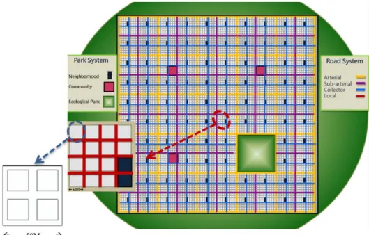
The hypothetical city designed for the eco-city simulation can be broken down into land use, road, and park systems. Its land use layout is composed of 50 m * 50 m blocks. Each block group

comprises 4 * 4 blocks, 4 * 4 block groups constitute one neighbourhood, 2.5 * 2.5 neighbourhoods constitute a community, and 2 * 2 communities constitute the 5.07 km * 5.07 km hypothetical mini-city (Figure 1), which is surrounded by natural habitats. Within each block lie four uniform buildings of the highest development density (300% FAR). These are adopted from Taipei city, which is a type IV residential area (Taipei City Government, 2011). The tower–shaped buildings have 50% BCR and 3 m storey height and face either north or south. This hypothetical city is large enough to form building clusters at its centre in order to gauge ecological indexes with little difference or distortion relative to larger cities. The land-use plan does not intentionally distinguish residential and commercial areas, etc. For simplicity, it distinguishes only between buildings and open space. Land use is served by a four-tier road hierarchy comprising 8 m local streets, 20 m

(12)

8

collectors, 30 m sub-arterial streets, and arterials (Figure 1). All but the 8 m local streets have sidewalks to simulate the situation in Taipei city.

(Figure 1 about here)

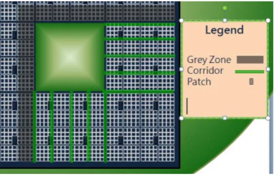
The park system, unlike other infrastructure, is incorporated into the model due to its significance ecologically and in evaluating green space accessibility. It comprises neighbourhood, community, and ecological parks wherein natural habitats remain, and it is located in the southeast quadrant (Figure 1). This quadrant is modeled in more detail for the animal-biodiversity simulation (Figure 2). The ecological park is confined by a 200-meter-wide “grey buffer” of no plants around the north and west sides and linked by some linear north-south and east-west-oriented corridors on the outskirts to minimise potential exposure to human activities. Although the network is animal-centric, the assessment of the impacts of planning tools will also apply, to a certain extent, to the policy of coexistence of animals and humans as long as the network is rewired accordingly, such as linked to other residential areas.

2.2 Urban planning and design tools and scenarios

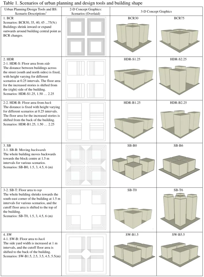
Assuming that other non-space factors such as building materials and colour are the same, six space-based urban planning and design tools are pooled together to develop various scenarios for baseline building shape (tower): BCR, HDR, SB, SW, BD, and street-corner SB (SCSB) (Table 1). In addition to the tower shape (BS1), seven other building shapes are established: enclosed

courtyard (BS2), slab (BS3), U-shaped (BS4), convex-shaped (BS5), cross-shaped (BS6), X-shaped (BS7), and reverse U-shaped (BS8). For each of the planning and design tools and building shapes, a set of scenarios is developed at fixed intervals within the largest reasonable range of variation. If possible, five scenarios are developed to calculate the efficiency/elasticity of each tool (refer to the evaluation techniques below). The descriptions and two- and three-dimensional concept graphics for the scenarios are presented in Table 1.

(Table 1 about here) 2.3 Eco-city indexes: two simulations

Eco-city indexes are developed for the general eco-city and animal-biodiversity simulation analyses, respectively. The former considers the stakeholders—residents, plants, and the natural environment and its adaptive capacity—and the latter focuses on animal migration network building. These indexes are developed to achieve a range of goals from the perspectives of the different stakeholders and also to characterise the built environment.

(13)

9

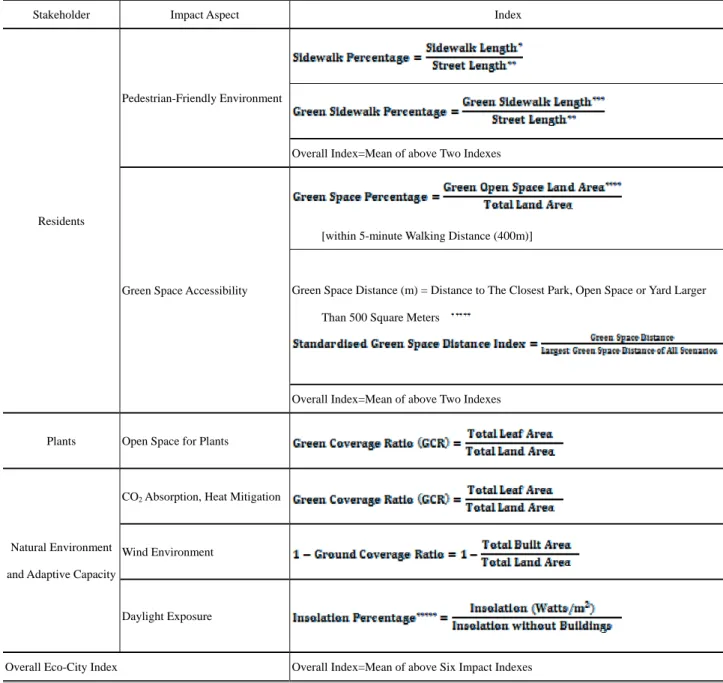
Firstly, the eco-city can be approached by reducing travel energy consumption and tailpipe pollution by creating a pedestrian-friendly environment (for trips of all purposes) and green space

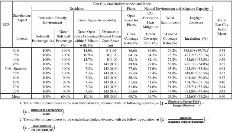
accessibility (for local recreational trips), which can also meet residents’ demands for a more natural environment (Table 2). The mean of these two indexes, equally weighted, is taken to quantify the overall pedestrian-friendly environment. The reason for the equal weighting is that the two indexes may differ under various conditions in terms of people, city, and time, and an element of arbitrary judgment is unavoidable. By the same token, this equal weighting is applied to the other aspects discussed below and to the overall physical eco-city index. Secondly, more open space for plants to grow is an eco-city goal. Thirdly, urban settings that remain closer to the original level of daylight exposure and wind environment without buildings are considered more natural for both humans and plants. Insolation, or daylight exposure, is calculated as the weighted mean magnitude of nine numeric points and four alphabetic points (Figure 4). It is measured, using ArcGIS, for residents walking on the street and at the front and back of the building on the ground level of the central block to represent the whole city. Furthermore, green space is used to quantify the city’s adaptive capacity in terms of CO2 absorption and heat mitigation. Finally, patch, T-link, and T-Gap-related

indexes are used to characterise patches and corridors for the animal-biodiversity simulation (Table 3). All the variables are standardised within the range 0–1.

(Table 2 about here)

2.4 Evaluation techniques: elasticity and slope

To evaluate the efficiency of urban planning and design tools in improving eco-city indexes, the slope and mid-point elasticity are used. The slope is primarily used to identify scenarios where the eco-city index rises or falls, representing the most significant change. Mid-point elasticity is used to cross-examine the relative efficiencies of various planning tools by taking advantage of its unit-free capacity. The elasticity is adopted and modified to measure the percentage change in an eco-city indicator as a response to the percentage change of the planning and design tool (Equation 1). The mid-point/arc elasticity is also used to calculate the average elasticity since scenarios for each planning tool cover a certain range.

(14)

10

………Equation 1

where EEC, Tool is the urban planning/design tool elasticity of the eco-city index

EC is the mid-point magnitude of the eco-city index EC is the change in magnitude of the eco-city index

Tool is the mid-point magnitude of the urban planning/design tool Tool is the change in magnitude of the urban planning/design tool 3. Impacts of urban planning and design tools on eco-city indexes

3.1 Impacts of BCR

The values of all eight indexes are presented for the eco-city aspects in Table 4-1. The statistics for pedestrian-friendly environment indexes indicate that when the BCR falls to 55%, the overall index value jumps significantly and then increases marginally, suggesting a maximum BCR of 55% in this regard. The values for sidewalk percentage show that there is enough room (the space between kerb and building wall is wider than 1.5 m (U.S. Department of Justice, 1999; Taiwan Ministry of The Interior, 2004)) to build sidewalks on both sides of the streets for all BCR scenarios (sidewalk should generally be built on the side of a road rather than on private property. However, due to the non-existence of sidewalk on most of the narrow streets in traditional residential areas in Taiwan, private property owners are encouraged to build sidewalk with a density bonus incentive.). However, the sidewalk is only wide enough (3 m) to be greened when the BCR is reduced to 55% or below. For the same reason, the accumulated percentage change in the pedestrian-friendly environment index, with a BCR of 50% as the base scenario, jumps from -50% to 0 when the BCR is reduced from 60% to 55%, that is, the highest slope (Table 4-2), indicating where the most significant impact occurs.

Based on the same analysis framework as above, the impacts of BCR on the other eco-city indexes are presented below (Tables 4-1 and 4-2). Firstly, when BCR falls from 45% to 40%, both of the green space accessibility indexes jump (the highest slope); this is because the collective open space of all four buildings in a block reaches the minimum level of a neighbourhood park for this study, i.e., 500 m2. Secondly, both the trends of index values and accumulated percentages, as well as the negative values of elasticity, show that the lower the BCR, the more space for plants to grow, and hence the higher the adaptive capacity of CO2 absorption and heat mitigation and improved wind

environment. The highest slopes suggest that the maximum BCRs for these three indexes are 55%, 55%, and 30%, respectively. Finally, the daylight exposure index shows that the impact is not linear; the highest level occurs at BCRs of 65% and 55% and the lowest occurs at both the highest and

(15)

11

lowest BCRs. This indicates that the tallest buildings with the lowest BCR of 30% and shortest buildings with the highest BCR of 75% both block the most sunlight, due to height and low permeability between buildings, respectively.

(Table 4-1 about here)

(Table 4-2 about here)

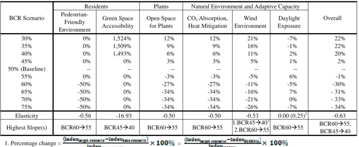
Overall, BCR is a moderately efficient planning tool for developing an eco-city; the lower the BCR, the more ecological the city. Furthermore, of all six eco-city aspects, BCR is the most efficient in the provision of green space for residents. The elasticity of overall eco-city index of -0.63 indicates that BCR is moderately (in)elastic in affecting the level of the eco-city built environment (Table 4-2). The trend of percentage changes of overall eco-city index shows that the ecological level increases as BCR decreases, and maximum BCRs of 55% and 40% are recommended for the ranges of BCR over and not greater than 40%, respectively. Of the six eco-city aspects, BCR is only elastic in affecting the accessibility to green space (Table 5-2) through the provision of a green community courtyard in the block. Though inelastic, lowering BCRs also significantly increases the levels of wind environment, pedestrian-friendly environment, open space for plants to grow, and green coverage rate for better CO2 absorption and mitigation of urban heat.

3.2

Impacts of

HDR

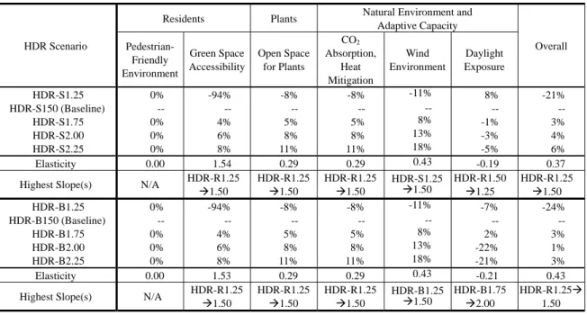
Both types of HDR are medium-efficient eco-city planning tools; the higher the HDR, the more ecological the city is, and the minimum recommended HDR is 1.5. HDR has a significant impact on green space accessibility. The elasticity values of HDR-S and HDR-B, representing the floor area added to the top of the building shifted from the side and back of the building, are 0.37 and 0.43, respectively (Table 5), less than the medium level of 0.5. The trend of the accumulated percentage change of overall eco-city index shows that the higher the HDR, and more ecological the city is. The most efficient point (i.e., the highest slope) occurs between HDR-S125 and HDR-B125 to 150; hence HDR 150 is recommended as the minimum level. This increase in open space arises because the collective backyards from the four building lots reach the minimum threshold at that point. Of the six eco-city aspects, only green space accessibility is elastic (i.e., greater than one). HDR is originally designed to ensure minimum lighting and solar radiation; however, based on the elasticity values, the increased solar radiation is achieved at a greater cost in terms of other aspects of

(16)

12

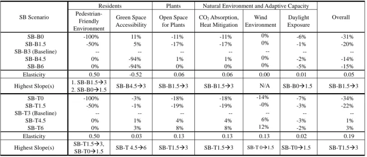
3.3 Impacts of SB

There are two types of SB, moving backwards (SB-B) and shifting floor area to the top of the building (SB-T), neither of which is a very efficient eco-city planning tool. However, the latter is slightly more efficient. A 3 m setback from the kerb is suggested as the minimum scenario to implement a greened sidewalk. Both types of SB are efficient in improving walkability, but SB-B will significantly lower green space accessibility if it downsizes the collective backyard to less than the minimum neighbourhood park size. The elasticity values of overall eco-city indexes of both types are positive but minimal, but SB-T is slightly more elastic, primarily because more open space is left on the ground (Table 6). The most efficient function of setback is providing more sidewalk space for pedestrians; therefore the accumulated percentage change in walkability jumps when the setback increases from 0 to 3 m. However, if SB-B continues to 4.5 m, the collective backyard open space becomes smaller than 500 m2.

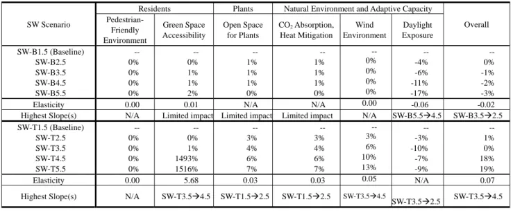
3.4 Impacts of SW and BD

Both SW types—shifting floor area to the back (SW-B) and top (SW-T) of buildings—are inefficient eco-city planning tools, with elasticity values of -0.02 and 0.07, respectively (Table 7). The suggested minimum width is 9 m, because the highest slope occurs at this point where the size of the collective backyard exceeds the threshold of 500 m2. The two types of BD—shifting floor to the side (BD-S) and to the top (BD-T) of buildings—affect the eco-city index very similarly to SW except that the distance between neighbouring buildings is shifted from the side to the back (Table 8).

3.5 Impacts of SCSB

The impacts of the two SCSB types—the horizontal (SCSB-H) and 4 m vertical (SCSB-V) setbacks—on eco-city development are minimal, but the former is slightly more efficient than the latter. For SCSB-H, the greater the street corner setback, the more ecological the city in terms of pedestrian-friendly environment, wind environment, open space for plants, CO2 absorption, and heat

mitigation. For SCSB-V, the setback at the first floor is more ecological than at the second floor and above. Both the elasticity values of overall eco-city index for both SCSB-H and SCSB–V are

(17)

13

positive but barely above zero (Table 9), but the positive value for SCSB-H indicates that the higher the horizontal setback, the more ecological the city. This type of setback, specifically designed for more spacious street corners, has limited impact overall.

3.6 Impacts of building shape

Of the eight building shapes (tower (BS1), enclosing court (BS2), slab (BS3), U-shaped (BS4), convex-shaped (BS5), cross-shaped (BS6), X-shaped (BS7), and reverse U-shaped (BS8)), tower and X-shaped buildings are, on average, the most ecological, followed by the slab shape. The tower is superior because of its capacity to provide wide sidewalks for planting trees and higher insolation derived from its compact building shape; however, the X-shaped building is supreme due to its capacity to provide greened sidewalk and to concentrate backyards to form the equivalent of neighbourhood parks. The slab shape is relatively ecological in terms of green sidewalk and improved insolation through collective open space in front and back yards. Tower, X-shaped, and slab have the three highest overall eco-city index values of 0.64, 0.63, and 0.59, respectively (Table 10). The green sidewalk percentage index also reflects that these three building shapes, in addition to cross-shaped buildings, provide sidewalk wider than 3 m for growing plants. The X-shaped is the only building shape with collective backyards larger than 500 m2, resulting in more green open space and zero distance to the nearest green open space. The tower and slab communities provide better insolation, with values of 53.4% and 54.4%, compared with 40% or below for other building shapes.

3.7 Efficiency of planning and design tools for eco-city building

To improve the overall eco-city performance of the base scenario, reducing BCR is most efficient, though only moderately elastic, followed by increasing HDR-S and HDR-B, and increasing SB by shifting floor area to the top of the building (Table 11).

In certain cases, attention may be focused on improving certain individual aspects of an eco-city. The most effective tools for improving walkability are lowering BCR and implementing building setback (Table 11). Lowering BCR overwhelms other tools in increasing green-space accessibility, followed by a second-tier of increasing SW or BD by shifting floor area to the top of the building , and a third tier of increasing HDR. The most efficient way to increase open space for plants and

(18)

14

street-level wind environment is to reduce BCR and increase HDR. Finally, if insolation is an issue for a community, reducing HDR is the most appropriate choice in accordance with existing planning knowledge.

3.8 Most ecological scenarios

Of the all of the scenarios considered, twelve have overall eco-city index values over 0.72 (Table 12). Of these twelve scenarios, only one is a non-tower building shape, i.e., X-shaped (BS 7), and the others are variations of tower-shaped buildings across five planning and design tools, consisting of large building setback with floor area shifted to the top (SB-T6, T4.5, and T3), smaller BCR (30%, 35%, and 40%), increasing side yard width by shifting floor area to top (SW-T11 and T9), increasing backyard depth by shifting floor area to top (BD-T11 and T9), and building setback by moving backward (SB-B3). All of these scenarios have streets with greened sidewalk the whole length of both sides, and a neighbourhood park equivalent is available in each block.

4. Impacts of urban planning and design tools on animal-biodiversity eco-city indexes 4.1 Impacts of BCR

Overall, BCR is an efficient tool for developing animal biodiversity in the built environment; the lower the BCR, the greater the animal biodiversity in the city. Furthermore, BCR is efficient in almost all the five indexes (Table 13). BCR levels of 40% and 55% are recommended for a positive impact on animal biodiversity.

4.2 Efficiency of planning and design tools

The most efficient tools for improving overall animal biodiversity in the built environment are lowering BCR and increasing HDR-S and HDR-B (Table 14). In terms of increasing the number of patches, lowering BCR overwhelms other tools, followed by a second-tier of SW-T and BD-T and a third tier of increasing HDR-S or HDR-B. These tools have similar impacts on the land area of patches. Where the number of corridors is of primary concern, decreasing BCR is the most efficient tool, followed by increasing SB-B and SB-T. To raise the corridor quality in terms of fewer non-green intersections, the most efficient tool is reducing BCR.

(19)

15

The twelve most efficient eco-city scenarios presented above are also the most efficient scenarios for animal biodiversity in the built environment, but in a slightly different order (Table 15). They vary only in land areas of patches and corridors, and the number of patches and corridors, as well as the quality of corridors, are the maximum afforded by the city layout.

5. Conclusions and policy implications

This research evaluates the efficiency of neighbourhood-level spatial planning and design tools for use in planning ordinances for eco-city building. Simulation analyses show that decreasing BCR is the most efficient of all the selected tools. It is efficient in almost all ecological aspects except for solar radiation, and the overall gain in all other aspects exceeds the loss in insolation. Increasing HDR is the second most efficient policy overall for eco-city building through provision of collective backyard open space between buildings, at the relatively small cost of lower insolation at the front of the building. SB-T is another relatively efficient tool in terms of providing more sidewalk space. To enhance walkability, reducing BCR and setting back buildings are the two most efficient tools. Green space accessibility can be efficiently advanced by almost all tools except street-corner building setback, as long as the building mass is shifted to the tops of buildings. To provide more space to grow plants or turf and to improve the wind environment, and consequently the adaptive capacity of CO2 absorption and heat mitigation, reducing BCR and increasing HDR are the two most

efficient tools. Similar results were found for animal diversity in the built environment, which can be applied to the intended animal immigration corridors as necessary.

Tower-shaped buildings are more ecological than other building shapes. Generally, shifting space from the ground to the top of the building, rather than to the back or side, improves ecological quality. In other words, tall, skinny buildings create more ecological neighbourhoods than short, fat buildings if the ecological aspects of this study are adopted and assigned equal importance. It is worth noting that the findings of this research are limited to a hypothetical city, which differs from practical cases in terms of shape, size, orientation, and uniformity of buildings, as well as street layout. The actual impacts of planning and design tools on a specific neighbourhood of an eco-city rely on simulation analysis.

(20)

16

References

1. American Society of Civil Engineers (1999). Wind Tunnel Studies of Buildings and Structures (Manual of Practice No. 67). Virginia: ASCE.

2. Bertolini, L. F. le Clercq and Kapoen, L. (2005). Sustainable accessibility: a conceptual framework to integrate transport and land use plan-making. Transport Policy, 12(3), 207-220.

3. Brook McIlroy Planning + Urban Design (2006). City of Burlington: Downtown Urban Design

Guidelines [online]. Available from: http://cms.burlington.ca/AssetFactory.aspx?did=4976

(Accessed 30 January 2012).

4. Camagni, R., Gibelli, M.C. and Rigamonti, P. (2002). Urban mobility and urban form: the social and environmental costs of different patterns of urban expansion. Ecological Economics, 40(2), 199–216.

5. Cervero, R. (1996). Mixed land uses and commuting: Evidence from the American Housing

Survey. Transportation Research Part A: Policy and Practice, 30(5), 361–377.

6. Cervero, R., Ewing, R., Greenwald, M., Zhang, M., Walters, J., Feldman, M., Frank, L. and Thomas, J. (2011). Traffic generated by mixed-use developments—six-region study using consistent built environmental measures. Journal of Urban Planning and Development, 137(3), 248–261.

7. Cervero, R. and Sullivan, C. (2011). Green TODs: Marrying transit-oriented development and green urbanism. International Journal of Sustainable Development & World Ecology, 18(3), 210–218.

8. Costello, L. (2005). From prisons to penthouses: The changing images of high-rise living in Melbourne. Housing Studies, 20(1), 49–62.

9. Devall, B. and Sessions, G. (1985). Deep Ecology: Living As If Nature Mattered. Salt Lake City: G. M. Smith.

10. Downton, P. F. (2009). Ecopolis: Architecture and Cities for a Changing Climate. Collingwood, Australia: CSIRO Publishing.

11. Environmental Systems Research Institute, Inc. (ESRI) 2007. Calculating Insolation.

http://cms.burlington.ca/AssetFactory.aspx?did=4976.http://webhelp.esri.com/arcgisdesktop/9. 2/index.cfm?TopicName=Calculating_solar_radiation.

12. Fisher-Gewirtzman, D., Pinsly, D.S., Wagner, I.A. and Burt, M. (2005). View-oriented three-dimensional visual analysis models for the urban environment. Urban Design

(21)

17

International, 10(1), 23–37.

13. Forman, R.T.T. and Godron, M. (1986). Landscape Ecology. New York: John Wiley & Sons. 14. Kasanko, M., Barredo, J.I., Lavalle, C., McCormick, N., Demicheli, L., Sagris, V. and Brezger,

A. (2006). Are European cities becoming dispersed? A comparative analysis of fifteen European urban areas. Landscape and Urban Planning, 77, 111–130.

15. Lo, R.H. (2009). Walkability: what is it? Journal of Urbanism, 2(2), 145–166.

16. Martin, L. and March, L. (eds.) (1973). Urban Space and Structures. Cambridge: Cambridge University Press.

17. Ng, E., Chao, Y., Liang, C., Chao, R. and Jimmy, C.H.F. (2011). Improving the wind

environment in high-density cities by understanding urban morphology and surface roughness: A study in Hong Kong. Landscape and Urban Planning, 101, 59–74.

18. Oke, T.R. (1982). The energetic basis of the urban heat island. Quarterly Journal of the Royal

Meteorological Society, 108, 1–24.

19. Ramirez, L.K.B., Hoehner, C.M., Brownson, R.C., Cook, R., Orleans, C.T., Hollander, M., Barker, D.C., Bors, P., Ewing, R., Killingsworth, R., Petersmarck, K., Schmid, T. and Wilkinson, W. (2006). Indicators of activity-friendly communities: An evidence-based consensus process. American Journal of Preventive Medicine, 31(6), 515–524.

20. Ratti, C., & Richens, P. (1999). Urban texture analysis with image processing techniques, in

Computers in Building: Proceedings of the CAADfutures’99 Conference. USA: Kluwer

Academic Publishers, 49–64.

21. Taipei City Government (2011). Taipei City zoning ordinance [online, in Chinese]. Available from: http://www.udd.taipei.gov.tw/pages/detail.aspx?Node=46&Page=2102&Index=5

(Accessed 2009).

22. Taipei City Government (2011). Demographical Overview [online]. Available from:

http://english.taipei.gov.tw/ct.asp?xItem=1084529&ctNode=29491&mp=100002 (Accessed 18 August 2011).

23. Taiwan Ministry of The Interior. (2004). Guidelines for Sidewalk Design in Urban Settings.

Taipei: Minister of Interior[online, in Chinese]. Available from:

http://w3.cpami.gov.tw/district6/i5.htm (Accessed 20 January 2011).

24. Ioksin, Y.H. (2010). Urban Planning/Design Tools for Improving Physical Aspects of Livability in High-Density Neighborhoods. 2011 International Winter Conference on Environmental Innovations and Sustainability. 28 and 29 January, 2011. Beppu, Oita, Japan. 25. U.S. Department of Justice. (1999). Americans with Disabilities Act. Accessible Rights-of-Way:

(22)

18

A Design Guide [online]. Available from

http://www.access-board.gov/prowac/guide/PROWGuide.htm (Accessed 20 January 2011). 26. Wong, M.S., Nichol, J. E., To, P.H. and Wang, J. (2010). A simple method for designation of

urban ventilation corridors and its application to urban heat island analysis. Building and

Environment, 45, 1880–1889.

27. Yang, P.P.J., Putra, S.Y. and Li, W.J. (2007). Viewsphere: a GIS-based 3D visibility analysis for urban design evaluation. Environment and Planning B: Planning and Design, 43, 971–992.

List of Figures

Figure 1. Base map of hypothetical city for general eco-city simulation analysis

Figure 2. Hypothetical community for animal-biodiversity simulation analysis

Figure 3. Sampling points for measuring insolation

(23)

19

(24)

20

(25)

21

(26)

22

List of Tables

Table 1. Scenarios of urban planning and design tools and building shape

Table 2. Eco-city indexes for general eco-city simulation, by stakeholder and by impact

aspect

Table 3. Eco-city indexes for animal-biodiversity simulation, by aspect

Table 4-1. Eco-city indexes, BCR

Table 4-2. Accumulated percentage change,

elasticity, and slope of eco-city index, BCR

Table 5. Accumulated percentage change, elasticity, and slope of eco-city indexes, HDR

Table 6. Accumulated percentage change, elasticity, and slope of eco-city indexes, SB

Table 7. Accumulated percentage change, elasticity, and slope of eco-city indexes, SW

Table 8. Accumulated percentage change, elasticity, and slope of eco-city indexes, BD

Table 9. Accumulated percentage change, elasticity, and slope of eco-city indexes, SCSB

Table 10. Eco-city indexes, BS

Table 11. Elasticity of urban design tools

Table 12. Most ecological scenarios

Table 13. Animal-biodiversity eco-city indexes, BCR

Table 14. Elasticity of animal-biodiversity eco-city indexes

Table 15. Most animal-biodiversity built environment scenarios

(27)

23

Table 1. Scenarios of urban planning and design tools and building shape

Urban Planning/Design Tools and BS: Scenario Descriptions1

2-D Concept Graphics:

Scenarios (Overlaid) 3-D Concept Graphics 1. BCR

Scenarios: BCR30, 35, 40, 45 ...75(%) Buildings shrink inward or expand outwards around building central point as BCR changes.

BCR30 BCR75

2. HDR

2-1. HDR-S: Floor area from side The distance between buildings across the street (south and north sides) is fixed, with height varying for different scenarios at 0.25 intervals. The floor area for the increased stories is shifted from the (right) side of the building. Scenarios: HDR-S1.25, 1.50 … 2.25

HDR-S1.25 HDR-S2.25

2-2. HDR-B: Floor area from back The distance is fixed with height varying for different scenarios at 0.25 intervals. The floor area for the increased stories is shifted from the back of the building. Scenarios: HDR-B1.25, 1.50 … 2.25

HDR-B1.25 HDR-B2.25

3. SB

3-1. SB-B: Moving backwards The whole building moves backwards towards the block centre at 1.5 m intervals for various scenarios. Scenarios: SB-B0, 1.5, 3, 4.5, 6 (m)

SB-B0 SB-B6

3-2. SB-T: Floor area to top

The whole building shrinks towards the south-east corner of the building at 1.5 m intervals for various scenarios, and the cutoff floor area is shifted to the top of the building.

Scenarios: SB-T0, 1.5, 3, 4.5, 6 (m)

SB-T0 SB-T6

4. SW

4-1. SW-B: Floor area to back The side yard width is increased at 1 m intervals, and the cutoff floor area is shifted to the back of the building. Scenarios: SW-B1.5, 2.5, 3.5, 4.5, 5.5(m)

(28)

24

4-2. SW-T: Floor area to top

The side yard width is increased at 1 m intervals, and the cutoff floor area is shifted to the top of the building. Scenarios: SW-T1.5, 2.5, 3.5, 4.5, 5.5 (m)

SW-T1.5 SW-T5.5

5. BD

5-1. BD-S: Floor area to side The backyard depth is increased at 1 m intervals, and the cutoff floor area is shifted to the right side of the building. Scenarios: BD-S1.5, 2.5, 3.5, 4.5, 5.5 (m)

BD-S1.5 BD-S5.5

5-2 BD-T: Floor area to top

The backyard depth is increased at 1 m intervals, and the cutoff floor area is shifted to the top of the building. Scenarios: BD-T1.5, 2.5, 3.5, 4.5, 5.5 (m)

BD-T1.5 BD-T5.5

6. SCSB

6-1. SCSB-H-1F: Horizontal setback on 1F

The building corner at the intersection is set back from the ground level and 0, 2, 4, and 6 meters above for various scenarios, and the cutoff floor area is shifted to the top of the building. This can also be called horizontal setback. Scenarios: SCSB-H-1F0M, 2M, 4M, 6M

SCSB-H-1F0M SCSB-H-1F4M

6-2. SCSB-V-4M: Vertical 4 m setbacks The building corner at the intersection is set back for 4 meters starting from 3F, 2F, and 1F for various scenarios, and the cutoff floor area is shifted to the top of the building. This can also be called vertical setback.

Scenarios: SCSB- V-4M-None, 3F, 2F, 1F

SCSB-V-4M1F SCSB-V-4M2F

7. BS

BS2. Enclosed courtyard The front yard depths for various scenarios are 1.5, 2, 2.5, and 3 m; the cutoff floor area is moved into the courtyard.

Scenarios: BS2-1.5, 2, 2.5, 3 (m)

(29)

25

BS3. Slab

The side yard widths for various scenarios are 1 and 2 m. Scenarios: BS3-1, 2 (m)

BS3-1 BS3-2

BS4. U-Shaped

The depths of the pits of the U-shaped buildings vary at 1 m intervals. Scenarios: BS4-1, 2, 3 (m)

BS4-1 BS4-3

BS5. Convex-shaped

The lengths of the front bulges of the convex-shaped buildings vary at 1 m intervals.

Scenarios: BS5-1, 2, 3 (m)

BS5-1 BS5-3

BS6. Cross-shaped

The lengths of the four arms of the cross-shaped buildings vary at 0.5 m intervals.

Scenarios: BS6-2, 2.5, 3 (m)

BS6-2 BS6-3

BS7. X-shaped

The lengths of the leg parts of the buildings vary at 0.5 m intervals. Scenarios: BS7-2, 2.5, 3 (m)

BS7-2 BS7-3

BS8. Reverse U-shaped The depths of the dent parts of the buildings vary at 1 m intervals. Scenarios: BS8-1, 2, 3 (m)

BS8-1 BS8-3

(30)

26

Table 2. Eco-city indexes for general eco-city simulation, by stakeholder and by impact aspect

Stakeholder Impact Aspect Index

Residents

Pedestrian-Friendly Environment

Overall Index=Mean of above Two Indexes

Green Space Accessibility

[within 5-minute Walking Distance (400m)]

Green Space Distance (m) = Distance to The Closest Park, Open Space or Yard Larger

Than 500 Square Meters

Overall Index=Mean of above Two Indexes

Plants Open Space for Plants

Natural Environment

and Adaptive Capacity

CO2 Absorption, Heat Mitigation

Wind Environment

Daylight Exposure

Overall Eco-City Index Overall Index=Mean of above Six Impact Indexes

* Sidewalk length is the total length of the street segments where the width between the kerb and building façade is larger than 1.5 m for installation of minimal sidewalk.

** The street length excludes the intersection segments, where sidewalk cannot be implemented.

*** Green sidewalk length is the total length of the street segments where the width between kerb and front wall of the building is larger than 3 m, allowing trees or turf to be grown on the sidewalk.

**** Green open space is defined as those parks, open spaces, or yards larger than 500 m2_{, which is the most popular park size (500–1000 m}2_{) and}

the bottom 15.4-percentile of parks of the Taipei city land-use plan.

***** The location setting is Taipei city, and the time period is the second half of the year 2011, between the first day of summer and the last day of fall.

(31)

27

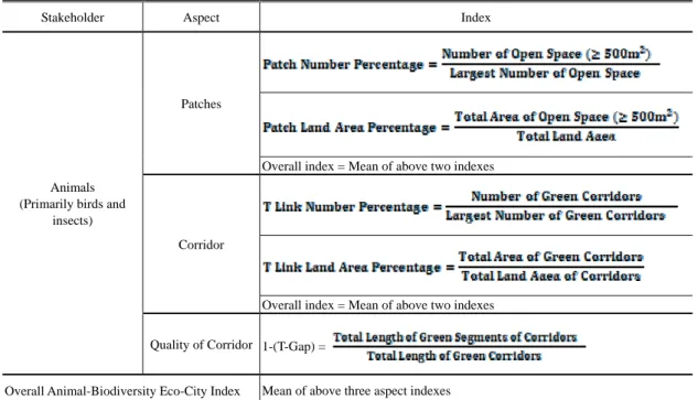
Table 3. Eco-city indexes for animal-biodiversity simulation, by aspect

Stakeholder Aspect Index

Animals (Primarily birds and

insects)

Patches

Overall index = Mean of above two indexes

Corridor

Overall index = Mean of above two indexes

Quality of Corridor 1-(T-Gap) =

(32)

28

Table 4-1. Eco-city indexes, BCR

BCR

Eco-City Stakeholder/Aspect and Index

Stakeholder/ Aspect

Residents Plants Natural Environment and Adaptive Capacity

Overall Eco-City

Index (Mean) Pedestrian-Friendly

Environment Green Space Accessibility

Open Space for Plants CO2 Absorption, Heat Mitigation Wind Environment Daylight Exposure Indexes Sidewalk Percentage (%) Green Sidewalk Percentage (%) Green Open Space Percentage within 5-Minute Walk (%) Distance to Nearest Green Open Space (m) Green Coverage Ratio (%) Green Coverage Ratio (%) 1-Ground Coverage Ratio (%) (%) 30% 100% 100% 18.0% 0 (1.00)1 86.6% 86.6% 79.2% 395,808 (49.7%)2 0.78 35% 100% 100% 16.9% 0 (1.00) 84.3% 84.3% 75.7% 423,215 (53.1%) 0.77 40% 100% 100% 15.7% 0 (1.00) 82.1% 82.1% 72.2% 432,619 (54.3%) 0.76 45% 100% 100% 7.3% 143 (0.00) 79.8% 79.8% 68.8% 430,112 (54.0%) 0.65 50% (Baseline) 100% 100% 7.3% 143 (0.00) 77.6% 77.6% 65.3% 425,599 (53.4%) 0.64 55% 100% 100% 7.3% 143 (0.00) 75.4% 75.4% 61.8% 449,875 (56.5%) 0.63 60% 100% 0.0% 7.3% 143 (0.00) 56.4% 56.4% 58.3% 404,469 (50.8%) 0.47 65% 100% 0.0% 7.3% 143 (0.00) 51.6% 51.6% 54.9% 454,768 (57.1%) 0.46 70% 100% 0.0% 7.3% 143 (0.00) 51.6% 51.6% 51.4% 425,711 (53.4%) 0.44 75% 100% 0.0% 7.3% 143 (0.00) 51.6% 51.6% 47.9% 393,897 (49.4%) 0.43 Mean 100% 60.0% 10.1% 100 (0.30) 69.7% 69.7% 63.5% 423,607 (53.2%) 0.60

1. The number in parentheses is the standardised index, obtained with the following equation =

(33)

29

Table 4-2. Accumulated percentage change,1 elasticity, and slope of eco-city index, BCR

BCR Scenario

Overall Pedestrian- Friendly Environment Green Space Accessibility Open Space for Plants CO2 Absorption, Heat Mitigation Wind Environment Daylight Exposure 30% 0% 1,524% 12% 12% 21% -7% 22% 35% 0% 1,509% 9% 9% 16% -1% 22% 40% 0% 1,493% 6% 6% 11% 2% 20% 45% 0% 0% 3% 3% 5% 1% 2% 50% (Baseline) -- -- -- -- -- -- -- 55% 0% 0% -3% -3% -5% 6% -1% 60% -50% 0% -27% -27% -11% -5% -30% 65% -50% 0% -34% -34% -16% 7% - 31% 70% -50% 0% -34% -34% -21% 0% - 33% 75% -50% 0% -34% -34% -26% -7% - 34% Elasticity -0.56 -16.93 -0.50 -0.50 -0.53 0.00 (0.25)2_-0.63 Highest Slope(s) BCR6055 BCR4540 BCR6055 BCR6055 1.BCR4540 3 2.BCR6055 BCR6055 BCR6055, BCR4540 1. Percentage change = =

2. The impact of BCR on solar radiation is not linear; it peaks at BCRs of 55% and 65% and is lower at both ends. An alternative, gauging the elasticity between BCRs of 55% and 30%, shown in the parentheses, is provided.

3. For those with more than two highest slopes, the one with the highest index value is prioritised since it is more ecological.

(34)

30

Table 5. Accumulated percentage change, elasticity, and slope of eco-city indexes, HDR

HDR Scenario

Residents Plants Natural Environment and Adaptive Capacity Overall Pedestrian- Friendly Environment Green Space Accessibility Open Space for Plants CO2 Absorption, Heat Mitigation Wind Environment Daylight Exposure HDR-S1.25 0% -94% -8% -8% -11% 8% -21% HDR-S150 (Baseline) -- -- -- -- -- -- -- HDR-S1.75 0% 4% 5% 5% 8% -1% 3% HDR-S2.00 0% 6% 8% 8% 13% -3% 4% HDR-S2.25 0% 8% 11% 11% 18% -5% 6% Elasticity 0.00 1.54 0.29 0.29 0.43 -0.19 0.37 Highest Slope(s) N/A HDR-R1.25_1.50 HDR-R1.25_1.50 HDR-R1.25_1.50 HDR-S1.25_1.50 HDR-R1.50_1.25 HDR-R1.25_1.50

HDR-B1.25 0% -94% -8% -8% -11% -7% -24% HDR-B150 (Baseline) -- -- -- -- -- -- -- HDR-B1.75 0% 4% 5% 5% 8% 2% 3% HDR-B2.00 0% 6% 8% 8% 13% -22% 1% HDR-B2.25 0% 8% 11% 11% 18% -21% 3% Elasticity 0.00 1.53 0.29 0.29 0.43 -0.21 0.43 Highest Slope(s) N/A HDR-R1.25_1.50 HDR-R1.25_1.50 HDR-R1.25_1.50 HDR-B1.25_1.50 HDR-B1.75_2.00 HDR-R1.25

(35)

31

Table 6. Accumulated percentage change, elasticity, and slope of eco-city indexes, SB

SB Scenario

Overall Pedestrian- Friendly Environment Green Space Accessibility Open Space for Plants CO2 Absorption, Heat Mitigation Wind Environment Daylight Exposure SB-B0 -100% 11% -11% -11% 0% -6% -31% SB-B1.5 -50% 5% -17% -17% 0% -1% -20% SB-B3 (Baseline) -- -- -- -- -- -- -- SB-B4.5 0% -94% 1% 1% 0% -2% -14% SB-B6 0% -94% 0% 0% 0% -5% -15% Elasticity 0.50 -0.52 0.06 0.06 0.00 0.01 0.05 Highest Slope(s) 1. SB-B1.53 2. SB-B01.5 SB-B4.53 SB-B1.53 SB-B1.53 N/A SB-B01.5 SB-B1.53 SB-T0 -100% -3% -18% -18% -14% -7% -34% SB-T1.5 -50% -1% -19% -19% -0% -3% -22% SB-T3 (Baseline) -- -- -- -- -- -- -- SB-T4.5 0% 1% 4% 4% 6% -3% 1% SB-T6 0% 3% 8% 8% 12% -2% 3% Elasticity 0.50 0.03 0.13 0.13 0.13 0.02 0.19 Highest Slope(s) SB-T1.53, SB-T01.5 SB-T 4.56 SB-T1.53 SB-T1.53 SB-T 01.5 SB-T01.5 SB-T1.53

(36)

32

Table 7. Accumulated percentage change, elasticity, and slope of eco-city indexes, SW

SW Scenario

Overall Pedestrian- Friendly Environment Green Space Accessibility Open Space for Plants CO2 Absorption, Heat Mitigation Wind Environment Daylight Exposure SW-B1.5 (Baseline) -- -- -- -- -- -- -- SW-B2.5 0% 0% 1% 1% 0% -4% 0% SW-B3.5 0% 1% 1% 1% 0% -6% -1% SW-B4.5 0% 1% 1% 1% 0% -11% -2% SW-B5.5 0% 2% 0% 0% 0% -17% -3%

Elasticity 0.00 0.01 N/A N/A 0.00 -0.06 -0.02 Highest Slope(s) N/A Limited impact Limited impact Limited impact N/A SW-B5.54.5 SW-B3.52.5

SW-T1.5 (Baseline) -- -- -- -- -- -- -- SW-T2.5 0% 0% 3% 3% 3% -3% 1% SW-T3.5 0% 1% 4% 4% 6% -10% 0% SW-T4.5 0% 1493% 6% 6% 10% -7% 18% SW-T5.5 0% 1516% 7% 7% 13% -9% 19% Elasticity 0.00 5.68 0.03 0.03 0.05 N/A 0.07 Highest Slope(s) N/A SW-T3.54.5 SW-T1.52.5 SW-T1.52.5 SW-T3.54.5

(37)

33

Table 8. Accumulated percentage change, elasticity, and slope of eco-city indexes, BD

BD Scenario

Overall Pedestrian- Friendly Environment Green Space Accessibility Open Space for Plants CO2 Absorption, Heat Mitigation Wind Environment Daylight Exposure BD-S1.5(Baseline) -- -- -- -- -- -- -- BD-S2.5 0% 0% 1% 1% 0% 6% 1% BD-S3.5 0% 1% 1% 1% 0% 12% 2% BD-S4.5 0% 1% 1% 1% 0% 15% 3% BD-S5.5 0% 1% 0% 0% 0% 19% 3% Elasticity 0.00 0.00 0.00 0.00 0.00 0.07 0.02

Highest Slope(s) N/A Limited impact

Limited

impact Limited impact N/A

1. BD-S2.53.5, 2. BD-S1.52.5, 1. BD-S3.54.5, 2. BD- S2.53.5 BD-T1.5 (Baseline) -- -- -- -- -- -- -- BD-T2.5 0% 0% 3% 3% 3% 5% 2% BD-T3.5 0% 0% 4% 4% 6% 0% 2% BD-T4.5 0% 1478% 6% 6% 10% 8% 21% BDT-5.5 0% 1501% 7% 7% 13% 7% 22% Elasticity 0.00 5.63 0.03 0.03 0.05 0.03 0.08

(38)

34

Table 9. Accumulated percentage change, elasticity, and slope of eco-city indexes, SCSB

SCSB Scenario

Residents Plants Natural Environment and Adaptive Capacity

Overall Pedestrian- Friendly Environment Green Space Accessibility Open Space for Plants CO2 Absorption, Heat Mitigation Wind

Environment Solar Radiation

SCSB-H-1F0M (Baseline) -- -- -- -- -- -- SCSB-H-1F2M 3% 0% 0% 0% 1% 6% 2% SCSB-H-1F4M 7% 0% 1% 1% 3% 5% 3% SCSB-H-1F6M 11% 0% 3% 3% 6% 3% 4% Elasticity 0.04 0.00 0.01 0.01 0.02 N/A 0.02 Highest Slope(s) SCSB-H-1F4M _1F6M N/A SCSB-H-1F4M _1F6M SCSB-H-1F4M _1F6M SCSB-H-1F4M _1F6M SCSB-H-1F2M SCSB-H-1F0M_1F2M SCSB-V-4M-None (Baseline) -- -- -- -- -- -- SCSB-V-4M3F 0% 0% 0% 0% 0% 8% 1% SCSB-V-4M2F 0% 0% 0% 0% 0% 8% 1% SCSB-V-4M1F 7% 0% 2% 2% 3% 5% 3% Elasticity 0.02 0.00 0.01 0.01 0.01 N/A 0.01 Highest Slope(s) SCSB-V-4M2F _4M1F N/A SCSB-V-4M2F _4M1F SCSB-V-4M2F_4M1F SCSB-V-4M2F _4M1FSCSB-V- 4M3F, _-4M2F SCSB-V-4M2F_4M1F

(39)

35

Table 10. Eco-city indexes, BS

BS

Stakeholder/ Aspect

Overall Pedestrian-Friendly

Environment Green Space Accessibility

Open Space for Plants CO2 Absorption, Heat Mitigation Wind

Environment Daylight Exposure

Indexes Sidewalk Percentage (%) Green Sidewalk Percentage (%) Green Open Space Percentage within 5-Minute Walk (%) Distance to Nearest Green Open Space (m) Green Coverage Rate (%) Green Coverage Rate (%) 1-Ground Coverage Ratio Insolation (%) BS1: Tower 100% 100% 7.3% 143 (0.00) 77.6% 77.6% 65.3% 425,599 (53.4%) 0.64 BS2-1.5:Enclosing Court 100% 0.0% 7.3% 143 (0.00) 61.2% 61.2% 65.3% 253,693 (31.8%) 0.46 BS2-2 (Baseline) 100% 0.0% 7.3% 143 (0.00) 58.8% 58.8% 65.3% 343,132 (43.1%) 0.47 BS2-2.5 100% 0.0% 7.3% 143 (0.00) 56.7% 56.7% 65.3% 293,552 (36.8%) 0.45 BS2-3 100% 100% 7.3% 143 (0.00) 72.7% 72.7% 65.3% 389,512 (48.9%) 0.61 Mean 100% 25.0% 7.3% 143 (0.00) 62.3% 62.3% 65.3% 319,972 (40.2%) 0.49 BS3-1: Slab (Baseline) 100% 100% 7.3% 143 (0.00) 80.0% 80.0% 65.3% 421,792 (52.9%) 0.64 BS3-2 100% 0.0% 7.3% 143 (0.00) 76.5% 76.5% 65.3% 445,727 (55.9%) 0.55 Mean 100% 50.0% 7.3% 143 (0.00) 78.2% 78.2% 65.3% 433,760 (54.4%) 0.59 BS4-1: U-Shaped 100% 0.0% 7.3% 143 (0.00) 76.1% 76.1% 65.3% 406,114 (51.0%) 0.54 BS4-2 (Baseline) 100% 0.0% 7.3% 143 (0.00) 75.7% 75.7% 65.3% 287,033 (36.0%) 0.51 BS4-3 100% 0.0% 7.3% 143 (0.00) 75.3% 75.3% 65.3% 280,281 (35.2%) 0.51 Mean 100% 0.0% 7.3% 143 (0.00) 75.7% 75.7% 65.3% 324,476 (40.7%) 0.52 BS5-1: Convex-Shaped 100% 0.0% 7.3% 143 (0.00) 77.9% 77.9% 65.3% 300,123 (37.7%) 0.52 BS5-2 (Baseline) 100% 0.0% 7.3% 143 (0.00) 79.0% 79.0% 65.3% 294,317 (36.9%) 0.52 BS5-3 100% 0.0% 7.3% 143 (0.00) 80.2% 80.2% 65.3% 285,602 (35.8%) 0.53 Mean 100% 0.0% 7.3% 143 (0.00) 79.0% 79.0% 65.3% 293,348 (36.8%) 0.52 BS6-2: Cross-Shaped 100% 23.7% 7.3% 143 (0.00) 63.8% 63.8% 65.3% 309,999 (38.9%) 0.49 BS6-2.5 (Baseline) 100% 21.7% 7.3% 143 (0.00) 64.4% 64.4% 65.3% 319,580 (40.1%) 0.50 BS6-3 100% 100% 7.3% 143 (0.00) 67.8% 67.8% 65.3% 416,884 (52.3%) 0.60 Mean 100% 48.5% 7.3% 143 (0.00) 65.3% 65.3% 65.3% 348,821 (43.8%) 0.53 BS7-2: X-Shaped 100% 24.6% 17.1% 0 (1.00) 66.3% 66.3% 65.3% 277,266 (34.8%) 0.59 BS7-25 (Baseline) 100% 26.1% 18.5% 0 (1.00) 68.0% 68.0% 65.3% 292,795 (36.7%) 0.60 BS7-3 100% 100% 20.1% 0 (1.00) 83.9% 83.9% 65.3% 312,421 (39.2%) 0.72 Mean 100% 50.2% 18.6% 0 (1.00) 72.7% 72.7% 65.3% 294,161 (36.9%) 0.63 BS8-1: Reverse U-Shaped 100% 0.0% 7.3% 143 (0.00) 76.1% 76.1% 65.3% 301,562 (37.9%) 0.51

(40)

36 BS8-2 (Baseline) 100% 0.0% 7.3% 143 (0.00) 75.7% 75.7% 65.3% 287,446 (36.1%) 0.51 BS8-3 100% 0.0% 7.3% 143 (0.00) 75.3% 75.3% 65.3% 272,552 (34.2%) 0.51 Mean 100% 0.0% 7.3% 143 (0.00) 75.7% 75.7% 65.3% 287,186 (36.0%) 0.51

(41)

37

Table 11. Elasticity of urban design tools

Planning Tools

Residents Plants Natural Environment (Adaptive)

Overall Pedestrian- Friendly Environment Green-Space Accessibility Open Space for Plants CO2 Absorption, Heat Mitigation Wind Environment Daylight Exposure 1. BCR 1 BCR -0.561 _-16.93 _-0.50 _-0.50 _-0.53 _0.00 _-0.63 2. HDR 2-1 HDR-S: FA from Side 0.00 1.54 0.29 0.29 0.43 -0.19 0.37 2-2 HDR-B: FA from Back 0.00 1.53 0.29 0.29 0.43 -0.21 0.43 3. SB 3-1 SB-B: Moving Backwards 0.50 0.03 0.06 0.06 0.00 0.01 0.05 3-2 SB-T: FA to Top 0.50 -0.52 0.13 0.13 0.13 0.02 0.19 4. SW 4-1 SW-B: FA to Back 0.00 0.01 N/A N/A 0.00 -0.06 -0.02 4-2 SW-T: FA to Top 0.00 5.68 0.03 0.03 0.05 N/A 0.07 5. BD 5-1 BD-S: FA to Side 0.00 0.00 0.00 0.00 0.00 0.07 0.02 5-2 BD-T: FA to Top 0.00 5.63 0.03 0.03 0.05 0.03 0.08 6. SCSB 6-1 SCSB-1F: Setbacks on 1F 0.04 0.00 0.01 0.01 0.02 N/A 0.02 6-2 SCSB-4M: 4-Meter Setbacks 0.02 0.00 0.01 0.01 0.01 N/A 0.01 1. Indexes with an elasticity of .5 or higher are shown in bold.

土地使用政策營造的硬體面社區規模、軟體面社區管理機制、與生態社區建置及維護的因果關係研究

行政院國家科學委員會專題研究計畫 成果報告