彈簧靜平衡機構之能量效率分析

(1)

國立臺灣大學工學院機械工程學系碩士論文

Department of Mechanical Engineering College of Engineering

National Taiwan University Master Thesis

彈簧靜平衡機構之能量效率分析 Energy Efficiency Assessment of

Statically Spring-Balanced Articulated Manipulators

楊智涵 Chih-Han Yang

指導教授：陳達仁博士 Advisor: Dar-Zen Chen, Ph.D.

中華民國 105 年 7 月

July 2016

(2)

中文摘要

靜平衡機構係指該機構在重力的影響下，不需要增加任何外力支撐，即可在任意構型下維持靜力平衡狀態的機構。驅動靜平衡機構只需使用相對較少的致動力，

因此靜平衡機構能提升能源效率並提高系統之最大負載，在應用上有許多優點。

本研究提出用以評估彈簧靜平衡機構之能量效率的方法。透過將重力位能及彈力位能轉換成矩陣型態，剛性方塊矩陣(stiffness block matrix)能以相同的形式呈現重力及彈力位能對於機構的影響。彈簧配置矩陣(spring configuration matrix)則指定了彈簧在靜平衡機構中鄰接的桿件。根據保守能守恆的概念，透過研究重力位能與彈力位能在剛性方塊矩陣中的相互抵消關係，可以決定彈簧安裝配置參數，如彈簧鄰接角度，並更進一步得到彈力位能的方向性質。部分與重力位能具有相同方向性質之彈力位能，對於達成靜平衡目的提供負貢獻；部分與重力位能具有相反方向性質之彈力位能，對於達成靜平衡目的提供正貢獻。定性效率指標(qualitative efficiency index)被定義為彈力位能正貢獻與總貢獻在剛性方塊矩陣中的數量比例。

在彈簧靜平衡機構之具體質量參數已知的情況下，可以推得重力及彈力位能貢獻的數值大小以計算定量效率指標(quantitative efficiency index)，定義為彈力位能正貢獻與總貢獻在剛性方塊矩陣中的數值比例。定量效率指標代表彈力位能中實際上有助於達成靜平衡的比例，其數值越大則靜平衡機構之能量效率越好。本論文中所提出的效率指標，能協助設計者在機構設計的過程中，利用量化的評估方式找出具有最佳能量效率的彈簧靜平衡機構。

關鍵詞：彈簧、彈簧配置、靜平衡、能量效率

(3)

Abstract

Statically balanced articulated manipulators are mechanisms which are able to self-

balance effects of gravitational force caused by weight of the system itself within the

workspace. Only relatively less actuating force is required to activate statically balanced

mechanisms compared with general mechanisms. Hence, statically balanced mechanisms

have advantages such as energy efficient and easily controlled for applications.

This paper presents a method to assess energy efficiency of statically balanced

articulated manipulators. The gravitational and elastic potential energy is presented in

quadratic form and arranged into the same representation of stiffness block matrices

respectively. The spring configuration matrix specifies the attached links of installed

springs and distribution of elastic potential energy in stiffness block matrix. Based on the

concept of energy conservation and the stiffness block matrix, spring installation

configurations are determined. The direction properties of elastic potential energy are

aligned with or against the gravity can be further obtained. Elastic energy contributions

providing effects aligned with gravity are redundant for static balance and regarded as

negative contributions. Elastic energy contributions counteracting against gravity and

redundant elastic effects are regarded as positive contributions. A qualitative efficiency

(4)

elastic energy contributions. Furthermore, in the case that the magnitudes of gravitational

energy contributions are taken into consideration, a quantitative efficiency index can be

defined and proposed as the magnitude ratio of positive elastic energy contributions to

total elastic energy contributions. The quantitative efficiency index indicates the

proportion of elastic energy contributions assisting in static balance. Thus, the higher the

quantitative efficiency index is, the better the energy efficiency the mechanism is. Energy

efficiency of statically balanced articulated manipulators can be assessed according to the

efficiency indexes. A design example is demonstrated to illustrate the practical uses of the

efficiency indexes. The proposed methodology can be adopted to help designers to

compare the energy efficiency among different statically spring-balanced mechanisms

and obtain the most efficient one from energy perspective.

Key words: Spring, Spring configuration, Static balance, Energy efficiency

(5)

List of Tables

Table 1 Rules for determination of spring attachment angles from admissible spring configuration matrices ... 29 Table 2 Spring installation configurations and qualitative efficiency indexes for four-

link articulated manipulators ... 37 Table 3 Spring installation configurations and qualitative efficiency indexes for five-

link articulated manipulators ... 38 Table 4 Quantitative efficiency index of four-link articulated manipulators ... 47 Table 5 Quantitative efficiency index of five-link articulated manipulators ... 48 Table 6 Quantitative efficiency index of five-link articulated manipulators with

descending link mass ... 55

(7)

List of Figures

Fig. 1. Applications for static balance: (a) the angle-poised lamp [2]; (b) the surgical light apparatus [5]; (c) the camera support [3]; (d) the arm supporting device [8];

(e) the lower limb orthosis [6] ... 2

Fig. 2. Spring balancing method with auxiliary linkages to deliver the vertical vectors [16] ... 4

Fig. 3. Spring balancing method with auxiliary linkages to locate the mass center [19] . 4 Fig. 4. Direct spring balancing method by iteratively compensating gravitational effects [22] ... 5

Fig. 5. Coordinate system of an n-link articulated manipulator ... 10

Fig. 6. Spring attached between links i and k of an n-link articulated manipulator ... 16

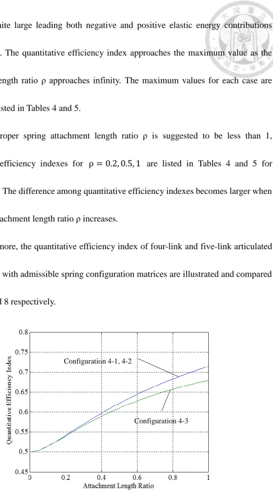
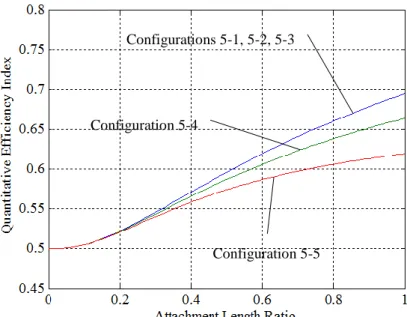
Fig. 7. Quantitative efficiency index of four-link articulated manipulators ... 49

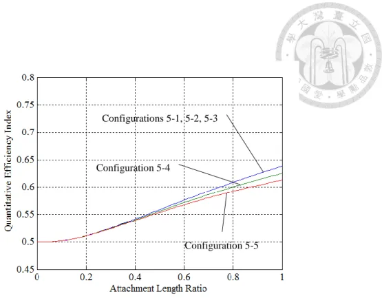
Fig. 8. Quantitative efficiency index of five-link articulated manipulators ... 50

Fig. 9. Quantitative efficiency index of five-link articulated manipulators with descending link mass ... 56

(8)

Chapter 1 Introduction

1.1 Background

Apparatuses or manipulators tend to move to the location with lowest gravitational

potential energy in gravitational field. It is necessary to neutralize the gravitational effects

on the mechanisms in many cases. Statically balanced articulated manipulators are

mechanisms capable of self-balancing the gravitational effects caused by weight of the

system itself within the workspace. Hence, statically balanced mechanisms are efficient

and easily controlled for no actuating force is required to sustain the system weight.

Technology and new system designs for static balance have been developed in recent

decades [1], and a wide range of applications have been proposed, such as lamps [2],

camera supports [3], surgical light apparatus [4,5], orthoses, rehabilitation devices for

supporting or training [6-9], statically balanced manipulators and robots [10-13], as

shown in Fig. 1.

(9)

(a) (b) (c)

(d) (e)

Fig. 1. Applications for static balance: (a) the angle-poised lamp [2]; (b) the surgical light apparatus [5];

(c) the camera support [3]; (d) the arm supporting device [8]; (e) the lower limb orthosis [6]

Static balance can be achieved by numerous methods such as the joint friction

method, the counterweight method, and the spring method. The counterweight method

requires additional masses to balance the system and may reduce the strength of the

system when the total mass of the system increases [14,15]. The joint friction method

(10)

failure of the system may occur as the joint friction decays. The spring method is therefore

considered the most favorable method among numerous methods proposed to achieve

statically balanced condition for the reason that the elastic potential energy requires only

little additional inertia to neutralize the change in gravitational potential energy induced

by the displacement of the manipulators.

1.2 Overview of related works

The concept to satisfy the statically balanced condition is to keep the total

conservative energy constant. That is to say, the gravitational potential energy U_G and

the elastic potential energy U_E have to compensate the change of each other within the

entire workspace as represented in Eq. (1) where U_Total indicates the total potential

energy.

Total G E

U U U constant (1)

One spring balancing method, as illustrated in Fig. 2 was to install springs with

parallelogram auxiliary mechanisms which delivered the vertical vectors. With the help

of vertical vectors, each link with a parallelogram mechanism on it was independently

balanced by a single spring, and the total potential energy for an n-link manipulator was

kept unchanged [16,17]. Auxiliary parallelogram mechanisms were applied in another

(11)

spring balancing method to form a pantograph shape to locate the mass center as shown

in Fig. 3. Springs were attached to the mass centers to keep the total potential energy

balanced [18-20]. However, methods with auxiliary linkages have some disadvantages,

such as additional inertia and interference caused by auxiliary linkages.

Fig. 2. Spring balancing method with auxiliary linkages to deliver the vertical vectors [16]

Fig. 3. Spring balancing method with auxiliary linkages to locate the mass center [19]

(12)

By adding ground-attached springs to each link of an n-link manipulator, net force

on each link could be reduced to the form of a virtual spring attached to ground. As shown

in Fig. 4, The manipulator were iteratively balanced without auxiliary linkages [21,22].

However, too many ground-attached springs must be installed, which causes problems

such as installation difficulty of springs and interference in workspace.

Fig. 4. Direct spring balancing method by iteratively compensating gravitational effects [22]

Another spring balancing method was the stiffness block matrix approach [23-25].

Gravitational potential energy and elastic potential energy was transformed into the

matrix form and arranged as the gravitational stiffness block matrix [𝐆_𝐮𝐯] and the elastic

stiffness block matrix [𝐊_𝐮𝐯^𝐢𝐤]. The concept of conservation in Eq. (1) were proved to be

equal to that all off-diagonal entries of the summation of the gravitational and elastic

(13)

stiffness block matrix were zero [23,24], represented as Eq. (2) where [𝐓_𝐮𝐯] indicated

the total stiffness block matrix.

N diagonal

     

^T^uv ^G^uv



^K^ik^uv ⁽²⁾

Considering the properties of stiffness block matrices, admissible spring

configurations were derived under objectives of minimum number of springs and

minimum span over number of springs [25].

1.3 Motivation and preview

Based on the stiffness block matrix approach, spring attachment angles were

predetermined and discussed before the discussion about criteria of admissible spring

configurations in previous study [25]. However, previous research focused on the location

and configuration of installed springs, valuable insight from the determination of spring

attachment angles for understanding the function and efficiency of elastic energy was not

well described. The properties of stiffness block matrix can be further discussed to

understand the energy efficiency of statically spring-balanced articulated manipulators.

In this study, the spring installation configurations such as the spring attachment

angles and direction properties of elastic energy contributions are discussed based on the

(14)

Rules for determination of spring installation configurations are elaborated; therefore, the

spring attachment angles and direction properties of elastic energy contributions can be

found for articulated manipulators with different spring configuration matrices. Elastic

energy contributions are therefore identified to be positive contributions or negative

contributions by their direction properties. Elastic energy contributions providing effects

aligned with gravity are redundant for static balance and regarded as negative

contributions. Elastic energy contributions counteracting against gravity and redundant

elastic effects are regarded as positive contributions. A qualitative efficiency index is

proposed as the number ratio of positive elastic energy contributions to total elastic energy

contributions. Furthermore, in the case that the magnitudes of gravitational energy

contributions are taken into consideration, a quantitative efficiency index is proposed as

the magnitude ratio of positive elastic energy contributions to total elastic energy

contributions. Energy efficiency of an n-link statically spring-balanced articulated

manipulators can be assessed according to the proposed efficiency indexes. Comparisons

among four-link and five-link statically balanced articulated manipulators with different

admissible spring configuration matrices are illustrated respectively. A design example is

demonstrated to highlight the practical uses of the efficiency indexes. The energy

efficiency of statically spring-balanced articulated manipulators can be assessed and

(15)

compared during the design processes to help the designer obtained the articulated

manipulator design with minimum energy wastes without trails and errors.

(16)

Chapter 2 Stiffness block matrix representation

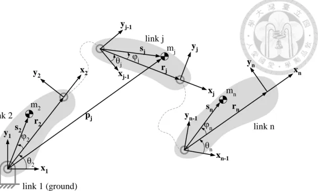
2.1 Gravitational stiffness block matrix

On the basis of Denavit-Hartenberg representation [26], the coordinate system of the

n-link planar articulated manipulator is constructed as shown in Fig. 5. The Cartesian

planar coordinate system is applied on each link. Unit axes x_𝐣 and y_𝐣 are orthonormal

vectors and axis x_𝐣 is aligned on link vector r_𝐣. Each succeeding coordinate system with

respect to its preceding coordinate system can be represented by a rotation matrix 𝐑(θ_j)

[25]. θ_j is the joint angle from the (j − 1)^th coordinate to the j^th coordinate frame.

Moreover, θ_ik is defined as the relative angle from the i^th coordinate frame to the k^th

coordinate frame.

(17)

Fig. 5. Coordinate system of an n-link articulated manipulator

Referring to the n-link articulated manipulator as shown in Fig. 5, the position vector

of mass center of link j denoted by 𝐩_𝐣 is expressed as Eq. (3):

j-1

w=2

= +



j j w

p s r (3)

where 𝐫_𝐰 is the link vector of link w, and 𝐬_𝐣 is the vector from the joint of link j to the

mass center of link j. 𝐫_𝟏 is defined to be equal to 𝐱_𝟏 to keep the symbol consistency in

the following derivations. By expressing each vector as the form of a transformation

matrix times a direction vector [25], the gravitational potential energy denoted by U_G is

derived as Eq. (4):

link 1 (ground) link 2

link j

link n

x₁

x₂ x_j-1

x_j

x_n-1

x_n

y₁

y₂

y_j-1

y_j

y_n-1

y_n

θ₂

θ_j

θ_n φ_n φ_j

s₂

s_j

s_n r₂

r_j

r_n m₂

m_j

m_n p_j

φ₂

(18)

n

G j

j=2

U = -



m ^{g p}^T ^j ⁽⁴⁾

where m_j represents the mass of link j, and g represents the gravitational acceleration

vector. The gravitational potential energy in Eq. (4) can be arranged as the form of

stiffness block matrix representation [23,25], as shown in Eq. (5):

T

G

U 1 2

   

   

 

     

   

   

1 1

2 2

uv

j j

n n

r r

r G r

r r

(5)

where [𝐆_𝐮𝐯] is named the gravitational stiffness block matrix [23,25]. The terms 𝐆_𝐮𝐯

in the gravitational stiffness block matrix are named the gravitational energy components,

where subscribes indicating the term is located in the u^th row of v^th column. Values of

gravitational energy components are expressed as Eq. (6):

 

v ^v

 

v ⁿ w w=v+1 v

g 270 - m s - m for u = 1, v = 2, 3, ..., n r

0 for u 1

  

 

  

   

 





T uv

R R I

G (6)

where R represents the rotation matrix, and I is the 2 × 2 identity matrix. The gravitational stiffness block matrix [𝐆_𝐮𝐯] is expressed as a symmetric matrix in which

(19)

only upper triangular matrix is considered [23,25], the distribution of gravitational

stiffness block matrix is shown in Eq. (7):

0

0 0

0

 

 

    

 

 

 

12 1v 1n

uv

G G G

G (7)

2.2 Property of gravitational stiffness block matrix

Each non-zero gravitational energy component 𝐆_𝟏𝐯 represents the gravitational

energy contribution that acts between ground and link v. Thus, non-zero gravitational

energy components are located only in the first row of the gravitational stiffness block

matrix as expressed in Eq. (7).

Because energy components are mathematically representing planar vector space,

we can rearrange and divide each gravitational energy component into a direction and a

magnitude as expressed in Eq. (8):

     

mag dir for v = 2, 3, ..., n

1v  1v 1v

G G R G (8)

(20)

where dir(𝐆_𝟏𝐯) is the direction and mag(𝐆_𝟏𝐯) is the magnitude of the gravitational

energy component 𝐆_𝟏𝐯. Moreover, the direction and magnitude can be expressed as Eqs.

(9a) and (9b):

   

 

v

v v

v

n v

v v w

w=v+1 v

v

m s sin φ

dir arctan r 270

m s cos φ + m

r φ' 270

 

 

  

 

 

  

1v



G (9a)

     

1

2 n 2 2

v v

v v v v w

w=v+1

v v

s s

mag g m sin φ + m cos φ + m

r r

    

 

   



 

G1v (9b)

The directions of gravitational energy components are the gravitational direction

270° plus an arctangent angle denoted as φ’_v as represented in Eq. (9a). In the case that

the mass center deflection angle φ_v is not equal to zero, the angle φ’_v will not be equal

to zero correspondingly. To be more specifically, the range of φ’_v can be discussed

according to some basic assumptions to obtain a general understanding. If all magnitudes of mass center deflection angles |φ_v| are not greater than 45°, all mass m_v are equal

to each other, and all mass center length ratio ^s_r^v

v are not greater than 0.5, the angle ranges of all φ’_v are determined to be between −22.5° and 22.5°. Since the angle ranges of φ’_v are not considerable in magnitude, it is found that the directions of all gravitational

energy components dir(𝐆_𝟏𝐯) are approximately 270°. On the other hand, the direction

(21)

of gravitational energy component dir(𝐆_𝟏𝐯) becomes far from 270° only when the link

shape is extremely strange, designed deliberately to make φ’_v considerably great in

magnitude.

In this paper, all mass center deflection angles φ_v are assumed to be zero. In other

words, all mass centers of links are assumed to be exactly on the line through the joints

of links. Under the zero φ_v assumption, the direction and magnitude of each

gravitational energy component can be simplified as Eqs. (10a) and (10b):

 

dir G_1v 270 (10a)

 

v ^v ⁿ w

w=v+1 v

mag g m s + m

r

 

  







G1v (10b)

The direction of every gravitational energy component dir(𝐆_𝟏𝐯) is exactly 270°,

as expressed in Eq. (10a), making the discussion in the following sections more clearly

to understand. However, the findings in this study are also valid for the cases with

reasonable mass center deflection angle φ_v.

The mass center is approximately located in the centroid of each link so that the mass center length ratio ^s_r^v

v is generally suggested to be less than 1 intuitively. Under the circumstances, the magnitudes of gravitational energy components mag(𝐆_𝟏𝐯) are

distinct to each other in a descending order from v = 2 to v = n according to Eq. (9b).

(22)

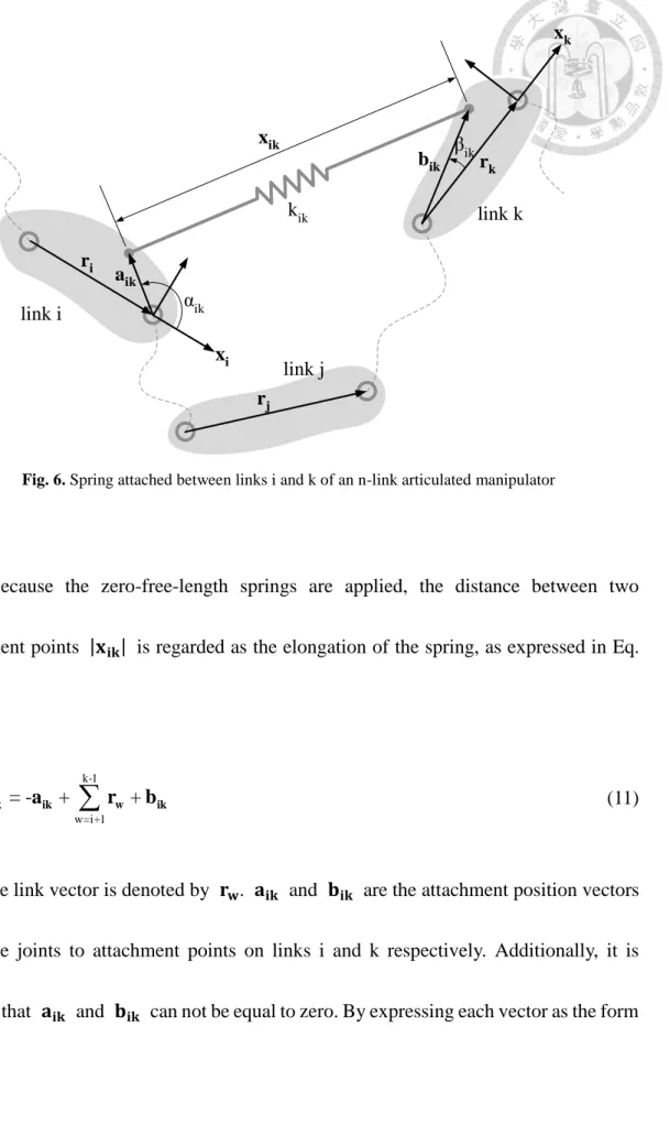
2.3 Elastic stiffness block matrix

For a statically balanced articulated manipulator, a spring configuration matrix [S_uv], an n × n matrix, is defined to represent the configuration of installed springs

[24,25]. Only one spring at most is allowed to be attached between two links. The non-

zero element of S_uv = # which lies in the u^th row of v^th column stands for a spring

attached between links u and v. Only the upper triangular spring configuration matrix is

considered because of the symmetry and redundancy [24,25].

As illustrated in Fig. 6, a spring with spring constant k_ik attached between links i

and k of an n-link articulated manipulator is denoted by S_ik= # in the spring

configuration matrix. Furthermore, since link i is the proximal attached link and link k is

the distal attached link, i is defined to be less than k.

(23)

Fig. 6. Spring attached between links i and k of an n-link articulated manipulator

Because the zero-free-length springs are applied, the distance between two attachment points |𝐱_𝐢𝐤| is regarded as the elongation of the spring, as expressed in Eq.

(11):

k-1

w=i+1

= - +



+

ik ik w ik

x a r b (11)

The link vector is denoted by 𝐫_𝐰. 𝐚_𝐢𝐤 and 𝐛_𝐢𝐤 are the attachment position vectors

from the joints to attachment points on links i and k respectively. Additionally, it is

defined that 𝐚_𝐢𝐤 and 𝐛_𝐢𝐤 can not be equal to zero. By expressing each vector as the form link i

link j

link k

r_j r_i

r_k

x_k

b_ik β_ik x_ik

k_ik

x_i α_ik a_ik

(24)

of a transformation matrix times a direction vector [25], the elastic potential energy from

spring S_ik is denoted by U_E^ik and derived as Eq. (12):

ik

E ik

U = 1k 2

T ik ik

x x (12)

Notice that U_E shown in Eq. (1) denotes the elastic potential energy of the whole

system, while U_E^ik represents the elastic potential energy from spring S_ik. The elastic

potential energy in Eq. (12) can be arranged as the form of stiffness block matrix

representation as shown in Eq. (13) [23,25]:

T

ik

UE 1 2

   

   

 

     

   

   

1 1

2 2

ik uv

j j

n n

r r

r K r

r r

(13)

where [𝐊_𝐮𝐯^𝐢𝐤] is named the elastic stiffness block matrix [23,25]. The terms 𝐊_𝐮𝐯^𝐢𝐤 in the

elastic stiffness block matrix are named the elastic energy components [23,25]. The

superscripts indicate that the term is induced by the spring attached between links i and

k, and the subscripts indicate that the term is located in the u^th row of v^th column.

Diagonal elastic energy components 𝐊_𝐮𝐯^𝐢𝐤 with u = v are expressed as Eqs. (14a-

c):

(25)

2 ik ik

i 2 ik ik

k

ik

k ar u = v = i (a)

k b u = v = k (b)

r

u = v = i+ 1, , k- 1 (c) k

  

  

  

  

   

 



ik uv

I

K I

I

(14)

Off-diagonal elastic energy components 𝐊_𝐮𝐯^𝐢𝐤 with u ≠ v are expressed as Eqs.

(15a-d):

 

ik

ik ik

i ik

ik ik

k ik ik

ik ik ik

i k

ik

a u i; v i 1, , k - 1 (a)

k 180 -

r

b u i 1, , k - 1; v k (b)

k r

a b

u i; v k (c)

k 180 -

r r

u, v i 1, , k - 1 (d)

k 0

       



      

 

       



     



ik p

ik ik D

uv

ik L

ik S

R K

K

R K

(15)

where α_ik and β_ik are the proximal and distal attachment angles respectively; ^a_r^ik

i and

b_ik

r_k are the proximal and distal attachment length ratios respectively.

2.4 Property of elastic stiffness block matrix

Energy components are mathematically representing planar vector space, and can

therefore be divided into a direction and a magnitude. Notice that the representation of

elastic energy components expressed in Eqs. (14a-c) and (15a-d) are already divided into

a direction and a magnitude as the form shown in Eq. (16):

(26)

     

mag dir



ik ik ik

uv uv uv

K K R K (16)

Each non-zero elastic energy component 𝐊_𝐮𝐯^𝐢𝐤 stands for the elastic energy

contribution that acts between links u and v caused by the spring attached between links i and k (S_ik).

The change of the relative angle θ_uv causes an energy variation of 𝐫_𝐮^𝐓𝐊_𝐮𝐯^𝐢𝐤𝐫_𝐯.

Therefore, the elastic energy contribution from the diagonal elastic energy component 𝐊_𝐮𝐯^𝐢𝐤 with u = v does not vary when the relative position of links change, since the

relative angle θ_uv with u = v is always zero. That is to say, the diagonal energy

components in Eq. (14a-c) are irrelevant to statically balanced condition; therefore, only

off-diagonal energy components are considered during the discussion about static balance.

The total number of off-diagonal elastic energy components for the spring attached

between links i and k is determined to be (k−i+1)(k−i)

2 , and is regarded as the number of total elastic energy contributions. The number of total elastic energy contributions are

listed in Tables 2 and 3 respectively for the four-link and five-link articulated

manipulators with the spring configuration matrices assessed in this study. Intuitively, the

number of total elastic energy contributions should be as little as possible for the reason

that springs with less number of total contributions are less complicated in the form of

energy performance, leading the possible energy waste less likely to occur. Thus, the

(27)

examples demonstrated in this study shown in Tables 2 to 5 are ordered ascendingly by

the number of total elastic energy contributions as a brief guess that the less the number

of total contributions is, the more efficient the articulated manipulator is.

Off-diagonal elastic energy components are denoted by the symbol 𝐊_𝐮𝐯^𝐢𝐤 with

different subscripts according to the locations. However, only four distinct values exist

among them. It is confusing when symbols with different subscripts are representing the

same value. Therefore, the denotations of off-diagonal elastic energy components are

further simplified as 𝐊_𝐏^𝐢𝐤, 𝐊_𝐃^𝐢𝐤, 𝐊_𝐋^𝐢𝐤, 𝐊_𝐒^𝐢𝐤.

Elastic energy components dominated by the proximal installation configurations

a_ik

r_i and α_ik of the spring are called the proximal elastic energy components, denoted as 𝐊_𝐏^𝐢𝐤 shown in Eq. (15a). All the proximal elastic energy components 𝐊_𝐏^𝐢𝐤 are located in

the i^th row. Elastic energy components dominated by the distal installation

configurations ^b_r^ik

k and β_ik of the spring are called the distal elastic energy components, denoted as 𝐊_𝐃^𝐢𝐤 shown in Eq. (15b). All the distal elastic energy components 𝐊_𝐃^𝐢𝐤 are

located in the k^th column. Elastic energy component dominated by both proximal and

distal installation configurations ^a_r^ik

i, α_ik, ^b_r^ik

k and β_ik of the spring is called the leading elastic energy component, denoted as 𝐊_𝐋^𝐢𝐤 shown in Eq. (15c). The leading elastic energy

𝐢𝐤 th th

(28)

with value k_ik𝐑(0°) are called the side effect elastic energy components, denoted as 𝐊_𝐒^𝐢𝐤 expressed in Eq. (15d). All the side effect elastic energy components 𝐊_𝐒^𝐢𝐤 are

located in the (i + 1)^th to (k − 1)^th rows of (i + 1)^th to (k − 1)^th columns,

directions of which are all 0°. Side effect elastic energy components 𝐊_𝐒^𝐢𝐤 are considered

troublesome and needed to be balanced by other springs.

The distribution of elastic stiffness matrix [𝐊_𝐮𝐯^𝐢𝐤] is expressed in Eq. (17):

0 0 0 0 0 0 0

0 0 0 0 0 0

 

 

  

   

 

 

ik ik ik ik ik

uv P P P L

ik ik ik ik

uv S S D

ik ik ik ik

uv uv S D

ik ik

uv D

ik uv

K K K K K

K K K K

K K

K

(17)

Only the upper triangular matrix is considered since the 𝐊_𝐯𝐮^𝐢𝐤 is the transpose of 𝐊_𝐮𝐯^𝐢𝐤 [23,25].

(29)

Chapter 3 Spring installation configurations

3.1 Examination of energy counteraction from vector perspective

For four-link and five-link articulated manipulators, admissible spring configuration

matrices under the objective of minimum span over number of springs [25] are listed in

Tables 2 and 3 respectively. Starting from an admissible spring configuration matrix, the

energy contributions in the total stiffness block matrix of a specific spring configuration

can be presented according to the definition of gravitational and elastic stiffness block

matrix shown in Eqs. (7) and (17).

For example, starting from the spring configuration matrix 5-4 shown in Table 3,

following the definition of gravitational and elastic stiffness block matrix shown in Eqs.

(7) and (17), the energy contributions in the total stiffness block matrix can be expressed

as shown below in Eq. (18):

  N 

   

 

 

 

 

 

 ^ik

uv uv

15 14 12 15 14 15 14 15

12 P P L 13 P P 14 P L 15 L

15 25 14 23 15 25 14 15 25

S P S L S P D D L

15 25 14 15 25

S S D D D

15 25

D D

G K

* G + K + K + K G + K + K G + K + K G + K

* K + K + K + K K + K + K K + K

* K + K + K K + K

* K + K

*

(18)

(30)

Once the distribution of the total stiffness block matrix is acquired, equations derived

from the entries of total stiffness block matrix can be obtained according to the fact that

summation of energy components in the same entry equal to zero.

Energy components are 2 × 2 matrices which consist of four terms for each of them,

so the fact that summation of energy components in the same entry equal to zero ought to

provide four linear equations. However, only two out of the four linear equations are

independent because both gravitational and elastic energy components are

mathematically representing planar vector space which consist of only two independent

variables, directions and magnitudes. By dividing each energy component into a direction

and a magnitude as expressed in Eqs. (8) and (16), the general knowledge of vector

operations can be applied throughout the study.

Thus, it is much easier to understand the philosophy of the neutralization among

energy components for static balancing if each energy component is considered as a

vector; while it is more compact to present the whole system in matrix form. By

examination of the total stiffness block matrix, which expresses the counteraction

between gravitational and elastic potential energy, the spring attachment angles are found

to be determined according to some specific rules.

(31)

3.2 Characteristics for determination of spring installation configurations

First of all, only energy components 𝐆_𝟏𝐧 and 𝐊_𝐋^𝟏𝐧 exist in entry 1n for every

admissible spring configuration. Since the sum of 𝐆_𝟏𝐧 and 𝐊_𝐋^𝟏𝐧 is equal to zero to

achieve static balance, 𝐊_𝐋^𝟏𝐧 must have the opposite direction and the equal magnitude

compared with 𝐆_𝟏𝐧. On account of the direction property of gravitational energy

components, rule 1 can be derived as shown in Table 1: for the spring attached between ground and end link (S_1n), the attachment angle β_1n− α_1n must be 270°.

If no spring is attached between link 3 and end link, Eqs. (19a) and (19b) can be

obtained considering the neutralization within entry 2n and entry 3n. Therefore, for the spring attached between link 2 and end link (S_2n), 𝐊_𝐋^𝟐𝐧 must be equal to 𝐊_𝐃^𝟐𝐧 to keep

both Eqs. (19a) and (19b) satisfied; hence, the attachment angle α_2n must be 180° and

attachment length ratios ^a_r²ⁿ

2 must be 1 to keep 𝐊_𝐋^𝟐𝐧 and 𝐊_𝐃^𝟐𝐧 equal. Therefore, rule 2 can be obtained as shown in Table 1.

 0

1n 2n

D L

K K (19a)

 0

1n 2n

D D

K K (19b)

General equations based on the neutralization within entries 1(k+1), 1k and 1(k-1)

(32)

derived by subtracting Eq. (20a) from Eq. (20b). For a spring attached between ground and link k (S_1k), if no spring or only spring whose direction of energy components

𝐊_𝐏^{𝟏(𝐤+𝟏)}− 𝐊_𝐋^{𝟏(𝐤+𝟏)} equals to 270° is attached between ground and link (k+1),

considering Eq. (20d) on account of the direction property and magnitude property of

gravitational energy components, it is required that the direction of energy component 𝐊_𝐋^𝟏𝐤 must be 90° to keep entry 1k balanced because the direction of the summation of

all the other energy components in Eq. (20d) is 270°. Therefore, the attachment angle β_1k− α_1k for S_1k must be 270°. Rule 3 shown in Table 1 is obtained accordingly.

n

v=k+2





^1v  ^1(k+1) 0

1(k+1) P L

G K K (20a)

n

v=k+1





^1v  ^1k 0

1k P L

G K K (20b)

n

v=k





^1v  ^1(k-1) 0

1(k-1) P L

G K K (20c)



G1k ^G1(k+1)



^



K^1(k+1)P ^K^1(k+1)L



^K^1kL ^⁰ (20d)



^G^1(k-1) ^^G^1k



^



^K^1k^P ^^K^1k^L



^^K^1(k-1)^L ^⁰ ^(20e)

Eq. (20e) can be derived by subtracting Eq. (20b) from Eq. (20c). For a spring attached between ground and link k (S_1k), if no spring or only spring with attachment

(33)

angle β_1(k−1)− α_1(k−1) = 90° is attached between ground and link (k-1), considering

Eq. (20e) on account of the direction property and magnitude property of gravitational

energy components, the direction of energy components 𝐊_𝐏^𝟏𝐤− 𝐊_𝐋^𝟏𝐤 must be 90° to

keep entry 1k balanced because the direction of the summation of all the other energy

components in Eq. (20e) is 270°. Therefore, rule 4 can be obtained as shown in Table 1.

It is noticed that rule 4 does not provide direct constraints on spring attachment angles

and only gives a relationship between elastic energy components. Nevertheless this

relationship is useful for the determination of spring attachment angles, if other

constraints are considered at the same time. For example, if rules 3 and 4 are applied to a

spring S_1k at the same time, the attachment angle β_1k− α_1k must be 270° according

to rule 3; the attachment angle α_1k must be 90° according to the constraints provided

by both rules 3 and 4. Another example is that if rules 4 and 5 are applied to a spring S_1k

at the same time, the attachment angle β_1k must be 180° according to rule 5; the

attachment angle α_1k must be 90° according to the constraints provided by both rules

4 and 5.

Considering the neutralization within an arbitrary entry ik with i ≠ 1 and k ≠ n, all springs attached between links u and v (S_uv) for 1 ≤ u ≤ i − 1 and k + 1 ≤ v ≤ n

(34)

elastic energy components are inevitably to be 0° as mentioned in the aforementioned

section shown in Eq. (15d). Hence, to neutralize these 0° direction energy components

in entry ik, the direction of the summation of all the following elastic energy components

contributed to entry ik must be 180°: the leading elastic energy components from springs

attached between links i and k, the proximal elastic energy components from springs

attached between links i and v for each k + 1 ≤ v ≤ n, and the distal elastic energy

components from springs attached between links u and k for each 1 ≤ u ≤ i − 1. Thus,

some of the spring attachment angles can be determined in order to neutralize the 0°

direction energy components caused by other springs.

A spring attached between links i and k (S_ik) with k − i ≥ 2 must contribute its

distal elastic energy component as a 180° direction energy component to balance the

entry (i+1)k, if no spring or only springs with attachment angle β_uk = 0° are attached

between links u and k for each 1 ≤ u ≤ i − 1, and if no spring or only springs with

attachment angle α_(i+1)v = 180° are attached between links (i+1) and v for each k + 1 ≤ v ≤ n, and if no spring or only spring with attachment angle β_(i+1)k− α_(i+1)k =

180° is attached between links (i+1) and k. Therefore, the attachment angle β_ik for S_ik

must be 180° and rule 5 is obtained in Table 1 accordingly.

(35)

A spring attached between links i and k (S_ik) with k − i ≥ 2 and i ≠ 1 must

contribute its proximal elastic energy component as a 180° direction energy component

to balance the entry i(k-1), if no spring or only springs with attachment angle α_iv= 180°

are attached between links i and v for each k + 1 ≤ v ≤ n, and if no spring or only

springs with attachment angle β_u(k−1) = 0° are attached between links u and (k-1) for

each 1 ≤ u ≤ i − 1, and if no spring or only spring with attachment angle β_i(k−1)− α_i(k−1) = 180° is attached between links i and (k-1). Hence, the attachment angle α_ik

for S_ik must be 0° as rule 6 describes shown in Table 1.

A spring attached between links i and k (S_ik) with i ≠ 1 must contribute its leading

elastic energy component as a 180° direction energy component to balance the entry ik,

if no spring or only springs with attachment angle α_iv= 180° are attached between links

i and v for each k + 1 ≤ v ≤ n, and if no spring or only springs with attachment angle β_uk = 0° are attached between links u and k for each 1 ≤ u ≤ i − 1 .Thus, the

attachment angle β_ik− α_ik for S_ik must be 0°, and rule 7 can be obtained accordingly

as described in Table 1.

(36)

Table 1

Rules for determination of spring attachment angles from admissible spring configuration matrices

3.3 Determination of spring attachment angles

The determination of spring attachment angles following the rules described in the

aforementioned section is demonstrated in this section.

First of all, rule 1 is always valid for any admissible spring configuration, because the spring attached between ground and end link (S_1n) is the only spring able to neutralize

the gravitational energy contribution in entry 1n. It is determined that the attachment

angle β_1n− α_1n is equal to 270° according to rule 1. Then, based on the requirement

described in rule 2, if no spring is attached between link 3 and end link, for the spring attached between link 2 and end link (S_2n), it is determined that the attachment angle α_2n

is equal to 180° according to rule 2. Take the spring configuration matrix 5-4 as an

example, it is determined that the attachment angle β₁₅− α₁₅ is equal to 270° for S₁₅

(37)

according to rule 1, and that the attachment angle α₂₅ is equal to 180° for S₂₅

according to rule 2.

Based on rule 5, for each spring attached between ground and link k (S_1k) where

2 ≤ k ≤ n, if no spring attached between links 2 and v for k ≤ v ≤ n contributes an

energy component with 180° direction to entry 2k, the sufficient condition of rule 5 is

satisfied for the spring S_1k. Therefore, the spring S_1k is in charge of contributing an

energy component with 180° direction to entry 2k and the attachment angle β_1k is

determined to be 180° according to rule 5. Take the spring configuration matrix 5-4 as

an example, because no spring is attached between links 2 and 4 and the attachment angle α₂₅ is 180° for the spring attached between links 2 and 5 according to rule 2. It is

determined that the attachment angle β₁₄ is equal to 180° for S₁₄ according to rule 5.

In accordance with rule 3, if S_1k = # and S_1(k+1) = 0 in the first row of spring

configuration matrix, it is determined that the attachment angle β_1k− α_1k is equal to 270° for S_1k. After the attachment angles of spring S_1k is determined, in the case that

S_1(k−1) = #, it is determined that the attachment angle β_1(k−1)− α_1(k−1) is equal to

270° for S_1(k−1) if the direction of energy components 𝐊_𝐏^𝟏𝐤− 𝐊_𝐋^𝟏𝐤 is equal to 270°

for S_1k according to rule 3. Likewise, in the case that S_1(k−2)= #, S_1(k−3) = #, and so

(38)

according to rule 3. Take the spring configuration matrix 5-4 as an example, because no

spring is attached between ground and link 3, it is determined that attachment angle β₁₂− α₁₂ is equal to 270° for S₁₂ according to rule 3.

On the basis of rule 4, if S_1k = # and S_1(k−1) = 0 in the first row of spring

configuration matrix, it is determined that the direction of energy components 𝐊_𝐏^𝟏𝐤− 𝐊_𝐋^𝟏𝐤 must be 90° for S_1k. After the attachment angles of S_1k is determined, in the case

that S_1(k+1) = #, it is determined that the direction of energy components 𝐊_𝐏^{𝟏(𝐤+𝟏)}− 𝐊_𝐋^{𝟏(𝐤+𝟏)} must be 90° for S_1(k+1) if the attachment angle β_1k− α_1k is equal to 90°

for S_1k according to rule 4. Likewise, in the case that S_1(k+2)= #, S_1(k+3) = #, and so

on, attachment angles can be determined iteratively if the requirements are achieved

according to rule 4. Take the spring configuration matrix 5-4 as an example, because no

spring is attached between ground and link 3, it is determined that the direction of energy

components 𝐊_𝐏^𝟏𝟒− 𝐊_𝐋^𝟏𝟒 must be 90° for S₁₄ according to rule 4. Combined with the

fact that the attachment angle β₁₄ is equal to 180° for S₁₄ according to rule 5, the

attachment angle α₁₄ is determined to be 90° accordingly. Iteratively, it is determined

that the direction of energy components 𝐊_𝐏^𝟏𝟓− 𝐊_𝐋^𝟏𝟓 must be 90° for S₁₅ according to

rule 4 because the attachment angle β₁₄− α₁₄ is equal to 90° for S₁₄. Combined with

(39)

the fact that the attachment angle β₁₅− α₁₅ is equal to 270° for S₁₅ according to rule

1, the attachment angle α₁₅ is determined to be 90° accordingly.

To ensure that the neutralization is accomplished for every entry in the non-first rows

of the total stiffness block matrix, at least one energy component with 180° direction

must be contributed to each entry in the non-first rows. Hence, for every the non-zero

element in the spring configuration matrix, the requirements according to rules 5, 6 and

7 have to be examined, starting from springs with larger span over number k − i to those

with smaller span over number.

If a spring attached between links i and k (S_ik) is the only spring able to contribute

an energy component with 180° direction to entry (i+1)k, it is determined that the

attachment angle β_ik is equal to 180° for S_ik according to rule 5. If a spring attached between links i and k (S_ik) is the only spring able to contribute an energy component with

180° direction to entry i(k-1), it is determined that the attachment angle α_ik is equal to

0° for S_ik according to rule 6. If a spring attached between links i and k (S_ik) is the only

spring able to contribute an energy component with 180° direction to entry ik, it is

determined that the attachment angle β_ik− α_ik is equal to 0° for S_ik according to rule

7. Take the spring configuration matrix 5-4 as an example, it is determined that the

β 180° for S

(40)

attachment angle β₂₅− α₂₅ has to be 0° for S₂₅ according to rule 7, and that the

attachment angle β₂₃− α₂₃ has to be 0° for S₂₃ according to rule 7.

(41)

Chapter 4 Qualitative efficiency index

4.1 Identification of energy contributions by spring installation configurations

Attachment angles of installed springs are determined dependent on the spring

configuration matrix. Moreover, for a spring configuration under the objective of

minimum span over number of springs [25], all spring attachment angles must be

determined according to the described rules because the design parameters of springs are

just enough to satisfy the constraint equations derived from the total stiffness block matrix.

Therefore, the spring attachment angles are not arbitrary choices but determined values

when the spring configuration matrix is selected. That is to say, we can select an

admissible spring configuration matrix and determine the attachment angles of installed

springs by examining the counteraction between gravitational and elastic potential energy

expressed in the total stiffness block matrix.

The direction properties of elastic energy components are also determined

simultaneously. For the elastic energy contributions in the first row, contributions with 270° direction are providing effects aligned with gravity and identified as negative

contributions which are harmful for static balance; elastic energy contributions with 90°

(42)

which are beneficial for static balance. For the elastic energy contributions in the non-

first rows, contributions with 0° direction are redundant spring side effects which are

undesired for static balance and identified as negative contributions; elastic energy

contributions with 180° direction are counteracting against spring side effects and

identified as positive contributions.

Take the articulated manipulator with spring configuration matrix 5-4 as the example,

attachment angles of spring S₁₄ are α₁₄= 90° and β₁₄ = 180° as described in Table

3. The direction of the proximal elastic energy component 𝐊_𝐏^𝟏𝟒 is 90° according to Eq.

(15a); therefore, 𝐊_𝐏^𝟏𝟒 is a positive contribution. Likewise, the distal elastic energy

component 𝐊_𝐃^𝟏𝟒 is a positive contribution with 180° direction according to Eq. (15b);

the leading elastic energy component 𝐊_𝐋^𝟏𝟒 is a negative contribution with 270°

direction according to Eq. (15c); the side effect elastic energy component 𝐊_𝐒^𝟏𝟒 is a

negative contribution with 0° direction according to Eq. (15d).

The distribution of total stiffness block matrix can be rearranged as the form

expressed below in Eq. (21) where the positive contributions are placed in the right side

and the negative contributions are placed in the left side.

彈簧靜平衡機構之能量效率分析

國立臺灣大學工學院機械工程學系 碩士論文

Department of Mechanical Engineering College of Engineering

National Taiwan University Master Thesis

彈簧靜平衡機構之能量效率分析 Energy Efficiency Assessment of

Statically Spring-Balanced Articulated Manipulators

楊智涵 Chih-Han Yang

指導教授：陳達仁 博士 Advisor: Dar-Zen Chen, Ph.D.

中華民國 105 年 7 月

July 2016

中文摘要

Abstract

Contents

Chapter 1 Introduction ... 1

Chapter 2 Stiffness block matrix representation ... 9

Chapter 3 Spring installation configurations ... 22

Chapter 4 Qualitative efficiency index ... 34

Chapter 5 Quantitative efficiency index ... 42

Chapter 6 Design example ... 52

Chapter 7 Conclusions ... 58

Reference ... 60

List of Tables

List of Figures

Chapter 1 Introduction



Chapter 2

Stiffness block matrix representation





 

 



     

   

 



     



 

 





 

 

 

 

     

Chapter 3

Spring installation configurations























Chapter 4

Qualitative efficiency index

國立臺灣大學工學院機械工程學系碩士論文

指導教授：陳達仁博士 Advisor: Dar-Zen Chen, Ph.D.