深開挖基地三維幾何配置於連續壁壁體變位之影響

(1)

國立臺灣大學工學院土木工程學系碩士論文

Graduate Institute of Civil Engineering College of Engineering

National Taiwan University Master Thesis

深開挖基地三維幾何配置於連續壁壁體變位之影響 The Effect of Three Dimensional Configurations on the Diaphragm Wall Displacements Due to Deep Excavation

張智博 Chih-Po Chang

指導教授：葛宇甯教授 Advisor: Prof. Louis Ge

中華民國 105 年 6 月

June, 2016

(2)

(3)

誌謝

兩年。

回首這些日子，見到自己緩慢但穩健地走了一段路，甚感欣慰。

感謝指導老師葛宇甯教授，在我和此研究上挹注了許多資源以及心力，並給予足夠的空間選擇研究的方法且不厭其煩地讓我嘗試與修正，使我碩士生涯十分充實。

感謝同窗黃郁惟在報告前總耐心地聽我練習並給予意見，甚至一起討論研究的方法以及盲點。

感謝同窗王棋立提供 BIC 以及 SVM 的應用技術，使我能夠更廣泛地嘗試各種方法進行研究。

感謝女友蕭至妤這幾年來的包容，包容我經常地晚歸，以及常常以作研究為藉口，躲在研究室不回家做家事。

最感謝父母，在我就學期間提供精神以及經濟上的支持，讓我能夠心無旁鶩地埋首於課業及研究中。

最後，還記得國中時的各種荒唐行徑，感謝秦冀萍老師及時拉住我，否則我甚至會選擇不繼續升學。

台大魔甘娜之王，畢業啦!

(4)

(5)

ABSTRACT

Diaphragm walls are often used to resist lateral earth pressure and prevent excess ground settlement and wall movements during excavations. There are several practical methods for diaphragm wall design, based on the assumption of plane strain condition.

This assumption is valid for shallow and wide excavations, with L/He value greater than 6 (L: length of diaphragm wall, He: depth of excavation). Due to limited available space in urban area, lots of excavations are small but deep in Taiwan. Without considering the three dimensional effects, it leads to an over conservative design for the diaphragm wall.

To develop an economical method for diaphragm wall design with consideration of three dimensional effect, the finite element software “Plaxis” was used to examine the maximum wall deflection in various combinations of thickness of wall, average vertical and horizontal spacing of struts, length and width of excavation, and maximum ground water head difference.

From the simulation results, the new system stiffness was proposed. As the current study focuses on the excavations in sand, case histories excavated mainly in the sandy layer were selected to verify the applicability of the proposed system stiffness. It was concluded that the proposed system stiffness can quantify the wall stiffness more precisely with consideration of the three dimensional effects, especially in the condition of high system stiffness.

(6)

摘要

連續壁常見於深開挖工程之擋土系統，用以抵抗側向土壓力並防止開挖工址周圍產生過大的地表沉陷量造成損鄰。目前實務中，連續壁設計方法多建立於平面應變條件之上；然而此條件適於較淺且較廣的開挖工程，即開挖長度(L)與開挖

深度(He)比值高於 6 者。因空間有限，臺灣現今於市區及近郊的深開挖工程多呈小

且深之設計，已不符平面應變條件之假設；倘若不思三向度效應，將導致擋土系統過度設計，所耗成本甚鉅。

為發展考量三向度效應之連續壁設計方法，此研究採用有限元素分析軟體 Plaxis 模擬於砂土中開挖引致的連續壁壁體變形行為，分析三向度幾何因子，如壁體厚度、平均垂直與水平支撐間距、開挖基地之長與寬等，以及外力因子，基地內外最大水頭差，對於連續壁壁體最大變形量所造成的影響。

根據上述之模擬結果，歸納出可考量三向度效應的新系統勁度。因本研究著眼於砂土中開挖的連續壁壁體變形行為，故採用地層主要由砂性土壤組成之案例驗證所提出之系統勁度。

本研究提出之系統勁度於高勁度擋土系統之預測較為準確。

(7)

(8)

LIST OF FIGURES

Fig. 1 1 Flow chart of research methodology ... 3 Fig. 2. 1 Design chart for estimating maximum lateral wall movement in soft to medium clays. (Clough and O'Rourke, 1990) ... 8 Fig. 2. 2 Distribution of soil stress while soil arching occurs. (Evans, 1984) ... 8 Fig. 2. 3 Distribution of soil stress in active and passive arching. (Evans, 1984) ... 9 Fig. 2. 4 Variation of maximum wall displacement with the distance from the corner for constant sizes of complementary wall and various sizes of primary wall. (Ou, et al., 1996) ... 10 Fig. 2. 5 Variation of PSR for maximum wall displacement with the distance from the corner for constant sizes of primary wall and various sizes of complementary wall. (Ou et al., 1996) ... 10 Fig. 2. 6 Relationship between ratio of complementary wall length to primary wall length and distance from corner for various PSR. (Ou et al., 1996)... 11 Fig. 2. 7 Relative stiffness ratio design chart. (Bryson et al., 2012) ... 12 Fig. 2. 8 Comparison of the parametric studies with Clough et al. (1989) design chart.

(Bryson et al., 2012) ... 13 Fig. 3. 1 Cross section of retaining system and soil layers of Case A. ... 24

(11)

Fig. 3. 7 Cross sections of MRT side retaining system in Case B. ... 29

Fig. 3. 8 Cross sections of warehouse district retaining system in Case B. ... 30

Fig. 3. 9 Plane view of Case B. ... 31

Fig. 3. 10 Wall deformations obtained by inclinometers in Case B. ... 32

Fig. 3. 11 Wall deformations obtained by measurements and simulations in Case B. .... 33

Fig. 3. 12 Wall deformations shifted to match Plaxis result. ... 34

Fig. 3. 13 Wall deformations shifted to match TORSA result. ... 35

Fig.4. 1 Diagram of studied factors. ... 47

Fig.4. 2 The mesh density of finite element model. ... 48

Fig.4. 3 The performance of S1 on L and B/L. ... 49

Fig.4. 4 The performance of S1 on Hv and Hh. ... 50

Fig.4. 5 The performance of S1 on D and Hw/He. ... 51

Fig.4. 6 The performance of S1 on He. ... 52

Fig.4. 7 New design charts with S1 versus deformation. ... 53

Fig.4. 8 Design charts of different range of L colored by B/L. ... 54

Fig.4. 9 Design charts of different Hw/He colored by L and B/L. ... 55

Fig.4. 10 Design charts of different Hw/He colored by Hv and Hh. ... 56

Fig.4. 11 Design charts of different Hw/He colored by D. ... 57

Fig.4. 12 New design charts with S2 versus deformation. ... 58

(12)

LIST OF TABLES

Table 2. 1 Summary of three dimensional analyses. (Finno et al., 2007) ... 14

Table 2. 2 Stratum conditions. (Finno et al., 2007) ... 14

Table 2. 3 Hardening soil parameters. (Finno et al., 2007) ... 15

Table 2. 4 Parameters of wall. (Finno et al., 2007) ... 15

Table 2. 5 Summary of three dimensional analyses. (Bryson et al., 2012) ... 16

Table 2. 6 Hardening soil parameters for finite element modeling. (Bryson et al., 2012)17 Table 2. 7 Wall rigidity values of each case. (Bryson et al., 2012) ... 18

Table 3. 1 Soil profile of Case A. ... 36

Table 3. 2 Soil parameters of Case A for Mohr-Coulomb model. ... 37

Table 3. 3 Soil profile of Case B. ... 38

Table 3. 4 Soil parameters of Case B for Mohr-Coulomb model. ... 39

Table 4. 1 Parameters of soil, wall, and struts. ... 59

Table 4. 2 Dimensions of excavations in Group A. ... 60

Table 4. 3 Dimensions of excavations in Group B. ... 61

(13)

(14)

Chapter 1 Introduction

Diaphragm walls are usually used as a part of the retaining system during foundation excavation. Current design specifications in Taiwan are primarily focused on the stabilities of the retaining system, which are based on the force or moment equilibrium at the ultimate state. In a modern city, newly constructed structures and facilities are often adjacent to existing structures, such as neighboring buildings, MRT tunnels and so on. In order to minimize the damage to the neighboring structures, the wall-deformation-controlled deign method is in place, where the finite element method (FEM) is a powerful way to simulate the behavior of the retaining system.

Most FEM simulations are conducted by two dimensional models, with an assumption of plane strain for the excavation. This leads to an overestimation of the diaphragm wall deformations. Thus, it is necessary to examine the three dimensional effect in excavations.

1.1 Motivation

The excavations have become deeper and narrower in Taiwan, especially in Taipei city, for decades. For those small and deep excavations, three dimensional effect plays an important role to wall deformation. However, two dimensional finite element method

(15)

model 4860 three dimensional finite element models for simulating wall deformations for top-down excavations.

Then, 9720 sets of wall deformations (each side of excavation can be considered as 1 set of geometric configuration because the L and B could be interchanged, see details in chapter 4.) were used for regression analyses to propose a new system stiffness for the excavation.

Finally, one of the case histories, which was constructed by top-down method, was used to examine the proposed system stiffness and prediction of the regression formula.

The research methodology can be seen more briefly in Fig.1.1.

1.3 Thesis Outline

There are 5 chapters in this thesis. The introduction, including motivation and research methodology, is given in the chapter 1. Previous work on the three dimensional effect, plane strain ratio and relative system stiffness are reviewed and summarized in chapter 2. In the chapter 3, two case histories are studied and simulated. Chapter 4 discusses the settings of three dimensional finite element models and the results of simulations. The conclusions and recommendations to future work are described in the chapter 5.

(16)

Literature Review Excavation Case Histories in Sandy Soil

4860 Models with Variation of Each Factor

Find Significant Factors Examine Modeling Method

Propose New System Stiffness

Conclusions

(17)

Chapter 2 Literature Review

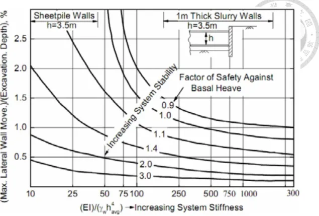
Clough et al. (1989) proposed a chart (Fig. 2.1) for engineers to design the retaining system for excavations. However, this chart is more suitable for soldier piles, sheet piles and the likes, whose wall stiffness is flexible and the excavation depth is shallow, than deep excavations today. Dimension of Excavations becomes smaller but deeper nowadays in Taiwan. The retaining wall system becomes stiffer, where the three dimensional effect would affect the deformation of the diaphragm walls significantly.

Therefore, this chart, or other theories under plane strain assumption, would lead to very conservative designs.

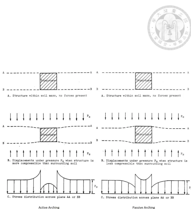
The three dimensional effect could be roughly divided into two mechanisms, the soil arching effect and the corner effect. The definition of soil arching was presented by Terzaghi (1943). It can be applied to excavations. When the diaphragm walls and the adjacent soil mass move against each other, the movement would be resisted by shear stresses. The pressure of the moving soil mass is reduced while the pressure of adjacent rigid soil mass is increased (Fig. 2.2). The soil arching effect can be subdivided into active and passive archings, depending upon the direction of the relative movements, as shown in Fig. 2.3.

Three dimensional effects in deep excavation are contributed by several factors, including excavation depth, height of diaphragm wall, length and width of excavation, horizontal and vertical spacing of struts, and so on. There are mainly two approaches to account for the three dimensional effects, plane strain ratio (PSR) and relative stiffness ratio. They are described in this chapter.

(18)

2.1 Plane Strain Ratio (PSR)

Due to the plane strain assumption that the diaphragm wall deflection in out-of-plane direction should be uniform, the result of two dimensional finite element analysis in deep excavation tends to be too conservative, especially in narrow but deep excavations.

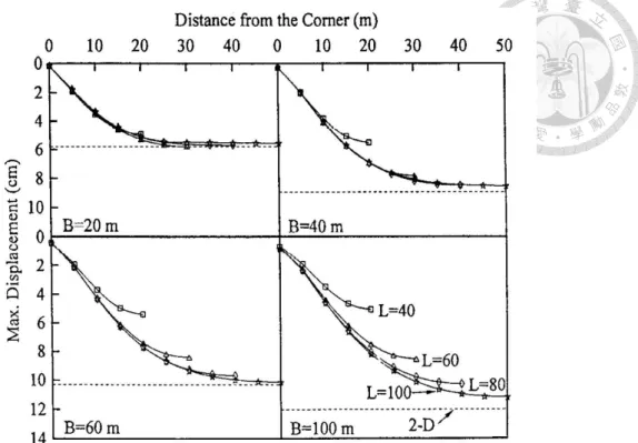
Ou et al. (1996) used two and three dimensional finite element models to simulate the wall deflections in excavations of different distance from the corner, primary wall and complementary wall length.

They defined plane strain ratio (PSR) as the ratio of the maximum wall displacement of a section in the three dimensional analysis to the maximum wall displacement of a section under plane strain condition. From the result shown in Fig. 2.4 and Fig. 2.5, the conclusions were made that the deflections of short primary wall affected by distance to the corner heavily than longer primary wall does, while the longer primary wall is, the larger parts of wall would reach the plane strain condition.

The chart of the length of secondary wall to the length of primary wall ratio versus distance from the corner was proposed (Fig. 2.6). The chart was divided into several zone by different plane strain ratios.

In addition, the convergence study was carried out before the large amount of numerical analyses. They found that the mesh density outside the excavation would be

(19)



 

 























1 05 . 0

1 B

e L

PSR ^H^e

L kC

where C is the factor depending on the factor of safety against basal heaving FSBH:

 



FSBH



C1 0.51.8

And k is the factor depending on the system stiffness S defined by Clough et al. (1989):

S k 10.0001

4 . avg wh S EI



They concluded that when the ratio of the wall length to excavation depth He

L is

greater than 6, the PSR would be very close to 1, indicating that the wall behavior corresponds to plane strain condition. Furthermore, smaller

B

L ratio, stiffer wall

systems and lower factor of safety against basal heaving would produce lower PSR.

However, some other factors affecting the three dimension effects should be taken into consideration, such as struts type, prestress, ground water table and so on.

2.2 Relative system stiffness ratio

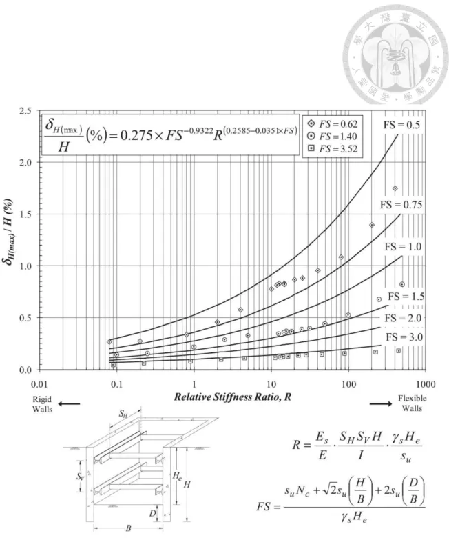
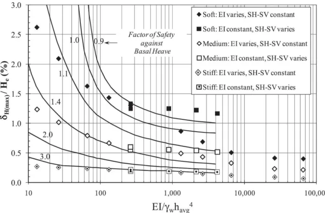
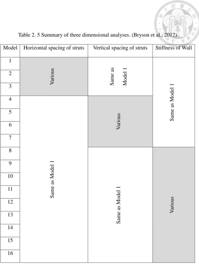
Bryson and Zapata-Medina (2012) used 48 models with different wall stiffness, vertical and horizontal spacing of struts, as listed in Table 2.5 to Table. 2.7, to propose a new system stiffness. The ground water table was assumed to be located at 3 meter below the ground surface and each struts were set 1 meter above excavation surface of last excavation all of the 48 models. They proposed a stiffness ratio called relative system stiffness R:

u e s V H s

s H I

H S S E

R_ E _ _

(20)

where Es is the Young’s modulus of the soil; E is the Young’s modulus of the wall. SH

and SV are average horizontal and vertical spacing of struts respectively. I is moment of inertia per unit length of the wall. H is total height of the wall; He is excavation depth; su

is undrained shear strength of the soil at the bottom of the excavation. The design chart of relative stiffness ratio was shown in Fig. 2.7.

They concluded that the design chart proposed by Clough et al (1989) tends to overestimate the lateral deformation in soft clay and underestimate it for stiff support systems in medium clay (Fig. 2.8).

(21)

Fig. 2. 1 Design chart for estimating maximum lateral wall movement in soft to medium clays. (Clough and O'Rourke, 1990)

Fig. 2. 2 Distribution of soil stress while soil arching occurs. (Evans, 1984)

(22)

Fig. 2. 3 Distribution of soil stress in active and passive arching. (Evans, 1984)

(23)

Fig. 2. 4 Variation of maximum wall displacement with the distance from the corner for constant sizes of complementary wall and various sizes of primary wall.

(Ou, et al., 1996)

Fig. 2. 5 Variation of PSR for maximum wall displacement with the distance from the corner for constant sizes of primary wall and various sizes of

complementary wall. (Ou et al., 1996)

(24)

(25)

Fig. 2. 7 Relative stiffness ratio design chart. (Bryson et al., 2012)

(26)

Fig. 2. 8 Comparison of the parametric studies with Clough et al. (1989) design chart.

(Bryson et al., 2012)

(27)

Table 2. 1 Summary of three dimensional analyses. (Finno et al., 2007)

Stratum He/FSBH L B

A 9.8/1.7, 13.4/1.68, 16.3/1.8 20 20, 40, 80

40 20, 40, 80

80 20, 40, 80, 160^a

160 80^a

B 9.8/1.63, 13.4/1.42, 16.3/1.28 20 20, 40

40 20, 40, 80

80 40, 80

a Analyzed for He equal to 9.8 m only.

Table 2. 2 Stratum conditions. (Finno et al., 2007)

Elevation in Stratum A Elevation in Stratum B

Sand 4.3 ~ -4.8 m 4.3 ~ -4.8 m

Soft Clay -4.8 ~ -12 m -4.8 ~ -14 m

Medium Clay -12 ~ -14 m -14 ~ -24 m

Stiff Clay -14 ~ -24 m N/A

(28)

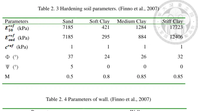
Table 2. 3 Hardening soil parameters. (Finno et al., 2007)

Parameters Sand Soft Clay Medium Clay Stiff Clay

(kPa) 7185 421 1284 17723

(kPa) 7185 295 884 12406

(kPa) 1 1 1 1

Φ (°) 37 24 26 32

Ψ (°) 5 0 0 0

M 0.5 0.8 0.85 0.85

Table 2. 4 Parameters of wall. (Finno et al., 2007)

Parameters Wall

Flexible Medium Stiff

Plane strain parameters

System stiffness, S 32 320 3200

Bending stiffness, EI (MN-m²/m) 50.4 504 5040

Axial stiffness, EA (MN/m) 3427 34270 342700

Thickness (m) 0.42 0.42 0.42

Poisson’s ratio 0 0 0

Three dimensional parameters

Young’s modulus, E1 (MPa) 8160 81600 816000

(29)

Table 2. 5 Summary of three dimensional analyses. (Bryson et al., 2012) Model Horizontal spacing of struts Vertical spacing of struts Stiffness of Wall

1

Various Same as Model 1 Same as Model 1

2 3 4

Same as Model 1 Various

5 6 7 8

Same as Model 1 Various

9 10 11 12 13 14 15 16

(30)

Table 2. 6 Hardening soil parameters for finite element modeling. (Bryson et al., 2012)

Parameters Unit Soft clay Medium clay Stiff clay

kN/m³ 18.1 18.1 20

m/day 0.00015 0.00015 0.00015

m/day 0.00009 0.00009 0.00009

kN/m² 2350 6550 14847

kN/m² 1600 2380 4267

kN/m² 10000 19650 44540

kN/m² 0.05 0.05 0.05

Φ ° 24.1 29 33

Ψ ° 0 0 0

N/A 0.2 0.2 0.2

kN/m² 100 100 100

Power N/A 1.0 1.0 1.0

N/A 0.59 0.55 1.5

kN/m³ 0 0 0

m 0 0 0

N/A 1.00E+15 1.00E+15 1.00E+15

(31)

Table 2. 7 Wall rigidity values of each case. (Bryson et al., 2012)

Model α α*EI (kN-m²/m)

1-7 1 540675

8 0.05 2703.75

9 0.1 54067.5

10 0.25 135168.75

11 0.5 270337.5

12 5 2703375

13 10 5406750

14 25 13516875

15 100 54067500

16 250 135168750

(32)

(33)

Chapter 3 Case Studies

The excavations in sandy soil are seldom studied in those research on the three dimensional effect in excavations. Therefore, the influence of three dimensional effect of excavations in sand are used as the subject of this study

Two case histories of foundation excavations located in Kaohsiung and Taipei, whose soil profiles are mainly consisted of sandy soil, were used as verifications of modeling framework. The results of three dimensional and two dimensional analyses were compared with in situ measurements.

3.1 Case A

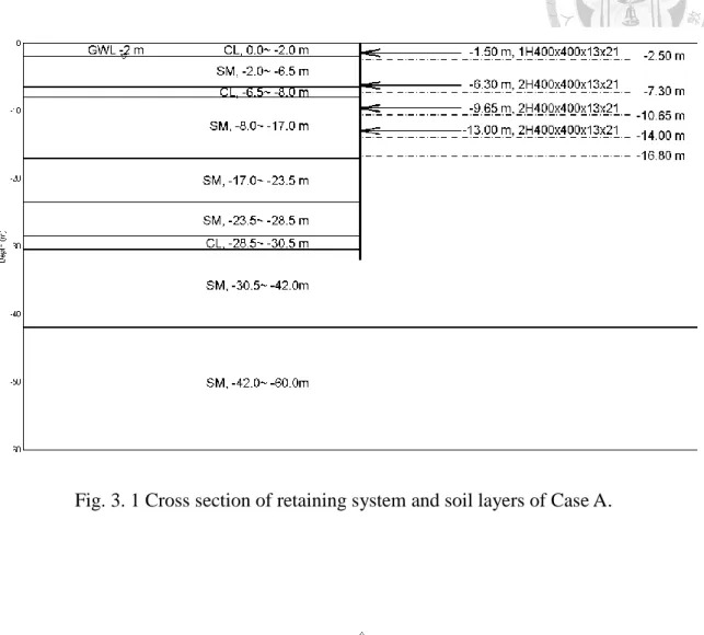
Case A located in Kaohsiung, Taiwan, is a rectangular site with length of 70 m and width of 20 m. The depth of excavation is 16.8 m, implemented by the bottom-up construction method and retained by diaphragm wall with thickness of 0.9 m and 32 m deep. There are 5 stages of excavation and the diaphragm walls were propped by struts at 4 levels. The relative positions of each excavation surfaces, struts, and soil layers are shown in Fig. 3.1, while the soil profile are shown in Table 3.1. There were 4 inclinometers set in the middle of each side of diaphragm wall to monitor the wall deformation, as indicated in Fig. 3.2, and the measurements of inclinometer are shown in Fig. 3.3. Construction site information and in situ measured data in Case A were obtained from Dao (2015).

The raw measured inclinometer data are slopes of diaphragm wall at different depth, and the toes of diaphragm wall were usually adopted as the reference points of the measurements of inclinometers. As can be seen in the Fig.3.3, the deflections of toes are zeros. According to Hwang et al. (2007), the connecting points where the first or

(34)

second level of struts jointed the diaphragm wall are more stable than the toe, and they are more suitable to be the reference points of inclinometer measurements. Therefore, the correction method following by Hwang et al. was applied to Case A, shown in the Fig. 3.4.

As can be seen in Table 3.1, soil types of Case A are primarily sand except three thin clayey layers. It is concluded that sandy layers would dominate the behavior of wall deformation in Case A. The Mohr-Coulomb model was used and the parameters of the soil model are listed in Table 3.2 on the basis of Dao (2015). In the Table 3.2, the effective Young’s modulus of sand was decided by following equation after Hsiung (2009).

) ( 2000

' N kPa

E 

where N is the blow number of standard penetration test (SPT). The undrained Young’s modulus of clay layer can be obtained by the following empirical equation as reported by Bowles (1996), Lim et al. (2010), Likitlersuang et al. (2013), Khoiri and Ou (2013).

u

u S

E 500

Three finite element analyses were carried out, including 1 three dimensional model and 2 two dimensional models for different sections, shown in Fig. 3.5. The sections of two dimensional simulations are shown in Fig. 3.5 b, c and d.

According to the displacement result of simulations shown in Fig. 3.6, apparently,

(35)

is, the length of diaphragm wall in out-of-plane direction was assumed to be infinite long, the width of excavation, which is the distance of the walls in section in Fig. 3.5 b and c., became one of most important factor affecting the amount of wall deflections.

3.2 Case B

Case B is located in Taipei, Taiwan, with an irregular site shape and was constructed by the top-down method. There are 6 stages of excavation propped struts or floor slabs at 5 level (Fig. 3.7 and Fig. 3.8), and the soil profile is shown in Table 3.3.

The longest side of Case B has a length of 50.5 m with a diaphragm wall thickness of 1 m and depth of 36 m. The excavation was 19.6 m deep. Case B is adjacent to Songshan-Xindan line and Zhonghe-Xinlu line of Taipei MRT system; therefore, the wall deflection was regulated by law strictly. According to “Regulation on Building Restrictions along MRT Facilities”, the excavations near the MRT system must not cause any deflection of tunnel over 20 mm and deformation of rails over 10 mm.

Therefore, Case B used much stiffer retaining system, including 16 wall piles to depth of 45 m, 4 buttress walls and 3 cross walls, as shown in Fig. 3.9.

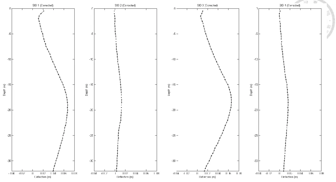
The construction procedures of Case B are complicated. It was divided into two zones, MRT side and warehouse area (Fig. 3.9), with different excavation procedures shown in Fig. 3.7 and Fig. 3.8. There are 7 inclinometers set on each side of excavation (Fig. 3.9), where the measured deflections of the walls were shown in Fig. 3.10.

According to Hsieh et al. (2016), the diaphragm wall around SID 1 was co-constructed with four wall piles to bear the weight of superstructure, and the four inclined steel columns for the top-down construction method were designed. Therefore, it was observed that the diaphragm wall around SID 1 kept deflecting outward after the first stage of excavation.

(36)

In Case B, the Mohr-Coulomb model were used with the parameters listed in Table 3.4. All of the site information and in situ measured data in Case B were provided by Trinity Foundation and Engineering Consultants, Co. Ltd.

In additional to Plaxis 3D analysis, the one-dimensional elastoplastic foundation beams analysis software TORSA (Taiwan Originated Retaining Structure Analysis) was also used.

The results of wall deformations show in Fig. 3.11. The finite element model was simplified for accelerating computation in Case B, i.e. the co-construction of diaphragm wall and wall piles was set vertically, but it can still react to the three dimensional effect.

The measured data shown in Fig. 3.10 and Fig. 3.11 was not corrected due to lack of complete wall deformation data at each construction stage. Therefore, the inclinometer correcting method in Case A cannot be applied here. As mentioned earlier, the diaphragm wall deformed shape can be obtained by inclinometers, but its displacement depends on the reference point we selected. Therefore, the wall deformed curves were shifted to match the toe displacements for the result of TORSA and Plaxis 3D separately, as shown in Fig. 12 and Fig. 13. It can be seen that three dimensional finite element method still works better because the three dimensional effect was involved in

(37)

Fig. 3. 1 Cross section of retaining system and soil layers of Case A.

Fig. 3. 2 Plane view of monitoring equipment in Case A.

(38)

(39)

Fig. 3. 4 Corrected wall deformations obtained by inclinometers in Case A.

(40)

(41)

Fig. 3. 6 Wall deformations obtained by measurements and simulations in Case A.

(42)

(43)

Fig. 3. 8 Cross sections of warehouse district retaining system in Case B.

(44)

(45)

Fig. 3. 10 Wall deformations obtained by inclinometers in Case B.

(46)

(47)

Fig. 3. 12 Wall deformations shifted to match Plaxis result.

(48)

(49)

Table 3. 1 Soil profile of Case A.

Depth (m) Soil Type γt (kN/m³) SPT N φ’ (Deg) c (kPa)

0.0-2.0 CL 19.3 6-7 29 28

2.0-6.5 SM 20.9 5-11 32 -

6.5-8.0 CL 19.7 3-4 30 21

8.0-17.0 SM 20.6 5-17 32 -

17.0-23.5 SM 18.6 5-17 32 -

23.5-28.5 SM 19.6 5-17 33 -

28.5-30.5 CL 18.6 11-15 32 84

30.5-42.0 SM 19.6 18-26 34 -

42.0-60.0 SM 19.6 28-42 34 -

(50)

Table 3. 2 Soil parameters of Case A for Mohr-Coulomb model.

Depth (m) Soil Type γt (kN/m³) φ’ (Deg) c (kPa) E’ (MPa) υ’ ψ’ (Deg) K0 Su (kPa) Eu (MPa) υu

0.0-2.0 CL 19.3 - - - 28 14 0.495

2.0-6.5 SM 20.9 32 0.5 16 0.3 2 0.47 - - -

6.5-8.0 CL 19.7 - - - 21 10.5 0.495

8.0-17.0 SM 20.6 32 0.5 22 0.3 2 0.47 - - -

17.0-23.5 SM 18.6 32 0.5 22 0.3 2 0.47 - - -

23.5-28.5 SM 19.6 33 0.5 22 0.3 3 0.46 - - -

(51)

Table 3. 3 Soil profile of Case B.

Depth (m) Soil Type γt (kN/m³) SPT N φ’ (Deg) c (kPa)

0.0-7.9 CL 18.7 3-7 30 24.5-34.3

7.9-17.1 SM 19.4 11-24 32 -

17.1-20.3 CL 18.9 4-12 30 63.8

20.3-29.3 SM 19.2 10-38 33 -

29.3-39.5 CL/ML 18.6 9-23 32 117.7

39.2-41.4 SM 19.7 22-26 33 -

41.4- GW 21.1 50 38 -

(52)

Table 3. 4 Soil parameters of Case B for Mohr-Coulomb model.

Depth (m) Soil Type γt (kN/m³) φ’ (Deg) c (kPa) E’ (MPa) υ’ ψ’ (Deg) Su (kPa) Eu (MPa) υu

0.0-7.9 CL 18.7 30 0 - - - 24.5-34.3 19.6 0.495

7.9-17.1 SM 19.4 32 - 39.2 0.3 2 - - -

17.1-20.3 CL 18.9 30 0 - - - 63.8 34.3 0.495

20.3-29.3 SM 19.2 33 - 49.1 0.3 3 - - -

29.3-39.5 CL/ML 18.6 32 0 - - - 117.7 54.0 0.495

39.2-41.4 SM 19.7 33 - 61.3 0.3 3 - - -

(53)

Chapter 4 Geometry Study

Eight factors, including excavation depth, wall depth, thickness of wall, length and width of excavation, difference of water head between inside and outside of excavation, average horizontal and vertical spacing of struts play significant roles in system stiffness of a deep excavation when three dimensional effect is considered.

Except for the factors mentioned above, other factors remained constant during analyses. In all of the geometry study, only single-layered sandy stratum was used and the soil parameters were unchanging. The H beam with dimension of 300 mm  300 mm  10 mm  15 mm was used in each level of struts and pre-stressed to 490.5 kN (compression). The details of soil, wall, and struts parameters are listed in the Table 4.1.

According to Roboski (2004), the boundaries were set ±5He (five times the excavated depth) to eliminate the boundary effect. A denser mesh was used inside the excavation and looser on the outside, on the basis of Ou et al. (1996).

The setting value of each factor was explained in the following section.

4.1 The Geometry Parameters

4.1.1 Excavation Depth (H

e

) and Wall Depth (H)

There are two groups, Groups A and B, for different He and H in geometry study.

According to normal depth of excavation for commercial building in Taiwan, excavation depths were set 20 m in Group A. A typical depth excavation for commercial building in Taiwan is around 20 m. The ratio of wall depth to excavation depth in a range usually depends on the soil type of excavation, i.e. 1.7 to 2.0 for sandy soil, 2.2 to 2.5 for clayey soil, and about 1.6 for gravelly layer. Therefore, H was selected to be 40

(54)

For the Group B, He = 30 m and H = 60 m were used. This group is used for figuring out the three dimensional effect more comprehensively, though He and H are seldom reaching that value in practice.

4.1.2 Average Horizontal (H

h

) and Vertical Spacing of Struts (H

v

)

The average vertical spacing of struts (Hv) is related to the number of excavation stages as the level of each strut is normally set 1 m above the previous stage of excavation. Therefore, the number of construction stages depends on Hv. The value of Hv were set as 2.73 m, 3.33 m, 4.29 m for Group A and 2.86 m, 3.33 m, 4 m for Group B.

The average horizontal spacing of struts (Hh) were set to be 4 m, 5 m and 6m for both groups, which are the most common spacing used in Taiwan. Because the length and width of excavation are not always dividable by Hh, the following formula was used to calculate the number of struts needed:

) (L_w H_h floor

N 

where N is the number of struts and Lw is the length or width of the excavation, depends on which side is calculated. The operator “floor” is used to round down (L _w H_h) to an integer.

The horizontal positions of struts were calculated following the equation.



1





L S N

R

(55)

could make S accurate to one decimal point.

As can be seen in the formulae above, the Hh would become Lw/N, but not equal to the Hh set previously. The Hh, after the processes above, is in the range between 2.67 m and 5.92 m for Group A and between 3 m and 5.94 m for Group B.

4.1.3 Maximum Water Head Difference (H

w

)

In practice, the ground water table inside the excavation should be maintained about 1 m below the surface of the following excavation. The ground water table is about 2 m to 6 m below the ground surface in Taipei basin; therefore, the lowering of the ground water table inside the excavation is necessary. However, the dewatering would lead to a higher water head difference between the inside and the outside of the excavation, where the large water pressure would have the diaphragm wall deformed.

The final excavation surfaces are 20 m for Group A and 30 m for Group B, while the final ground water tables inside the excavation are 21 m and 31 m, respectively. The ratio of the maximum water head difference to the excavation depth

e w

H

H were selected

to be 0.95, 0.7 and 0.45. To simplify the model, the level of outer ground water table did not drop accordingly during the construction. Instead, it remained constant throughout the entire time.

4.1.4 Thickness of Wall (D)

The thickness of wall, in a typical design, is about 5 percent of the excavation depth. To examine the influence of the wall stiffness to the three dimensional effect, the wall of 0.5 m, 1.8 m and 1.2 m thick were used in the simulations.

4.1.5 Dimensions of Excavation (L and B)

All of the excavation sites in the geometry study were rectangular ones. L is the

(56)

dimensional model, the primary and complimentary walls could be switched to obtained more simulation results. In other words, the primary wall is not always the longest one.

It depends on which wall deformation is to be observed, and the complimentary wall is the one next to it.

In the work done by Finno et al. (2007), the three dimensional effect become insignificant when the ratio of the excavation length to depth (

He

L ) over 6. They also

indicated that the excavation length to width ratio (_B^L ) has some influence on PSR.

Therefore, _B^L and

He

L were used to determine the dimensions of excavation for the

simulations.

Firstly,

He

L were set to be 0.5, 1.0, 1.5, 2.0, 2.5 and 3.0, respectively. Secondly,

B

Lwere set to be 0.5, 0.7, 1.1, 1.3 and 1.7. Therefore, 30 sets of excavation dimensions were determined. Considering the exchange of the primary and complimentary wall,

He

L and _B^L can vary from 0.29 to 6 and 0.5 to 2, respectively. More details on the dimensions of excavation can be seen in Table 4.2 and Table 4.3.

The factors mentioned above except L and B are shown more briefly in Fig.4.1, and the mesh density of finite element model could be seen in the Fig.4.2.

4.2 Results and Discussions

(57)

correlation coefficient. Then the power terms were accordingly adjusted to optimize a convergence of the proposed equation for the system stiffness. After several trials, the proposed new system stiffness S1 is formulated as follows.



 







 ₂_.₈ ₁_.₇¹^.⁸ ₀_.₈²^.¹ ₀_.₈ ₀_.₉

1 log

h v w

e H L B H H

H

D S H

The effects of L and B were illustrated in Fig.4.3. The width of the excavation B depended on_B^L . In the other words, B increased while L became greater. In order to

minimize the effect of L, the ratio _L^B was used to clarify the effect of B. It can be seen from the vertical and horizontal positions of points that L has great influence on wall deformation and S1 can distinguish various L clearly. In B, the influence is blurred, therefore a lower power term of B was given according to the correlation coefficient.

The horizontal and vertical spacing of struts, Hh and Hv, have relative lower influence on wall deformation. As can be seen in Fig.4.4, the vertical positions of points had not much differences with Hh and Hv changing. Therefore smaller power terms should be given.

The thickness of wall, D, and normalized maximum water head difference,

e w

H

H , had

significant influence on wall deformation, shown in Fig. 4.5. However, the total result would diverge if the power terms were too large, especially

e w

H

H . The moment of inertia

of diaphragm wall,^{I } ^LD₁₂³, was used in numerator of the system stiffness defined by Clough et al. (1989), so we set the initial value of power of D to 3. There is no formula of system stiffness including

e w

H

H , hence the initial value of power of

e w

H

H was set arbitrarily. Finally we started the processes of trial and error with those initial value.

Due to _H^H remain constant, the figures of He and H would be the same, hence

(58)

only He was shown in Fig.4.6. For the same reason as

e w

H

H He and H also needed the processes of trial and error with arbitrary initial value.

As the proposed system stiffness S1 came out, a new design chart was plotted with S1 versus the maximum deformation of wall normalized by excavation depth (Fig.4.7), the fitting result with sum of squared error (SSE) equals 43.32 and R-square equals 0.97 was also shown.

The proposed design chart was divided and re-colored by different factors to examine the performance. In Fig.4.8, the chart was divided into 3 parts with different range of L and colored by _L^B . The darker color of markers represent the higher value

of ^B_L . It was found that the darkest markers (_L^B =2.0) located in the lower part of stripe while L = 31 m to 60 m, but it changed to upper part of stripe as L = 64 m to 180 m.

That is, there are some interactions between L and _L^B . Again, the chart was divided into 3 parts with different

e w

H

H and colored by other

factors, seen in Fig.4.9 to Fig.4.11. It can be seen that the distributions of other factors are quite the same in different

e w

H

H . In the other words,

e w

H

H only affected how long the exponential tendency developed, but it had no interactions with other factors.

In Fig.4.7, the red point on left side represented the wall deformation on the long

(59)

extreme large and small cases, e. g. excavation with dimension of 90 m by 180 m retained by diaphragm wall with D = 0.5 m, Hv = 4 m and Hh = 6 m, and excavation with dimension of 10 m by 6 m retained by diaphragm wall with D = 1.2 m, Hv = 2.73 m and Hh = 2.67 m.

Those extreme cases would cause bias on the result of regression, especially the weight of each case in regression is equal, and therefore another proposed system stiffness S2 came out. The definition of the proposed system stiffness S2 was shown following:



 







 ₃_.₅ ₂_.⁰₆^.⁹ ₀_.₈²^.⁷ ₁_.₁ ₁_.₁

2 log

h v w

e H L B H H

H

D S H

New regression analysis was conducted on those cases whose L is between 20 m and 71 m, shown in Fig.4.12. The fitting result with SSE equals 10.53 and R-square equals 0.98 was also shown.

It can be seen that the new regression equation worked better than the last one. The equation overestimated the wall deformation about 0.4 mm and 18.6 mm on the long side and short side, separately.

It should be noted that the regression results are only suitable for top-down excavations in sandy soil without cross wall and buttress wall due to the models used in this study.

(60)

(61)

Fig.4. 2 The mesh density of finite element model.

(62)

(63)

Fig.4. 4 The performance of S1 on Hv and Hh.

(64)

(65)

Fig.4. 6 The performance of S1 on He.

(66)

(67)

Fig.4. 8 Design charts of different range of L colored by B/L.

(68)

(69)

Fig.4. 10 Design charts of different Hw/He colored by Hv and Hh.

(70)

(71)

Fig.4. 12 New design charts with S2 versus deformation.

(72)

Table 4. 1 Parameters of soil, wall, and struts.

Unit Value

Soil

γ kN/m³ 20

E’ kN/m² 50000

υ’ - 0.3

c’ kN/m² 0

φ’ ° 30

ψ º 0

Wall

γ (*) kN/m³ 4

E’ kN/m² 24630000

υ’ - 0.2

Struts

EA kN 2438000

*NOTE: According to manuals of PLAXIS, the plate element itself does not occupy any volume and overlaps with the soil elements. It might be considered to subtract the unit soil weight from the real unit weight of plate to compensate for the overlap. Hence, the

(73)

Table 4. 2 Dimensions of excavations in Group A.

L/He

0.5 1.0 1.5 2.0 2.5 3.0

L/B L B B/He L B B/He L B B/He L B B/He L B B/He L B B/He

0.5 10 20 1.00 20 40 2.00 30 60 3.00 40 80 4.00 50 100 5.00 60 120 6.00 0.7 10 14 0.71 20 29 1.43 30 43 2.14 40 57 2.86 50 71 3.57 60 86 4.29 1.1 10 9 0.45 20 18 0.91 30 27 1.36 40 36 1.82 50 45 2.27 60 55 2.73 1.3 10 8 0.38 20 15 0.77 30 23 1.15 40 31 1.54 50 38 1.92 60 46 2.31 1.7 10 6 0.29 20 12 0.59 30 18 0.88 40 24 1.18 50 29 1.47 60 35 1.76

(74)

Table 4. 3 Dimensions of excavations in Group B.

L/He

0.5 1.0 1.5 2.0 2.5 3.0

L/B L B B/He L B B/He L B B/He L B B/He L B B/He L B B/He

0.5 15 30 1.00 30 60 2.00 45 90 3.00 60 120 4.00 75 150 5.00 90 180 6.00 0.7 15 21 0.71 30 43 1.43 45 64 2.14 60 86 2.86 75 107 3.57 90 129 4.29 1.1 15 14 0.45 30 27 0.91 45 41 1.36 60 55 1.82 75 68 2.27 90 82 2.73 1.3 15 12 0.38 30 23 0.77 45 35 1.15 60 46 1.54 75 58 1.92 90 69 2.31 1.7 15 9 0.29 30 18 0.59 45 26 0.88 60 35 1.18 75 44 1.47 90 53 1.76

(75)

Chapter 5 Conclusions and Recommendations

From the work carried out in this study, several conclusions and recommendations can be drawn herein.

5.1 Conclusions

1. Wall deformations in large excavations.

As can be seen in Fig.4.3, the stripe got wider while L increased, especially for L ranging from 64 m to 180 m. It was found that _L^B attributed the width of stripe in large L most, seen in Fig.4.8.

As mentioned in chapter 4, the influence of _L^B is not clear. The distribution

of different _L^B would change with the increment of L.

2. The influence of maximum water head differences on wall deformation.

The maximum water head difference is the only factor which is not one of the geometry configurations. However, as can be seen in Fig.4.3 to Fig.4.6, it has greatest influence on wall deformation.

However,

e w

H

H only affected how long the exponential tendency developed, but it had no interactions with other factors.

3. Performance of new system stiffness.

The new system stiffness, S1 and S2, worked much better on the long side than short side. We thought that it is because the influence of B is not clear in those form of system stiffness, as mentioned previously. On the long side of excavation, which had lower B, the wall deformation were affected by B less than short side.

That is one of the deficiencies of new system stiffness.

(76)

5.2 Recommendations

In this study, four factors, including

e w

H

H , soil profile, struts types and prestress,

were not considered.

e w

H

H was fixed as 2.0 in this study. For the future work, it can be examined with various diaphragm wall thickness D. The soil profile is also important. The soil profile in this study was limited to sandy soil. To make a design chart more extensively used, clayey soil should be taken into considerations, and multi-layered stratum could be simplified as average sandy and clayey soil parameters.

In practice, the strut pre-stress is usually applied about 50% of the allowable axial strength of struts, except on the first level of supports. The variations of struts types and pre-stress could be involved to make estimation of design chart more precise, but it might cause the chart too complicated to use.

The factors should be normalized before figuring out the power terms of them to obtain a dimensionless system stiffness for more general application.

Advanced soil constitutive models, capable of mimicking the nonlinear stress-strain behavior, shear dilatancy, loading-unloading hysteresis etc., can be used to simulate the behavior of excavation more precisely. Lastly, the influence of B on diaphragm wall deformation should be further examined.

(77)

REFERENCE

[1] Bowles, J. E., (1996). “Foundation Analysis and Design”. 5^th Edition, McGraw-Hill Book Company, New York, USA.

[2] Bryson, L. S., and Zapata-Medina, D. G. (2012). “Method of Estimation System Stiffness for Excavation Support Walls”. Journal of Geotechnical and Geoenvironmental Engineering, Vol. 138, 1104-1115.

[3] Chua, H. Y., and Bolton, M. D. (2005). “Modeling of Horizontal Arching on Retaining Walls”. International Conference on Soil Mechanics and Geotechnical Engineering, Vol. 3, 1455-1459.

[4] Dao, S. D. (2015). “Application of Numerical Analysis for Deep Excavations in Soft Ground”. Taiwan, National Kaohsiung University of Applied Sciences.

[5] Finno, R. J., Blackburn, J. T., and Roboski, J. F. (2007). “Three-Dimensional Effects for Supported Excavations in Clay”. Journal of Geotechnical and Geoenvironmental Engineering, Vol. 133, 30-36.

[6] Finno, R. J., Bryson, L. S., and Calvello, M. (2002). “Performance of a Stiff Support System in Soft Clay”. Journal of Geotechnical and Geoenvironmental Engineering, Vol. 128, 660-671.

[7] Finno, R. J., Calvello, M. (2005). “Supported Excavations: Observational Method and Inverse Modeling”. Journal of Geotechnical and Geoenvironmental

Engineering, Vol. 131, 826-836.

[8] Hsieh, H. S., Cherng, J. C., and Huang, H. F. (2010). “A Note on the Diaphragm Wall Design for Small/Medium Size Excavations”. Sino-Geotechnics, No.123, 15-22.

(78)

[9] Hsiung, B. B. C. (2009), “A Case Study on the Behavior of a Deep Excavation in Sand”. Computers and Geotechnics, Vol. 36, 665-675.

[10] Khoiri, M., and Ou, C. Y. (2013). “Evaluation of Deformation Parameter for Deep Excavation in Sand through Case Studies”. Computers and Geotechnics, Vol. 47, 57-67.

[11] Lee, F. H., Yong, K. Y., Quan C. N., and Chee, K. T. (1998). “Effect of Corners in Strutted Excavations: Field Monitoring and Case Histories”. Journal of

Geotechnical and Geoenvironmental Engineering, Vol. 124, 339-349.

[12] Likitlersuang, S., Surarak, C., Wanatowski, D., Oh, E., and Balasubramaniam, A.

(2013). “Finite Element Analysis of a Deep Excavation: A Case Study from the Bangkok MRT”, Soil and Foundations, Vol. 53, No. 5, 756-773.

[13] Lim, A., Ou, C. Y., and Hsieh, P. G. (2010). “Evaluation of Clay Constitutive Models for Analysis of Deep Excavation under Undrained Conditions”. Journal of GeoEngineering, TGS, Vol. 5, No. 1, 9-20.

[14] Marr, W., and Hawkes, M. (2010). “Displacement-Based Design for Deep Excavations”. Earth Retention Conference, Vol.3, pp. 82-100.

[15] Meng, L. J., Zhang, Y. J., and Ma, X. W. (2015). “A Numerical Analysis Method for Active Earth Pressure behind a Retaining Wall Considering Soil Arching Effect”. Electronic Journal of Geotechnical Engineering, Vol. 20, Bund. 8.

(79)

Excavations-Establishment of a Forecast Model for Taipei Basin T2 Zone”.

Journal of Marin Science and Technology, Vol. 18, No. 1, 1-11.