動態物流輸配送---資源分配管理模式

行政院國家科學委員會專題研究計畫 成果報告

動態物流輸配送-資源分配管理模式

中 華 民 國 94 年 9 月 28 日

A Novel Dynamic Resource Allocation Model for Demand-Responsive City Logistics Distribution Operations

(accepted by Transportation Research Part E; SCI, SSCI)

Jiuh-Biing Sheu

Institute of Traffic and Transportation National Chiao Tung University 4F, 114 Chung Hsiao W. Rd., Sec. 1

Taipei, Taiwan 10012 R.O.C.

TEL: 886-2-2349-4963 FAX: 886-2-2349-4953 jbsheu@mail.nctu.edu.tw

Abstract

This paper presents a dynamic customer group-based logistics resource allocation methodology for the use of demand-responsive city logistics distribution operations. The proposed methodology is developed based on the following five developmental procedures, including: (1) specification of demand attributes, (2) customer grouping, (3) customer group ranking, (4) container assignment, and (5) vehicle assignment. The numerical results show that the model permits managing both the time-varying customer order data and logistics resources dynamically with the goal of optimal logistics resource allocation. Particularly, both the aggregate operational costs and average lead time are reduced by 27.4% and 8.7%, respectively, in a case study.

Key Words: Fuzzy clustering, Fuzzy ranking, Optimal assignment, Dynamic programming,

1. Introduction

Dynamic logistics resource allocation, referring to the mechanism of allocating logistics resources, e.g., containers and vehicles, in quick response to the variety of customer order demands changing in short-term time intervals, is of vital importance to efficient demand-responsive city logistics distribution operations. In fact, recent advances in information and communication technologies have significantly altered the consuming behavior of end-customers, and aroused their desire for quick response from the vendor enterprises. Facing such induced issues as distribution channel restructuring and quick response to the diversity of customer order demands, the specialized city logistics companies have been urgently requested with the capability of allocating limited resources, efficiently and effectively, in the process of city logistics distribution operations. One striking example is found in our study case, where a specialized city logistics enterprise has encountered a serious resource allocation problem resulting from the request of a contracted tele-shopping company to not only manage the corresponding inventories but also provide quick-responsive door-to-door logistics services to the corresponding end-customers. Accordingly, dynamic allocation of logistics resources defines the feasibility of an efficient demand-responsive city logistics distribution system by enhancing the resource utility as well as by shortening the pre-route work process time in quick response to changes in customer demands.

Despite the importance of dynamic logistics resource allocation in demand-responsive city logistics distribution operations, studies in terms of incorporating such a mechanism into the comprehensive scheme of demand-responsive city logistics distribution operations are rather limited in previous literature. In contrast, most previous research appears to focus mainly on the en-route freight transportation problems, e.g., vehicle routing problems (VRP), and the corresponding fleet management problems (Altinkemer et al., 1990; Bramel et al., 1995; Gendreau et al., 1996; Powell, 1987; Powell et al., 1997, 2002; Mahmassani et al., 2000;

Secomandi, 2000). Among these, two typical VRP-induced problems, including the inventory routing problems (IRP) and multi-commodity fleet management problems are illustrated below for discussion.

Essentially, IRP, which is also termed as the vendor-managed distribution system in recent literature (Beltrami et al., 1974; Burns et al., 1985; Federgruen et al., 1986; Blumenfeld et al., 1987; Dror et al., 1987; Larson, 1988; Webb et al., 1995; Herer et al., 1997; Larsen, 2001; Ghiani et al., 2003), can be regarded as an enrichment of vehicle routing problems (VRP) to consider customers’ inventory factors, such as storage capacity, consumption characteristics and the consequences of stockouts in determining logistics distribution strategies. Such an idea of incorporating both supply-oriented routing and demand-oriented inventory considerations in a logistics distribution system was first proposed by Beltrami et al. (1974), followed by some literature which aimed to minimize either the fleet size required for goods delivery in the strategic domain (Larson, 1988; Webb et al., 1995) or the corresponding distribution costs in the operational domain (Burns et al., 1985; Federgruen et al., 1986; Blumenfeld et al., 1987; Dror et al., 1987; Herer et al., 1997). As noted in Dror et al. (1987), one distinctive feature of IRP models is the ability to ensure that none of the customers run out of the commodity at any time in the planning horizon of logistics distribution, and accordingly, it seems that IRP may be more practical for the operations of demand-responsive logistics distribution, relative to classical VRP approaches.

Although the aforementioned demand-driven operational factors are considered in the existing IRP models, the issues of multiple logistics resource allocation in the supply domain still remain in the corresponding model formulation process. It is noteworthy that most classical IRP models aim to define the corresponding inventory costs, e.g., holding costs and shortage costs, incurred in the demand side rather than the supply side. And thus, it may contribute to the inadequacy of the existing IRP models in characterizing the dynamics of

logistics resources as well as their capability in allocating the corresponding resources for quick response to short-term changes in customer demand patterns.

In contrast to prior IRP approaches, which attempt to incorporate customers’ replenishment requirements into routing problems, studies of multi-commodity fleet management concentrate particularly on the supply side regarding the utilization of vehicular fleets and the corresponding resource assignment so as to match the given customer demands characterized with either deterministic or stochastic features (Shan, 1985; Chih, 1986; Powell, 1986, 1987; Crainic et al., 1993; Gendron et al., 1995; Cheung et al., 1996; Powell et al., 1997, 2002; Hall, 1999; Chan et al., 2001; Godfrey et al., 2002a, b; Leung et al., 2002; List et al., 2003). For instance, the issue of empty container reallocation under demand uncertainty was tackled in Crainic et al. (1993), and followed by Gendron et al. (1995), which considered both the loaded container delivery and empty container reutilization issues for heterogeneous container fleet management of maritime shipping companies. The distinctive feature of these two models is the ability to integrate the allocation of empty containers into classical loaded container delivery problems, and then solve it with relatively efficient algorithms for managing system-wide heterogeneous resource allocation. Similar concepts are applied in Hall et al. (1999) to deal with empty truck problems in a less-than-truckload (LTL) trucking network, where the effects of empty truck movements are referred to as imbalance costs in fleet management. A more general model of resource allocation can also be found in McGinnis (1997), which regards sizing vehicle fleets as a specific example of sizing system-wide reusable resources.

In addition, there is a growing attempt in recent literature to investigate the issues of assigning pre-determined multiple commodities to multiple types of vehicles and corresponding resources (Powell et al., 1997, 2002; Mahmassani et al., 2000; Godfrey et al., 2002a, b; Smilowitz et al., 2003). Among those studies, fleet management is tackled

specifically with network-wide commodity-based flow problems, involving both intra-node and inter-node physical distribution activities, such as vehicle loading and routing, respectively. Furthermore, the deferred item and routing problem (DIVRP) addressed in Smilowitz et al. (2003) can be regarded as a special case of the aforementioned multi-commodity flow problems since it deals specifically with delivering deferred items by different types of transportation modes to improve the utility of transportation modes in a distribution network. Nevertheless, in-depth investigation in the nature of delivery-commodity attributes and their dynamic effects on allocating logistics resources before the phase of vehicle dispatching appear limited in the previous literature. Furthermore, the computational efficiency under large-scale network flow conditions also remains to be a difficult challenge.

Based on the literature review, several generalizations are summarized in the following to clarify the significance of this study.

(1) In the field of traditional freight transportation, there is an extensive amount of literature in relation to VRP and container/truck assignment for multi-commodity multi-modal transshipment problems. However, techniques of clustering customer orders dynamically and integration with multi-resource assignment for logistics distribution operations are scarce. In most early literature, the customer demands were assumed to be known with either deterministic or stochastic properties, and then input directly into a global optimization model for multi-resource assignment. (2) Some early literature of logistics management may shed light on proposing either the

principles of customer grouping or the utilization of classical clustering techniques for route segmentation and fleet management (Fisher et al., 1981; Altinkemer et al., 1990; Bramel et al., 1995, 1999; Ballou, 2002). Nevertheless, their treatments may not be applicable for dynamical logistics resource allocation in response to a variety

of customer order demands in the operational level, as addressed in this study.

(3) Development of multi-objective programming models to deal with the general resource allocation problems can be readily found in the literature (Mine et al., 1979; Chankong et al., 1983; Hussein et al., 1995; Lai et al., 1999; Ross, 2000). However, as maintained previously, the integration with the specific phase of data clustering is rare in the resource allocation literature.

Accordingly, in this study, we propose a comprehensive operational framework together with specific operational models for dynamic logistics resource allocation. Compared to previous literature, the proposed methodology exhibits two distinctive features. First, considering the dynamics of customer demand attributes and their effects on city logistics distribution operations, five sequential phases, including (1) order entry processing, (2) customer grouping, (3) customer group ranking, (4) container assignment, and (5) vehicle assignment, are incorporated into the proposed framework to dynamically allocate multi-type logistics resources prior to vehicle dispatching1. Second, using the phases of customer grouping and ranking, customer order data are dynamically updated and clustered to facilitate inventory assignment and the corresponding resource allocation. Here, employing advanced clustering techniques, e.g., fuzzy clustering approaches, customer orders are efficiently classified into several groups associated with specific service priority to optimize the availability of logistics resources.

The remainder of this paper is organized as follows. The primary procedures for methodology development and the fundamentals of the proposed method are presented in

1 _{In the previous literature, it is found that some multi-resource allocation problems are formulated with globally}

optimized models. Nevertheless, some assumptions in terms of the problem definition either in the demand side or supply side are needed, and thus may lead these global optimization models too simplified to be true. In addition, the corresponding model formulation with global optimization programming approaches may have some difficulties in searching optimal solutions under conditions of large-scale distribution networks and tremendous customer demand data. Furthermore, these globally optimized models may not have the features of updating and grouping customer orders dynamically in quick response to the diversity of customer orders changing in short-term time intervals. That’s why we formulate such a dynamic logistics resource allocation model with an architecture embedding sequential mechanisms rather than a global optimization model.

Section 2. A numerical study and the corresponding results generated via the proposed method are summarized in Section 3 to demonstrate the feasibility of the proposed method. Section 4 summarizes the concluding remarks.

2. Methodology development

The architecture of the proposed dynamic logistics resource allocation system is composed mainly of five sequential operational phases: (1) order processing, (2) customer grouping, (3) customer group ranking, (4) container assignment, and (5) vehicle assignment. Here phases (1), (2), and (3) refer to the dynamic demand-oriented data processing conducted for the purpose of grouping customer orders with respective service priority. The resulting output is then input to the remaining phases for dynamic optimization in allocating the time-varying logistics resources available. The aforementioned five sequential mechanisms are carried out each time when the database of customer entries is input to trigger a new logistics distribution mission. The corresponding models and algorithms embedded in these operational phases are detailed in the following subsections.

2.1 Order processing

The phase of order processing aims to determine the target customer orders which are processed and served in a given time horizon T. To facilitate model formulation, it is assumed that the cycle time of customer order processing of the proposed logistics system is fixed, and is equal to T. In addition, each given time horizon T is assumed to embed several time steps referring to the headways of vehicle dispatching to serve group-based logistics distribution in the given time horizon T. Correspondingly, the proposed logistics system examines the order entry database at the beginning of each given time horizon T for grouping the customers, and then for multi-step resource allocation and management in that horizon.

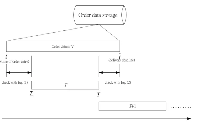
Note that the length of T may depend on the operational conditions of the individual company. To accomplish the aforementioned operational purpose, the current order entry database is examined at the beginning of a given time horizon T (T) with the following collection conditions. L t T L≤ − _i ≤ (1) i t T ≤ (2) where L and L represent the allowable maximum and minimum lead times that the proposed logistics system commits to customers; t and _i t represent the time of order entry _i

and the corresponding delivery deadline associated with a given customer i, respectively; T and T represent the onset and end of the given time horizon T. Equation (1) denotes the

upper bound of the lead time associated with a given customer i, and Eq. (2) is involved to

ensure that the corresponding delivery deadline constraint is not violated. The resulting decision rule of order selection is illustrated in Fig. 1. Using the above collection conditions, the order entry database is examined at T, and those order entries, which satisfy the above collection conditions, are considered for further grouping in the next operational phase. Meanwhile, the remaining order entry database is updated with new order entries for the order processing in the next time horizon.

Fig. 1. Illustration of decision rules for time-varying order selection

2.2 Customer grouping

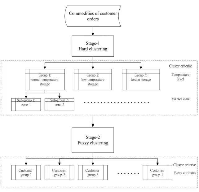
The purpose of this phase is to cluster commodities based on the data of customer order entries identified in the previous phase. Considering the complexity of multi-attribute customer orders, a two-stage customer grouping algorithm is proposed to expedite the corresponding clustering mechanism. The proposed two-stage customer-grouping algorithm

scheme is presented in Fig. 2. The major difference between these two stages is rooted in the nature of criteria used for customer grouping. The first stage clusters the commodities of customer orders using hard criteria, e.g., the temperature level required for reservation and the service zone, and is followed by the second stage, which clusters these commodities in sequence employing fuzzy clustering techniques based on linguistic measures of the

evaluation criteria. Details of the corresponding procedures and models are presented below.

Fig. 2. The proposed two-stage customer-grouping algorithm scheme

In the first cluster stage, two hard criteria, i.e., the required reservation temperature level and service zone, are utilized. The utilization of these two hard criteria is motivated mainly by two factors: container requirements and delivery efficiency, which are considered in practical logistics operations. In general, considering the operational temperature requirement, commodities can be classified into three categories: normal, low-temperature, and frozen goods, where the second and third ones need specific temperature requirements for the reservation in the process of logistics distribution operations. In addition, typical logistics service companies may adopt zone-based delivery service strategies to facilitate vehicle routing and scheduling (Ballou, 2002). Correspondingly, customers are clustered into several groups bounded by specific service zones, based mainly on their locations so as to assign common logistics resources, including containers, vehicles, and drivers, to serve customers in the same groups. Accordingly, both the aforementioned hard criteria are proposed for customer clustering in the first stage.

After the hard clustering in the previous stage, the commodities of customer orders in each hard-clustered group are further clustered using fuzzy clustering techniques, which have extensively been used in diverse areas for either data compression or data categorization (Bezdek, 1973; Cannon et al., 1986; Dave et al., 1992; Frigui et al., 1996; Sheu, 2002; Tao,

2002). Conveniently, the analytical results from our previous research (Hu et al., 2003) have been employed to determine four customer attributes for the use of fuzzy clustering in this stage. They are defined as follows.

(1)_x1 (_k) h

i represents the time difference between the deadline to customer h

i in a given

hard-clustered group h and the current vehicle-dispatching time step k. In real-world

operations, it is permissible to deliver products to those customers associated with close distribution deadlines, and thus, these customers can be categorized into a group that is served by the same vehicular fleet.

(2)_x2(_k) h

i corresponds to the value of the product distributed to customer h

i in a given

hard-clustered group h at a given vehicle dispatching time step k, and to a certain extent it

may depend on the market price of the product. In real-world distribution operations, high-value products may be segmented from other products, and handled with specific security measures for safe delivery.

(3)_x3(_k) h

i represents the external compatibility in terms of the products ordered by customer h

i in a given hard-clustered group h, relative to the products that are scheduled to be

distributed to customers in a given customer group at time step k. This variable is

specified to efficiently provide bulk delivery service to customers in the same group. The higher the external compatibility of products in a given group, the more efficient will be the bulk delivery service in distribution operations.

(4)_x4(_k) h

i represents the internal compatibility in terms of the products associated with a given customer _{i in a given hard-clustered group h at a given vehicle-dispatching time step k.} h In contrast with _x3 (_k)

h

i , ( )

4 _k

x_ih can be used to determine if multiple delivery services are

needed for any given customer.

specific multi-attribute datum used for further fuzzy clustering analysis.

The proposed fuzzy clustering stage is executed through three major procedures, including: (1) binary transformation, (2) generation of fuzzy correlation matrix, and (3) customer grouping. The primary steps executed in the aforementioned procedures are detailed in the following.

Binary transformation

The mechanism of binary transformation aims to transform the customer order attributes collected from the processed order entry data into binary data. Three sequential steps are involved in this mechanism. First, we specified five linguistic terms, including “very high”, “high”, “medium”, “low”, and “very low”, which represent five levels of qualitative criteria to characterize customers’ order attributes. Second, using the order entry data clustered in the previous stage, the attributes associated with each customer order datum were measured using the aforementioned five linguistic terms. Third, based on the mapping relationships presented in Table 1, the linguistic terms associated with the attributes of customers’ orders were transformed into binary codes. As can be seen in Table 1, each linguistic item is represented by a specific set of four bits such as “0000” for the linguistic item “very low”, and “1111” for “very high.” Thereby, each given order attribute p measured from customer

h

i (xp(k))

ih can then be transformed into binary codes with four bits( _, (k))

p j ih σ , which can be expressed as: )] ( ), ( ), ( ), ( [ ) (k _,1 k _,2 k _,3 k _,4 k x p i p i p i p i p ih = σ h σ h σ h σ h (3)

Table 1 Binary transformation of the specified five linguistic terms

To facilitate processing the heterogeneity of customers’ order attributes, the procedure of standardization with respect to ( p_, (k))

j ih

)) ( ( p_, k j ih σ (i.e., ~p_, (k) j ih σ ) is given by ) ( ) ( ) ( ) ( ~ , , _{S k} k k k _p j p j p j i p j i h h σ σ σ = − (4) where p(k) j σ and Sp(k)

j correspond to the values of the mean and standard deviation with respect to p_, (k)

j ih

σ , respectively, and they are denoted by

_h M i p j i p j M k k h h h

∑

(

)

∑

where _{M represents the number of customers in a given hard-clustered group, served at the} h current time step. Therefore, we have the standardized form (~ kxp( )

ih ) associated with each

customer’s order attribute, given by

)] ( ~ ), ( ~ ), ( ~ ), ( ~ [ ) ( ~ 4 , 3 , 2 , 1 , k k k k k x p i p i p i p i p ih = σ h σ σ h σ h (7)

Generation of fuzzy correlation matrix

At this stage, for each hard-clustered group h, a time-varying _Mh_×Mh _{fuzzy correlation} matrix (_Wh(k)_{) is constructed in which each element ( ( )}

, k

w_rh_sh ) represents the correlation

between a given pair of customers _{r and} h _{s . Herein,} h _Wh_{(k) and ( )}

, k

respectively, by

[

]

∑∑

where λ₁ is a parameter which needs to be calibrated to ensure that w_rh_,sh(k) is bounded

with the corresponding upper and lower bounds, i.e., 1 and 0, respectively.

Customer grouping

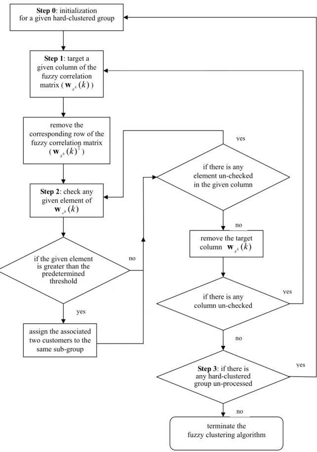
This procedure executes the mechanism of clustering the customers in each given hard-clustered group into several sub-groups with the objective that the customers assigned to the same sub-group are characterized by relatively higher similarity in terms of their attributes, compared to the members in any other sub-groups. Figure 3 presents the proposed customer grouping logic, and the major computational steps are summarized as follows.

Step 0: Initialize the computational iteration for a given hard-clustered group; input the

estimated fuzzy correlation matrix (i.e., Eq. (8)); select a given hard-clustered group h to start the iteration from the first column of the fuzzy correlation matrix (_Wh(k)_{), i.e., letting}

1 = h

s .

h s (i.e., T ) (k h s

w ). Note that the column of the fuzzy correlation matrix associated with the given customer _{s (}h _(k)

h

s

w ) is targeted for the use of clustering other possible customers into the same sub-group. In contrast, the elements of w_sh(k)T are redundant in the

following clustering process, and thus they are removed in this step.

Step 2: Find the largest element in w_sh(k), denoted by w&_rh_sh(k), and then conduct the

following cluster procedures in sequence:

z If the condition w&_rh_sh(k)>λ₂ holds

2_{, then assign customer r to the same sub-group} h

as customer _{s , and remove the row of} h _Wh_{(k) associated with customer r .} h

z Go back to Step 2 to continue checking the other elements of w_sh(k) until there is no

element that meets the aforementioned clustering condition.

z Remove )w_sh(k from (k)

h

W .

z If there are any customers who have not been assigned at this stage, let any given

un-assigned customer be the target customer, and then go back to Step 1 to continue the fuzzy clustering process until all the customers are assigned.

Step 3: Conduct the following termination rules to stop the mechanism of customer grouping:

z If all the hard-clustered groups are processed, then stop the fuzzy clustering algorithm; z Otherwise, select a given un-processed hard-clustered group, and then go back to Step 0

to initialize the fuzzy clustering process for the target hard-clustered group.

2 _{Here, λ}

2 represents a threshold for identifying the relative similarity between a given pair of customers, and is

tentatively set to be 0.7 using trial-and-error tests in this study. In practice, λ2 determines the number of

iteration steps and the number of clusters, both of which exhibit a trade-off relationship in the clustering procedure. For instance, a lower value of λ2 may speed up the clustering procedure as indicated by the reduced

iteration steps; and meanwhile, it may cause a reduced number of customer groups, which loosens the requirement for identifying the mutual similarity of intra-group customers. Accordingly, to avoid any unrealistic clustering results, e.g., an unusually large number of clustered customer groups in queue waiting for delivery services due to inadequate resources, and vice versa, the specification of λ2 should also take into

Fig. 3. Proposed fuzzy clustering logic for customer grouping

2.3 Customer group ranking

After clustering the customer order entries, the next step is to rank the clustered customer groups for their priority of logistics resource allocation. To simplify the computational procedure, the customers’ order attributes in terms of the time difference between vehicle dispatching and delivery deadline and commodity prices (i.e., _x1 (_k)

h

i and ( )

2 _k

x_ih ), together

with the hard-clustering criterion in terms of the reservation temperature level specified in the previous customer grouping stage remain to be the determinants at this stage.

The group ranking estimation procedure contains two main steps. First, each level of reservation temperature ( t ) is associated with a specific weight (ω_t) which is predetermined by logistics operators. In general, the corresponding weight associated with the frozen-temperature level is suggested to be the highest value, followed by the weight associated with the low-temperature level, and then the weight associated with the normal-temperature level, considering the life cycle of goods and specific logistics distribution requirements. Second, the clustered customer groups (g) are ranked by comparing the corresponding group-ranking indexes (δ_g(k)) given by

g g i p p i t g M k x k k g g g

∑ ∑

where ω_tg represents the corresponding weight associated with a given customer group

which needs a specific reservation temperature requirement _{t ;} g g

M represents the number

of customers assigned in a given customer group g; ~ kxp( )

ig represents the quantity of the

integers ranging from 0 to 4 are specified to conveniently quantify the pre-specified five linguistic terms from “very low” to “very high”, respectively. Here the customer order data which are employed to group customer orders are used again to rank the customer groups.

2.4 Container assignment

After ranking the customer groups, this phase triggers the mechanism of assigning appropriate containers to package customer orders with the goals of maximizing the aggregate container loading rate and minimizing the aggregate packaging costs, as presented in Eqs. (11) and (12), respectively. Note that the containers assigned at this stage refer to small-sized containers, e.g., boxes and cases, suitable for city logistics distribution operations. The large-sized containers used for line-haul transportation may be associated with the given freight vehicles, and their corresponding assignment problems are quite similar to vehicle assignment problems, thus are not considered in this phase.

∑ ∑∑

∑ ∑∑

where )CR_jg(k and PC_jg(k) represent the disaggregate container loading rate and the

corresponding packaging costs associated with a given container _{j , which is suitable for the} g use in a given customer group g. Herein, CR_jg(k) and PC_jg(k) are given, respectively,

by

∑

∑

where c represents the corresponding packaging costs when a given container _jg

g

j is

utilized to serve a given customer group g; v_ig_jg is the volume of commodity ordered by a

given customer _{i and served by a given container} g _{j ;} g

g

j

V~ represents the capacity of a given container _{j ; )}g _{Y (k}

g g_j

i is specified as a 0-1 integer decision variable, which is equal to 1 if the commodity of customer _{i is served by container} g _{j at a given time step k;} g otherwise it is 0.

Considering the diverse potential effects of the above two goals (i.e., maximizing the aggregate container loading rate and minimizing the aggregate packaging costs) on the corresponding container assignment problem, two positive weights (i.e., ϖ_CR and ϖ_PC) are introduced. In addition, the difference in measurement scales associated with fill rates and costs may also influence the determination of optimal solutions. Accordingly, the aforementioned container assignment problem is re-formulated as a composite multi-objective optimization problem (U) given by

PC CR

U _{CR PC}

Max =ϖ −ϖ (15)

where ϖ_CR and ϖ_PC are positive, and the sum of these two weights is 1; CR and PC

represent the normalized forms of the corresponding aggregate container loading rate and packaging costs, respectively, and are given by

min max min CR CR CR − − = CR CR (16)

min max min PC PC PC − − = PC PC (17)

In Eqs. (16) and (17), CR_max and PC_max represent the estimates of aggregate container loading rate and the corresponding packaging costs measured in the case in which only the loading-rate maximization problem is considered (i.e., ϖ_CR is set to be 1); and in contrast,

min

CR and PC_min represent the corresponding estimates measured in the case involving the objective function of cost-minimization (i.e., ϖ_PC is set to be 1).

In addition, considering the logistics requirements limited by the corresponding operating capacities, seven respective sets of constraints, shown as follows, are involved in the proposed model.

g j T k g i i j i j j V k Y v g g g g g g × ≤ ∀

∑ ∑∑

∑ ∑∑

∑ ∑∑

∑

∑ ∑∑

∑ ∑∑∑

where θ_ig represents the commodity density associated with the goods ordered by a given

customer _ig_;

g

j

g

i

v represents the total amount of goods ordered by a given customer _ig_; T jg

Q~ represents the total number of a given container _jg _{available in a given time horizon T; and in contrast,}

T g

Q represents the total number of containers available for the use of a given customer group

g in a given time horizon T. Herein, Eqs. (18) and (19) refer to the disaggregate container loading limits in terms of volume and weight, respectively; Eq. (20) is specified to ensure that any given container is assigned to merely serve a single customer, and correspondingly, the case of mixed-order packaging is not permitted in this phase; Eq. (21) implies that the case of multiple containers assigned to a given customer is allowed considering the customers’ large-order cases; Eqs. (22) and (23) represent the corresponding limitations of disaggregate and aggregate container availability in a given time horizon T, respectively; and Eq. (24) denotes the characteristics of decision variables Y_ig_jg(k).

2.5 Vehicle assignment

This phase aims to assign containers resulting from the previous phase to appropriate vehicles under the three goals, i.e., maximizing the aggregate vehicle loading rate (VR), and minimizing both the corresponding aggregate operational costs (OC) and delivery time ( DT ). In addition, one distinctive feature of the proposed model is that in addition to vehicles standing by in the depot, the time-varying proportion of en-route vehicles returning to the depot during a given time horizon T is also considered for the use of vehicle assignment in this phase. Conveniently, the multi-objective optimization based approach is used in this phase, and the corresponding composite objective function (Φ ) is given by

DT OC

VR

Φ _{VR OC DT}

Max =ϖ −ϖ −ϖ (25)

to 1; VR, OC and DT represent the normalized forms of the corresponding aggregate operations vehicle loading rate, operational costs and delivery time, respectively, and are given by min max min VR VR VR − − = VR VR (26) min max min OC OC OC − − = OC OC (27) min max min DT DT DT − − = DT DT (28)

In Eqs. (26) to (28), VR_max represents the estimate of the aggregate vehicle loading rate measured in the case in which the loading rate-maximization problem is considered (i.e., ϖ_VR is set to be 1); and similar treatments are applied to estimate OC_min and DT_min, respectively. In contrast, the other parameters, including VR_min, OC_max, and DT_max, are measured under the corresponding worst cases. Here, VR, OC and DT presented in Eqs. (26) to (28) can be further expressed as

∑ ∑∑

∑

∑ ∑∑

(

)

(

)

∑ ∑∑

∑

where d represents the unit operational costs associated with a given vehicle _lg l, which is

scheduled to serve a given customer group g; g′ represents any given customer group,

which has a relatively higher group-ranking index δ_g′ than δ_g ; G represents the _k

customer sets scheduled to be served at a given time step k; M_g′ and M represent the g number of customer groups g′ and g, respectively; st_g′ and st represent the expected g delivery times associated with customer groups g′ and g, respectively; Z_gl(k) is specified as a 0-1 integer decision variable, which is equal to 1 if a given customer group g is served by vehicle l at a given time step k; otherwise it is 0.

In addition, considering the limitations in terms of vehicle availability and the corresponding capacity associated with each type of vehicle, several sets of constraints, shown as follows, are involved in the proposed model.

k U k Z V N k l l gl k N l g j j l l g g× ≤ ∀      

∑

∑ ∑ ∑

∑∑

∑∑

where U~_l represents the capacity of a given vehicle l; θ_jg represents the density of a given

container _{j ;} g l

Θ~ represents the loading weight limit associated with a given vehicle l; )

(k

the proposed model, N_l(k) is dynamic, and determined at each given time step k by the number of available vehicles remaining at the previous time step k-1 (N_l(k−1)) coupled with the expected number of en-route vehicles which may return to the depot before the end of the current time step k. Accordingly, we have N_l(k) given by

(

)

[

]

(

)

{

}

where N~ represents the total number of available vehicles; σ(k) is the time-varying possibility with which any given en-route vehicle may return to the depot at a given time step

k; and ε represents the maximum allowable error percentage associated with the estimation

of σ(k) . Note that under the intelligent transportation systems (ITS) operational environment, the positions of en-route vehicles can be readily monitored through related information technology, e.g., global positioning systems (GPS) and two-way communication systems, thus leading to the availability of the aforementioned en-route vehicle information. In the aforementioned constraints, Eqs. (32) and (33) represent the aggregate and disaggregate loading capacity limits of vehicles, respectively; in contrast, Eq. (34) denotes the disaggregate loading weight limit associated with each given vehicle, and Eq. (35) specifies the mathematical characteristics of decision variables Z_gl(k) mentioned previously.

Note that once the aforementioned logistics resources allocation mechanisms are executed, the corresponding output results can be readily integrated with any existing vehicle routing model to solve the corresponding vehicle routing problem for each customer group without any extra burden and incompatible problem. This is the reason for proposing the incorporation of such a sophisticated logistics resource allocation method into a comprehensive logistics distribution framework in spite of remarkable advances that have been made in previous literature to improve vehicle routing problems.

3 Numerical results

The main purpose of this numerical study is to demonstrate the potential advantages of the proposed dynamic logistics resource allocation methodology used in a practical logistics distribution case, relative to the existing strategies. The case study examines a specialized city logistics enterprise, which contracts with a tele-marketing company to manage the corresponding inventories and provides door-to-door logistics services to the corresponding end-customers. One of the logistics enterprise’s warehouses is located in the northeast of Taipei in Taiwan to mainly serve the customers of the contracted tele-marketing enterprise, and conveniently, it is selected as the study site. To facilitate conducting this numerical study, including data collection, we contacted the company to obtain a part of the customer order entry data for the generation of input data, and the parameters required by the proposed method. Herein, samples of customers were drawn from a 1-day order-processing database. Accordingly, the relative performance of the proposed method was evaluated by comparing with the existing logistics resource allocation strategy, given the same customer demand data and logistics requirements, e.g., the number of drivers and the availability of vehicles.

The original logistics resource allocation strategies, including container and vehicle loading strategies, of the targeted logistics enterprise were mainly based on personal judgment of the manager of the corresponding logistics-related sector, subject to the deadlines of customer orders. The available fleet size of this study case was 14 vehicles, including 2 vehicles specifically for frozen-food delivery (coded FM-1 and FM-2), 2 specifically for low-temperature food delivery (coded LM-1 and LM-2), and the rest 10 normal trucks for normal-product delivery. Among these ten normal-product freight vehicles, four were large-sized (coded L-1 to L-4) with the corresponding loading capacity of 350×187×180

cm3; another four were medium-sized (coded M-1 to M-4) with the corresponding loading capacity of 285×163×165 cm3; and the others were small-sized (coded S-1 and S-2) with

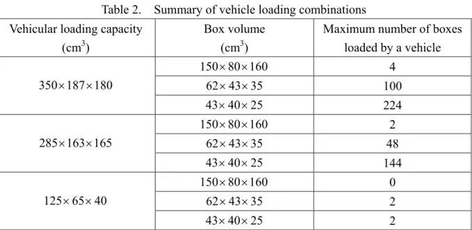
the loading capacity of 125×65×40 cm3. For convenience in the vehicular loading, three types of boxes used for loading products were utilized with volumes of 150×80×160 cm3 (large-size), 62×43×35 cm3 (medium-size), and 43×40×25 cm3 (small-size). The potential combinations of the aforementioned vehicular loading capacities and package volumes are summarized in Table 2. The original frequency of daily vehicle dispatch of the targeted logistics company was three times a day, departing from the corresponding warehouse at 9:00, 13:00, and 17:00, respectively. The dispatched fleet size in each delivery mission depended primarily on the volume of the ordered goods, but was subject to the maximum fleet size available. Herein, vehicular en-routing paths depended primarily on the experiences of the corresponding drivers and their responses to the present road traffic conditions.

Table 2. Summary of potential vehicle loading combinations

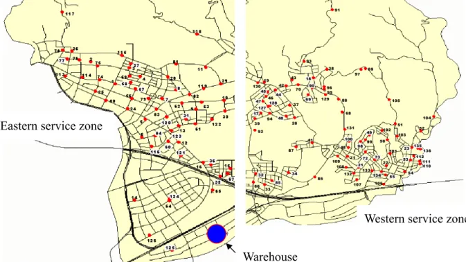
In order to generate a database used to illustrate the applicability of the proposed method, a total of 136 order entries scheduled to be served in a given 1-day testing period were selected as the input database following the order-processing criteria mentioned previously in the first phase of the proposed approach (see Eqs. (1) and (2)). The corresponding geographical relationships of these customers are depicted in Fig. 4, which graphically bounds these customers by two service zones (i.e., the eastern and western delivery service zones), consistent with the existing delivery service zones adopted by the targeted logistics company.

Fig. 4. Geographic distribution of customers

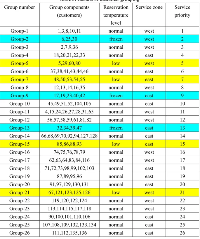
Following the second and third phases of the proposed logistics resource allocation system (i.e., customer grouping and ranking), the collected order entries have been reprocessed and then classified the customers into specific groups through the proposed

algorithms. The numerical results of customer grouping are summarized in Table 3, which also shows the clustered customer group numbers and service priority.

Table 3. Results of customer grouping

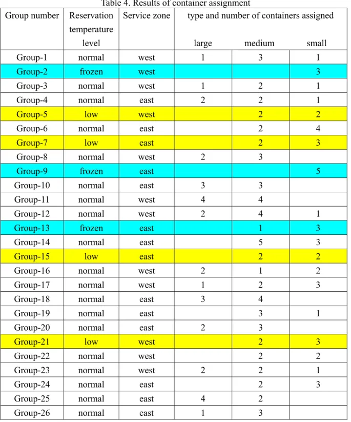
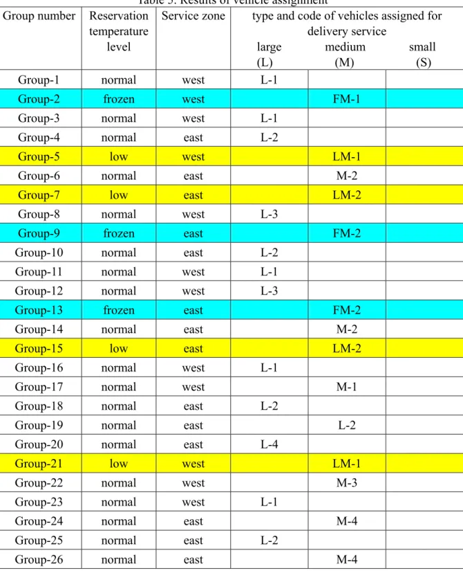
After the aforementioned customer grouping and ranking determination phases, the corresponding resource assignment mechanisms including container and vehicle assignments were conducted by following the procedures of phases 4 and 5 (i.e., container and vehicle assignment) of the proposed method. Here, the weights associated with the corresponding objective function of the container assignment phase (i.e., ϖ_CR and ϖ_PC shown in Eq. (15)) are tentatively set to be 0.5; and similarly, the weights introduced for the vehicle assignment (i.e., ϖ_VR, ϖ_OC and ϖ shown in Eq. (25)) are tentatively set to be 1/3 in this test _DT scenario. Nevertheless, the setting of these weights will be examined later in the following sensitivity analysis scenario to investigate their effects on system performance. The corresponding resource assignment results obtained in this scenario are summarized in Tables 4 and 5. Note that to simplify the structure of the real logistical distribution network, only major streets in the real network were considered in estimating the time-varying vehicular return possibility (σ(k)) mentioned in Eq. (36) to determine the fleet size of available vehicles at each given time step k.

Table 4. Results of container assignment

Table 5. Results of vehicle assignment

Obtained from the above numerical results, two generalizations can be made. First, among the three categories of normal-product freight vehicles, only large-sized and medium-sized vehicles are assigned under the condition that the delivered customer orders are

grouped using the proposed vehicle assignment model. In contrast, small-sized vehicles are used for short-distance and miscellaneous goods delivery services in the present delivery strategy. Second, through the procedures of dynamic customer order grouping and logistics resource assignment, different customer groups (e.g., customer groups 1 and 3 shown in Table 5) can be consolidated, and then served with the same vehicle without the need of efforts for extra vehicle loading and dispatching. Under such operational conditions, the groups of customer orders loaded in a given vehicle can be readily served in sequence in a given vehicle routing mission following the estimated group service priority.

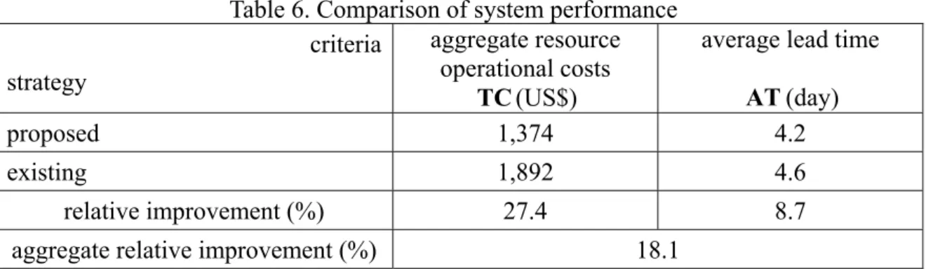
To quantitatively assess the relative performance of the proposed method with respect to the improvements in logistics resource utilization, we compared the operational results obtained from the proposed distribution strategy and the original strategy, using two major criteria defined in the following.

(1) TC, which represents the aggregate logistics resource operational costs spent in the given test period; and

(2) AT , which represents the average lead time associated with each given customer.

Here TC aims to sum up the corresponding internal logistics resource operational costs, including the packaging and loading costs associated with the corresponding resources as well as vehicle routing costs; and AT , in contrast, is measured by averaging the time difference

between when an order is received and when the loading of the corresponding goods is completed for all the sampled customers. Note that to facilitate the aforementioned model evaluation, only the static link costs are considered in estimating the corresponding vehicle routing costs of TC. The comparison results according to the aforementioned criteria are summarized in Table 6.

Overall, the results shown in Table 6 reveal that there is a certain improvement in the performance of logistical resource utilization using the proposed dynamic resource allocation methodology. Two supportive generalizations made according to the corresponding numerical results are summarized below.

First, as can be seen in Table 6, the relative improvement of the logistics system performance results mainly from the reduction in the aggregate logistics resource operational costs. Based on this numerical study, such a group-based vehicle dispatching coupled with appropriate resource assignment strategies can be beneficial in enhancing the efficiency of en-route goods delivery, thus contributing to a significant improvement in the corresponding operational costs as high as 27.4%.

Second, through appropriate pre-route customer classification and group-based logistics resource allocation strategies, grouped customers can be served more efficiently. The results presented in Tables 5 and 6 show that the resulting customer order grouping and vehicle assignment may contribute to greater vehicle dispatching frequency without extra time and costs in resource allocation. Accordingly, the corresponding group-based customer delivery services can be completed with shorter lead times, relative to the original delivery schedule, thus contributing to a relative improvement of 8.7% in terms of average lead time (AT ). To a certain extent, this implies that higher customer service quality can be achieved

using the proposed logistics resource allocation methodology.

In addition, several findings are summarized below for further discussion.

(1) Although the proposed logistics resource allocation method appears to satisfy customer demands for shorter lead time to a certain extent, timeliness may remain as a significant issue in time-based logistics control, requiring further investigation. For instance, to implement just-in-time (JIT) inventory control strategies, the major request from customers may no longer be shorter lead time, but the more exact goods delivery time.

Sometimes earlier goods delivery service may not be a benefit to those customers who implement JIT strategies due to the induced inventory costs in this case, and vice versa. (2) Despite the measurements of TC and AT , both indicating certain improvements in

logistics resource operational costs and service time, respectively, it is likely that the performance of logistical distribution operations can also be improved by integrating either advanced vehicle routing technologies or advanced ITS-related technologies, including global positioning systems (GPS) and two-way communication devices. (3) The measurements shown in Table 6 may also be beneficial in diagnosing the existing

logistics resource management performance of the targeted logistics company. Definitely, the comparison results imply that there is a potential to improve the current logistics resource allocation and vehicle dispatching strategies undertaken by the targeted logistics company. Such improvements can then enhance the customer service quality not only to the downstream end-customers but also to its upstream contracted manufacturer who also plays the role of a customer to the targeted logistics company.

Furthermore, it is worth mentioning that the computational efficiency could be another potential advantage of the proposed method. It has been observed that in the corresponding data processing and computational procedures, such a group-based logistics resource allocation methodology enables great time savings in algorithmic execution. For instance, as can be seen in Table 3, the maximum number of customers to be served in a given group is 8, which does not appear to be a burden in searching the optimal solutions for either logistics multi-resource allocation or the induced vehicle routing problems.

In the following test scenario, simple sensitivity analyses are conducted to demonstrate the generality of the numerical results. This test scenario mainly aims at two groups of parameters. The first group involves the weights presented in the proposed composite objective functions for container and vehicle assignment. The second group involves four

selected operational parameters, including the cluster threshold λ , the unit costs of ₂ packaging and vehicle operations (i.e., c and _jg d , respectively), and the expected delivery _lg

times associated with customer groups (st ). Here, _g λ is regarded as a clustering-oriented ₂

parameter which may influence the customer group number in the study; and the others are supply-oriented parameters that may have the effects on the operational performance of allocating containers and vehicles. The corresponding numerical results associated with these two groups of parameters are summarized in Tables 7 and 8, respectively, where all the results presented in these two Tables are relative improvements compared to the existing operational performance of the targeted logistics company. Conveniently, the aforementioned evaluation measures, i.e., TC and AT , remain used in this test scenario.

Here, all the preset parameters of the proposed method remain the same, except the targeted parameters.

Table 7. Results of sensitivity analyses with respect to weights

Based on the numerical results of Table 7, four major generalizations are summarized below.

(1) Compared to the weights associated with the container-assignment objective functions (i.e., ϖ_CR and ϖ_PC ), the weights associated with the vehicle-assignment objective functions (i.e., ϖ_VR, ϖ_OC, and ϖ ) appear to have relatively significant effects on the _DT improvement with respect either to the aggregate operational costs (TC) or to the average lead time (AT ). This implies that dynamic vehicle assignment coupled with

proper vehicle dispatching strategies play a key role in logistics resource allocation, and determine the performance of city logistics distribution operations.

(2) Relative to ϖ_CR, ϖ_PC seems to have a greater effect on the improvement of TC, as the value of ϖ_PC increases. In contrast, the increase of ϖ_CR merely has a slight effect on the improvement of AT , and meanwhile may not help to improve TC. (3) Among these targeted weights, ϖ_OC and ϖ may have more significant effects on _DT

the improvement of TC and AT , respectively. As can be seen in Table 7, under the

corresponding extreme cases (i.e, ϖ_OC =1 and ϖ_DT =1), the evaluation measures TC

and AT can be improved up to 32.7% and 15.2%, respectively, relative to the existing

operational performance.

(4) Following the above generalizations, it is induced that saving the operational costs by about US$144 may be equivalent to saving the lead time as high as 0.4 day (about 9.6 hour), compared to the aforementioned two extreme cases (i.e, the cases of ϖ_OC =1 and

1 =

DT

ϖ ). Correspondingly, the logistics company manager may need to sustain the extra costs of about US$15 to save 1 hour in terms of the average lead time for higher customer service quality. Accordingly, the logistics company manager can choose one of these two alternative strategies depending on the corresponding business operational goal.

Table 8. Results of sensitivity analyses with respect to operational parameters

The numerical results shown in Table 8 may reveal the following three generalizations. (1) An appropriate setting for the range of the clustering-oriented parameter λ is needed ₂

since it determines the number of customer order groups, which may further influence the performance of dynamic resource allocation with respect to both the aggregate operational costs and average lead time to customers. As can be seen in Table 8, when the value of λ increases by 40%, i.e., ₂ λ₂ =0.98, the induced greater number of

customer order groups does not lead to relatively better performance, compared to the original setting (i.e., λ₂ =0.7). Similarly, the decrease of λ by 40% may contribute ₂ to a fewer number of customer order groups; however it does not correspond to a positive effect on saving the aggregate operational costs. Overall, the value of λ set ₂ within the range between 0.5 and 0.7 may lead to a better performance in the study case. (2) Both the increments of the unit packaging and vehicle operational costs appear to merely

have the effects on the aggregate operational costs, and relatively, the induced effect associated with the unit vehicle operational cost appears to be greater than that of the unit packaging cost.

(3) The increments in the expected delivery times appear to have relatively greater effects on the average lead time than that on the aggregate operational costs. As can be seen in Table 8, the average lead time can be improved up to 13% when the expected delivery time associated with each given customer group is decreased by 40%. In contrast, the corresponding effects on the aggregate operational costs appear to be less significant in this study case.

In addition, from the above numerical results, three managerial implications are provided below.

First, the conduction of appropriate customer order grouping and resource assignment prior to vehicle dispatching do improve the performance of city logistics systems in reducing the operational costs and average lead time. Motivated by the above concept as well as the numerical results, logistics managers can integrate such sequential procedures proposed in this study with any existing logistics information systems to enhance the entire competitiveness of business operations in time-based logistics control.

Second, as revealed in the corresponding sensitivity analysis, the reduction of the expected delivery time associated with each customer group appears to have a significant

effect on stimulating the customer satisfaction with the improved average lead time. To achieve the above operational goal, the incorporation of novel route guidance technology with the proposed dynamic resource allocation method is needed.

Third, considering the diversity of customer demands exhibited in differing logistics distribution channels and the resulting complicated operational environments, the functionality of a dynamic logistics resource allocation system should be flexible enough to be adjusted. For instance, aiming at specific distribution channels and operational environments, respective customer attributes together with operational parameters can be specified, and then embedded in the proposed method for further practical uses without any extra effort in system reformulation.

Concluding remarks

This paper has presented a comprehensive system framework, including order processing, customer order grouping and ranking, container assignment and vehicle assignment, for dynamic logistics multi-resource allocation. Through analyzing customers’ order attributes, the proposed method executes the proposed hybrid hard-and-fuzzy clustering algorithms together with customer-group ranking logic rules to group customer orders by their delivery service priority, followed by operating the functions of container and vehicle assignment in response to the variety of grouped customer demands. In addition, the time-varying possibility of en-route vehicle returning is considered in formulating the proposed vehicle assignment model.

In order to demonstrate the potential advantages of the proposed method, numerical studies on the existing logistics resource allocation strategies of a targeted logistics company were conducted. By comparing the performance of the proposed logistics resource allocation method with that of the original strategies executed by the targeted logistics

company, the numerical results revealed that the overall logistics system performance could be improved by up to 27.4% and 8.7% in terms of the aggregate resource operational costs and average lead time, respectively. Furthermore, it is found that such improvement may mainly result from the proposed vehicle assignment model coupled with the appropriate customer grouping strategies in quick response to grouped customer orders. In addition, sensitivity analyses with respect to the corresponding weights of the objective functions and several key operational parameters were conducted and discussed.

Nevertheless, there may still be a great potential for either improving or expanding the proposed method by integrating more elaborate vehicle routing algorithms for quick-responsive logistics distribution operations. Such an integrated customer group-based logistics distribution operation appears important to provide efficient goods delivery service in a large-scale logistics network under time-varying traffic network conditions.

Furthermore, the case of crossover distribution based on product temperature may not be considered in the present study scope considering the differing lifecycles of products as well as packaging requirements. Nevertheless, we would also like to leave the door open for future research to deal specifically with the aforementioned crossover distribution case if the induced effects are allowable in practical applications. In that case, the corresponding clustering criterion, the required reservation temperature level, may no longer be needed, and the resulting improvements in system performance, particularly in terms of cost saving, as well as the induced effects may warrant more evaluation.

It is expected that the proposed dynamic logistics multi-resource allocation method can make benefits available not only for developing advanced logistics distribution strategies, but also for clarifying the importance of pre-route customer grouping in the operations of time-based logistics control and management. On the basis of the present results, our future research will aim at incorporating advanced vehicle routing and ITS-related technologies into

the architecture of the proposed method to improve the performance of time-based demand-responsive logistics distribution operations. Moreover, the applicability of the proposed method for logistics operations in more real e-business operational cases is also of interest to us, and warrants further research.

Acknowledgements

This research was supported by the grant NSC 93-2416-H-009-006 from the National Science Council of Taiwan. The author would also like to thank the referees for their helpful comments. The valuable suggestions of Professor Wayne K. Talley to improve this paper are also gratefully acknowledged. Any errors or omissions remain the sole responsibility of the authors.

References

Altinkemer, K., and Gavish, B., 1990. Heuristics for delivery problems with constraint error guarantees. Transportation Science 24, 294-297.

Ballou, R. H., 2002. Transport decisions. In: Ballou, R. H. (Ed.), Business Logistics Management. Prentice-Hall, Upper Saddle River, New Jersey, 185-242.

Beltrami, W., and Bodin, L., 1974. Networks and vehicle routing for municipal waste collection. Networks 4, 65-94.

Bezdek, J. C., 1973. Fuzzy mathematics in pattern classification. Ph.D. Thesis, Cornell University, USA.

Blumenfeld, D. E., Burns, L. D., Daganzo, C. F., Frick, M. C., and Hall, R. W., 1987. Reducing logistics costs at General Motors. Interface 17, 26-47.

Bramel, J, Simchi-Levi, D (Eds.), 1999. The logic of logistics. Springer, New York.

Bramel, J., and Simchi-Levi, D., 1995. A location based heuristic for general routing problems. Operations Research 43, 649-660.