嵌入式圖形處理器之繪圖程式高階耗能模型

國

立

交

通

大

學

資訊科學與工程研究所

碩

士

論

文

嵌 入 式 圖 形 處 理 器 之 繪 圖 程 式 高 階 耗 能 模 型

A Study on High-Level Energy Model of Embedded GPU

研 究 生：鍾宇安

指導教授：曹孝櫟 教授

嵌入式圖形處理器之繪圖程式高階耗能模型

A Study on High-Level Energy Model of Embedded GPU

研 究 生：鍾宇安 Student：Yu-An Chung

指導教授：曹孝櫟 Advisor：Shiao-Li Tsao

國 立 交 通 大 學

資 訊 科 學 與 工 程 研 究 所

碩 士 論 文

Submitted to Institute of Computer Science and Engineering College of Computer Science

National Chiao Tung University in partial Fulfillment of the Requirements

for the Degree of Master

in

Computer Science October 2014

Hsinchu, Taiwan, Republic of China

i

嵌入式圖形處理器之繪圖程式高階耗能模型

國立交通大學

資訊科學與工程研究所 碩士班

摘要

嵌入式圖型處理器可加速行動裝置上的繪圖程式之繪圖處理，但同時也

需消耗可觀的耗電[1]。由電池驅動的行動裝置之耗電量無疑是非常重要的。

為了能預估繪圖程式的耗電量，過去研究會去收集 GPU 硬體元件之計數器的

數值來作為耗能模型之參數並預測耗能。但這些參數無法協助繪圖工程師來

撰寫較省電之繪圖程式。為了讓繪圖工程師了解繪圖品質與耗能的關係，此

篇論文建立了一個只需要繪圖參數，不需要硬體計數器即可預測繪圖程是耗

能的耗能模型，以協助繪圖工程師在繪圖品質與耗能中取得一個平衡點。此

耗能模型的預估值與實際量測的耗能的誤差為 7.7%。

ii

A Study on High-Level Energy Model of Embedded

GPU

Student：Yu-An Chung Advisor：Shiao-Li Tsao

Institue of Computer Science and Engineering College of Computer Science

National Chiao Tung University

Abstract

Embedded graphic processing unit (GPU) accelerates a real-time rendering process of a graphics application on mobile devices, however, at the cost of consuming a considerable portion of the system energy [1] which is one of the most critical design issues for battery-operated devices. To estimate the power consumption of a graphics application, conventional approaches collect run-time hardware activities of a GPU, and derive the power consumption of the graphics application based on hardware counters. Unfortunately, these hardware counters and power consumption information are difficult to evaluate from a programmer's point of view. In order to provide graphics programmers a firm notion of how performance and quality relate to energy cost, a high-level power model to assist programmers to balance performance, quality, and energy budget is proposed in this study. The high-level power model only requires high-level graphics data to estimate the power consumption of a graphics program. The error rate of the model is around 7.7%.

iii

誌謝

首先我要謝謝我的指導教授: 曹孝櫟教授，從老師身上學到了很多東西，包

含研究的態度與方法。老師平常也用幽默的方式來教導我們、引導我們，讓我們

可以順利的完成研究。接著我要感謝我的口試委員，徐慰中教授、范倫達教授、

與張鈞法教授，他們給了我許多寶貴的建議讓這篇論文內容更加充實完善。

我也要謝謝實驗室的學長，建臻、承威和宇宸學長，在研究的路上有他們可

以請教和討論真的很幸運。除了和他們學習研究的方法之外，也學到了與人相處

應對的小技巧。此外也要感謝實驗室的同儕與學弟，和他們一起做計畫研究和分

享碩士生活、一起奮鬥，和大家一起相處真的非常愉快。

最後我要謝謝我的家人和培嘉，在背後支持我讓我可以專心做研究，也讓我

有可以靠岸休息的地方，有妳們的陪伴真的很溫暖。

iv

Table of Contents

4.1. Construction of a High-Level Power Model ... 8

4.2. High-Level Input Data ... 9

4.3. Hardware Counters... 10

5. Experiment ... 12

5.1. Experiment Setup ... 12

5.2. High-level to Hardware Counter ... 12

5.2.1. Vertex Shader ... 12

5.2.2. Tile Accelerator ... 13

5.2.3. Image Synthesis Processor... 14

5.2.4. Fragment Shader ... 15

5.3. Hardware Counter to Power Consumption ... 18

5.4. Validation ... 19

5.4.1. Vertex Shader ... 19

5.4.2. Tile Accelerator ... 19

5.4.3. Image Synthesis Processor... 20

5.4.4. Fragment Shader ... 21

5.4.5. Hardware Counter to Power Consumption ... 21

5.4.6. High-level Power Model ... 22

6. Conclusion ... 24

v

List of Figures

Figure 1. OpenGL pipeline ... 5

Figure 2. Immediate Mode Rendering (IMR) ... 6

Figure 3. Tile-based Deferred Rendering ... 6

Figure 4. Construction of High-Level Power Model ... 8

Figure 5. Stages of Power Model Construction ... 9

Figure 6. Input Data Flow of GPU ... 10

Figure 7. Vertex Shading Time ... 12

Figure 8. Baseline of TA under different Resolutions ... 13

Figure 9. TA time and # of Vertices under different vertex shaders ... 14

Figure 10. Relation of ISP time and # of Vertices after Clipping and Culling ... 15

Figure 11. Baseline of ISP under different Resolutions... 15

Figure 12. Baseline of Fragment Shader under different Resolutions ... 17

Figure 13. Fragment Shading time with Different Fragment Shader ... 17

Figure 14. Fragment time and # of Vertices under different fragment shaders ... 18

Figure 15. Vertex Time ... 19

Figure 16. TA Time ... 20

Figure 17. ISP Time ... 20

Figure 18. Fragment Time ... 21

Figure 19. Low-level Model Energy ... 22

vi

List of Tables

Table 1. High-level Inputs ... 10 Table 2. Number of Tiles for different Resolutions ... 10 Table 3. Hardware Performance Counters ... 11

1

1. Introduction

Due to high demands on graphics processing, graphic processing unit (GPU) in mobile devices has become an indispensable component. The GPU accelerates the rendering process of a graphics application, however, at the cost of consuming a considerable portion of the system energy [1]. In contrast to desktop developers, mobile device programmers have to strike a good balance between performance, quality, and power consumption in a battery-operated device. It is thus vital for graphics programmers to have a firm notion of how performance and quality relate to energy cost at the development stage.

Desktop GPUs and embedded GPUs are designed differently to suit their working condition and performance target. Desktop GPUs aim for high performance and do not have to worry about power supply. On the other hand, embedded GPUs operate in a battery-operated device and thus have to be designed with low-power consumption. Most of the contemporary embedded GPUs [2, 11, 12] are based on tile-based rendering design (partition the display into small rectangles) to reduce memory transfer energy consumption. Previous studies on GPU power model mainly focuses on desktop GPUs, without considering tile-based design and the associated micro-architecture changes. These design differences have to be considered in constructing an embedded GPU power model. Specifically, we focused on a state-of-the-art Tiled-Based Deferred Rendering (TBDR) architecture proposed by Imagination [2].

Embedded graphics programmers nowadays mainly use OpenGL [3] (OpenGL ES [4] for Embedded Systems) to control the GPU for rendering the scenes in real-time. Therefore we aim to analyze the power consumption behavior of the GPU executing a real-time OpenGL program. An OpenGL program mainly consists of data (such as mesh data, texture data, and camera position) and shader programs (such as vertex shader and fragment shader). Thus our main concept is to develop a micro-benchmark suites specifically tailored for mobile GPUs to systematically stress different pipeline stages (ex. submit lots of vertices to increase vertex shader’s loading or even generate pipeline stalls) and analyze the corresponding energy consumption behavior.

According to the analysis results, important parameters are chosen to build our high-level power model. Different from previous studies aiming at low-level hardware dependent desktop GPU power model [5], this research proposes a high-level power model of embedded GPUs from a programmers' perspective. With the proposed power model, graphics programmers will be better equipped with the knowledge about how their programs are being processed by the

2

embedded GPU and the associated energy cost during development time. With such a high-level power model, it is also possible to conduct a high-high-level resource management to balance between power, performance, and quality for real-time graphic rendering. In summary, the main contributions of this study are:

1. Developed a micro-benchmark suites specifically tailored to the mobile GPU design. 2. Constructed a high-level power model to assist graphics programmer to balance

between performance, quality, and energy budget.

The rest of the paper is organized as follows: In Section II, we give a brief summary on previous studies about GPU power models. In Section III, an introduction on the OpenGL pipeline and the architecture of an embedded GPU is given. In Section IV, we discuss the idea of our power model and experiment design. In Section V, the measurement environmental and preliminary experimental results will be shown. Finally, in Section VI, the conclusion and future work will be brought out.

3

2. Related Work

Previous research on the power consumption of GPU mostly focuses on desktop GPUs with comparatively less focus on embedded GPUs. Collange et al. [6] used an oscilloscope to measure the GPU energy consumption in a CUDA environment, to find out the bottleneck of a GPGPU program. Shaikh et al. [7] profiled the power consumption of two GPU architectures: GF100 and GT200. Their results show that the power dissipation of a data transfer instruction consumes less than half of that of a kernel instruction. Thus it is possible to identify which part of the program is running at a certain time. Ma et al. [5] chose five main GPU workload signals to build a power model, where the workload signals represent the runtime utilizations of the major pipeline stages on the GPU. They also compared the error rate between two different regression methods, namely Support Vector Regression (SVR) and Simple Linear Regression (SLR). The chosen SVR model outperformed the traditional SLR on their validation datasets. Hong and Kim [8] designed a set of micro-benchmarks to stress different architectural components of the GPU, and built not only the power model of the GPU but also the temperature model as well. They came out with the result: power consumption can be reduced by opening the appropriate number of streaming multiprocessors (SMs) in the GPU instead of using all the SMs. Leng et al. [9] built a power model for GPGPU using the power measurement data and performance counters from GPGPU-Sim, and also can estimate the GPU component's power consumption. They proposed a micro-benchmarking design methodology which includes the following: component stress, access patterns and test coverage. The above studies are all based on GPUs on desktop computers. Also, most of the above studies require hardware performance counters to estimate the power, which might not be easy to be interpreted by graphics programmers.

Following we list some studies related to mobile GPUs. Mochocki et al. [10] used three embedded processors to simulate different stages in the 3D pipeline. They analyzed how the factors (resolution, frame rate, level of detail, lighting model, and texture model) affect the 3D pipelines to result workload variations and imbalances. Moreover, DVFS was applied to processors to reduce the workload imbalance and can achieve up to 50% energy saving. Vatjus-Anttila et al. [1] built a power model based on three render complexity characteristics: number of triangles, render batches and addressed texels. Instead of measuring only the GPU's power consumption, the whole device's power consumption was used. To compensate the overestimated power, they empirically deducted 45% of the consumption based on the ad-hoc hypothesis that 50% of the 3D content could be left unacknowledged due to the back-face

4

triangle culling, and 10% due to depth testing. Mochocki et al. [10] studied about how some graphics factors affect the 3D pipelines, but they did not use a real embedded GPU for their experiments and neglected the architectural differences between desktop and embedded GPUs. Vatjus-Anttila et al. [1] built a power model for the whole embedded system based on render complexity. Our goal is to first understand the relation between high-level graphics parameters and the graphics pipelines. Then, we build a high-level power model for embedded GPU that only requires high-level parameters to estimate the power for real-time graphic rendering.

5

3. Background

3.1. OpenGL Pipeline

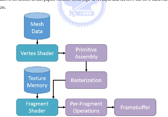
OpenGL is an API for advanced 3D graphics and it provides functionality to control the GPU, while OpenGL ES is specially targeted at handheld and embedded devices. The OpenGL graphics pipelines are shown in Figure 1. Mesh data are first sent to the GPU, then vertex shading is applied on each vertex with the given vertex shader program. Next, the shaded vertices are assembled into individual geometric primitives, and then be clipped and culled in the primitive assembly stage. In the rasterization phase, primitives are converted into fragments which are potential visible pixels and will be processed by the fragment shader later on. The fragment shader receives fragments from the rasterizer and either discard a non-visible fragment or generate a color for a visible fragment according to the given shader program. After the fragment shader, the per-fragment stage goes through a series of tests (scissor test, stencil and depth test and blending) and writes the resulting color into the frame buffer. In an OpenGL program, we provide some input, including mesh data, vertex and fragment shader program and texture data, etc. for the GPU. The GPU then takes all the information about the 3D objects and renders it on screen. In this paper, we alter those high-level input and see how the GPU hardware reacts.

6

3.2. Embedded GPU

Desktop GPUs and embedded GPUs are designed differently to suit their working condition and performance target. Desktop GPUs aim for high-performance whereas embedded GPUs target for low power.

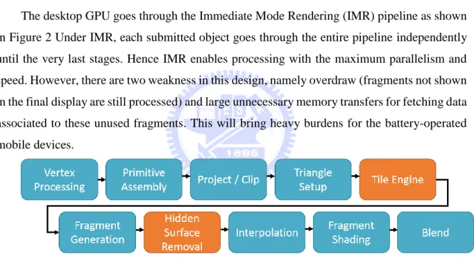
Figure 2. Immediate Mode Rendering (IMR)

The desktop GPU goes through the Immediate Mode Rendering (IMR) pipeline as shown in Figure 2 Under IMR, each submitted object goes through the entire pipeline independently until the very last stages. Hence IMR enables processing with the maximum parallelism and speed. However, there are two weakness in this design, namely overdraw (fragments not shown in the final display are still processed) and large unnecessary memory transfers for fetching data associated to these unused fragments. This will bring heavy burdens for the battery-operated mobile devices.

Figure 3. Tile-based Deferred Rendering

In order to solve these two critical issues, most of the contemporary embedded GPUs [2, 11, 12] adopt the tiling-based architecture. Since the data transfer between system memory and the GPU is one of the biggest cause for the power consumption of the GPU, tiling design claims to be able to reduce memory bandwidth requirement by partitioning the frame into small rectangles of pixels before rasterization. After coordinate transformation and triangle setup, the GPU determines tile-coverage of each triangle and records this information in a per-tile list. With this per-tile information, only relevant geometry data is needed when processing each tile in subsequent stages, therefore lowers the system memory bandwidth significantly. Imagination

7

PowerVR further adopts the Tile Based Deferred Rendering (TBDR) [2] pipeline as shown in Figure 3 to further reduce both overdraw and unnecessary memory transfers. We aim to verify the effectiveness of reducing overdraw and memory transfer of both TBDR and tiling-based designs in our study.

8

4. Methodology

4.1. Construction of a High-Level Power Model

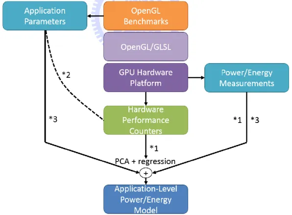
Previous studies on GPU power models [1] mostly focus on relating the power consumption to the hardware events by observing hardware performance counters of the GPU. A set of important hardware events such as memory transfer, cache misses, shader utilization, texture access, etc. were chosen and they are trained by a benchmark suite to build up the power model (*1 in Figure 4). This kind of power models are not very intuitive to graphics programmers since the programmers usually do not have a direct feeling about how their programs translate into hardware events. Our goal is to build a power model that can estimate power consumption with graphics related high-level parameters that programmers are familiar with (*2 in Figure 4). Using principal component analysis (PCA) [13] to select high-level parameters that are vital to the energy consumption, we can statistically relate the high-level parameters to GPU power consumption (*3 in Figure 4).

With this power model, programmers can have a better notion on how the GPU responds to their graphics program and can achieve a balance between performance, quality and energy.

Figure 4. Construction of High-Level Power Model

9

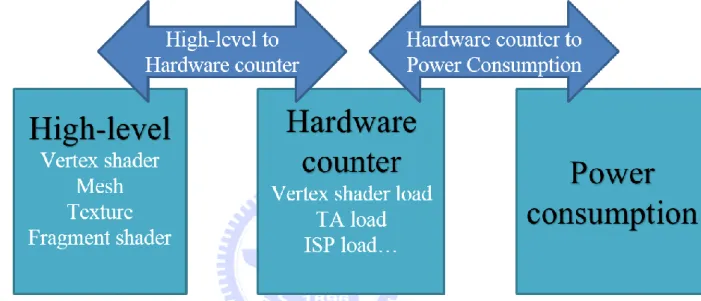
estimate the power consumption of an embedded GPU. And since power consumption is strongly related to the hardware components of the GPU. The first stage of the power model construction (Figure 5) is to find the mapping between high-level parameters and hardware counters. We will first build a high-level model to estimate the GPU’s hardware loading with the high-level parameters. The second stage of the power model construction is to use previously studied method to build a model to estimate power consumption by hardware counter values. After these two stages, it is possible to estimate power consumption without hardware counters but with only high-level parameters of a graphics program.

Figure 5. Stages of Power Model Construction

4.2. High-Level Input Data

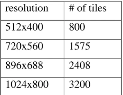
As mentioned in Section III, an OpenGL program receives a set of input data, including mesh data, texture data, vertex and fragment shader programs and some other control data. The data flow of the GPU is shown in Figure 6. A set of micro-benchmark is designed to change one different high-level input data at a time in order to figure out how each high-level input will affect the GPU’s hardware components. The list of high-level input data is listed in Table 1. Since the embedded GPU cuts the whole frame into small tiles (16x16 pixels) before processing it, we take the resolution into consideration as well. Table 2 shows the resolution and tiles relation.

10

Figure 6. Input Data Flow of GPU

High-level Input Affects Counts Mesh data # of vertices, # of triangles, percentage of

object hiding, # of visible fragments… 9 Vertex shader Lighting effect, vertex shader complexity… 13 Fragment shader Texturing, fragment shader complexity… 13 Resolution # of tiles 4

Table 1. High-level Inputs

resolution # of tiles 512x400 800 720x560 1575 896x688 2408 1024x800 3200

Table 2. Number of Tiles for different Resolutions

11

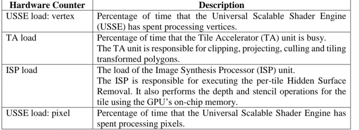
The description of the hardware performance counters we chose are listed in Table 2. These hardware counters are chosen because they represent the runtime utilizations of the major pipeline stages of the GPU. And therefore can be used to build the stage 2 model of the construction of the power model.

Hardware Counter Description

USSE load: vertex Percentage of time that the Universal Scalable Shader Engine (USSE) has spent processing vertices.

TA load Percentage of time that the Tile Accelerator (TA) unit is busy. The TA unit is responsible for clipping, projecting, culling and tiling transformed polygons.

ISP load The load of the Image Synthesis Processor (ISP) unit.

The ISP is responsible for executing the per-tile Hidden Surface Removal. It also performs the depth and stencil operations for the tile using the GPU’s on-chip memory.

USSE load: pixel Percentage of time that the Universal Scalable Shader Engine has spent processing pixels.

12

5. Experiment

5.1. Experiment Setup

The experiment environment is PandaBoard using the OMAP4430 processor with Imagination PowerVR SGX540 GPU [14]. Test programs are executed under Ubuntu 11.10 with a 3.1.0 Linux kernel using the OpenGL ES 2.0 library. Measurement of power consumption is done by using the TDS5032B oscilloscope to collect current data acquired by a current clamp through TCP A300[, with a sampling rate at 5K Hz.

5.2. High-level to Hardware Counter

5.2.1. Vertex Shader

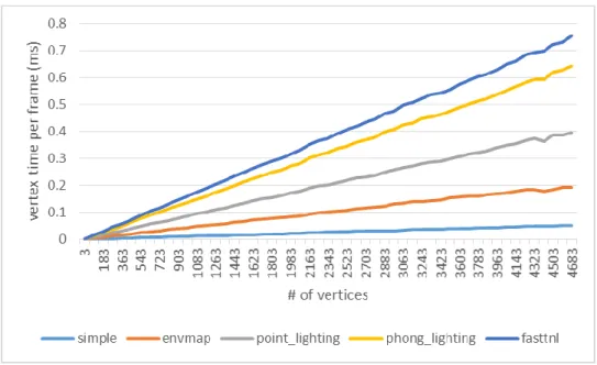
Figure 7. Vertex Shading Time

Figure 7 shows the relation between number of vertices and the time spent on vertex shading with different vertex shader programs. In the vertex shading stage, the vertex shader applies the vertex shader program onto each vertices, the result is easy to see. The time spent on vertex shading 𝑇𝑣𝑒𝑟𝑡𝑒𝑥 is shown in equation (1), where 𝑛𝑣𝑒𝑟𝑡𝑖𝑐𝑒𝑠 is the number of vertices

of the mesh data and 𝑊𝑣𝑒𝑟𝑡𝑖𝑥[𝑉] is the complexity of the given vertex shader program. And the

loading of the vertex shader component 𝐿𝑣𝑒𝑟𝑡𝑒𝑥 is shown in equation (2), where 𝑇𝑓𝑟𝑎𝑚𝑒 is the

time for drawing one frame.

𝑇𝑣𝑒𝑟𝑡𝑒𝑥 = 𝑛𝑣𝑒𝑟𝑡𝑖𝑐𝑒𝑠∗ 𝑊𝑣𝑒𝑟𝑡𝑖𝑥[𝑉]+ 𝐶𝑣𝑒𝑟𝑡𝑒𝑥 ( 1 )

13

5.2.2. Tile Accelerator

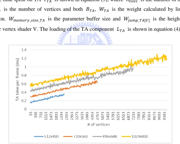
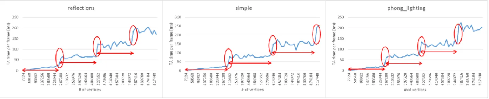
Figure 8 shows the relation between number of vertices and the time spent on TA. We can see that no matter under which resolution, the slope of the TA time remains the same. And also, there is a baseline for TA time even when there are no triangles submitted. It is easy to see that the baseline is related to the number of tiles. In Figure 9, we can see that when the number of vertices exceeds some value, there is a jump on the curve of TA time. Moreover, the number of vertices that will cause the jump and how high the jump is are different when different vertex shader program are applied in the previous vertex shading stage. The number of vertices that will trigger the jumps are 252840, 296184, 252840, and the height of the jumps are 35.6, 44.72, 40.68 (ms) accordingly when reflections, simple, and phong_lighing were applied for vertex shading.

The time spent on TA 𝑇_𝑇𝐴 is shown in equation (3), where 𝑛_{𝑡𝑖𝑙𝑒𝑠} is the number of tiles, 𝑛_{𝑣𝑒𝑟𝑡𝑖𝑐𝑒𝑠} is the number of vertices and both 𝐵_𝑇𝐴, 𝑊_𝑇𝐴 is the weight calculated by linear regression. 𝑊𝑚𝑒𝑚𝑜𝑟𝑦_𝑠𝑖𝑧𝑒_𝑇𝐴 is the parameter buffer size and 𝑊𝑗𝑢𝑚𝑝_𝑇𝐴[𝑉] is the height of

jump for vertex shader V. The loading of the TA component 𝐿𝑇𝐴 is shown in equation (4).

14

Figure 9. TA time and # of Vertices under different vertex shaders

𝑇_𝑇𝐴 = 𝑛_{𝑡𝑖𝑙𝑒𝑠}∗ 𝐵_𝑇𝐴+ 𝑛_{𝑣𝑒𝑟𝑡𝑖𝑐𝑒𝑠}∗ 𝑊_𝑇𝐴 + ⌊𝑛𝑣𝑒𝑟𝑡𝑖𝑐𝑒𝑠 ∗ 𝑊𝑣𝑒𝑟𝑡𝑒𝑥_𝑑𝑎𝑡𝑎[𝑉]

𝑊𝑚𝑒𝑚𝑜𝑟𝑦_𝑠𝑖𝑧𝑒_𝑇𝐴 ⌋ ∗ 𝑊𝑗𝑢𝑚𝑝_𝑇𝐴[𝑉] +

𝐶_𝑇𝐴 ( 3 )

𝐿_𝑇𝐴 = 𝑇_𝑇𝐴 ÷ 𝑇_{𝑓𝑟𝑎𝑚𝑒} ( 4 )

5.2.3. Image Synthesis Processor

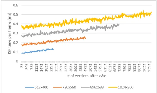
Figure 10 shows the relation between number of vertices after clipping and culling and the time spent on ISP. In the ISP stage, the ISP processes all the triangles and generates the fragments. And also calculates depth information to determine if the fragments are visible. As shown in Figure 11, there is a baseline for ISP even when there are no triangles submitted. And it is easy to see that the baseline is related to the number of tiles. The time spent on ISP 𝑇_𝐼𝑆𝑃 is shown in equation (5), where 𝑛_{𝑡𝑖𝑙𝑒𝑠} is the number of tiles, 𝑛_{𝑣𝑒𝑟𝑡𝑖𝑐𝑒𝑠𝑐𝑐} is the number of vertices after clipping and culling and both 𝐵𝐼𝑆𝑃, 𝑊𝐼𝑆𝑃 is the weight calculated by linear

15

Figure 10. Relation of ISP time and # of Vertices after Clipping and Culling

Figure 11. Baseline of ISP under different Resolutions

𝑇𝐼𝑆𝑃 = 𝑛𝑡𝑖𝑙𝑒𝑠∗ 𝐵𝐼𝑆𝑃+ 𝑛𝑣𝑒𝑟𝑡𝑖𝑐𝑒𝑐𝑐∗ 𝑊𝐼𝑆𝑃+ 𝐶𝐼𝑆𝑃 ( 5 )

𝐿_𝐼𝑆𝑃 = 𝑇_𝐼𝑆𝑃 ÷ 𝑇_{𝑓𝑟𝑎𝑚𝑒} ( 6 )

5.2.4. Fragment Shader

Figure 12 shows the relation between number of visible fragments and the time spent on fragment shading with different fragment shader programs. In the embedded GPU graphics

16

pipeline, before the fragments enter the fragment shading stage the ISP stage processes through all the fragments and compare their depth information to ensure that only fragments that will be rendered to screen are be submitted to the fragment shading stage. Therefore, the fragment shading is not related to number of vertices, but number of visible fragments instead. In the fragment shading stage, the given fragment shader is applied to each fragment to assign the final pixel color. As shown in Figire 12, given different fragment shaders, the slope of the fragment shading time differs.

Figure 13 shows the relation between number visible fragments and the time spent on fragment shading. We can see that no matter under which resolution, the slope of the fragment shading time remains the same. And also there is a baseline for fragment shading time even when there are no visible fragments. The baseline is related to the number of tiles.

In figure 14, we can see that when the number of vertices exceeds some value, there is a jump on the curve of TA time, which causes the fragment time to have a jump, too. Moreover, the height of the jump is different when different fragment shader program is applied. The number of vertices that will trigger the jumps are 209496, 166152, and the height of the jumps are 5.229, 2.138 (ms) accordingly when reflections, simple, and phong_lighing were applied for vertex shading.

The time spent on fragment shading 𝑇𝑓𝑟𝑎𝑔𝑚𝑒𝑛𝑡 is shown in equation (7), where 𝑛𝑡𝑖𝑙𝑒𝑠 is

the number of tiles, 𝑛𝑣𝑖𝑠𝑖𝑏𝑙𝑒_𝑓𝑟𝑎𝑔𝑚𝑒𝑛𝑡𝑠 is the number of visible fragments and both 𝐵𝑓𝑟𝑎𝑔𝑚𝑒𝑛𝑡,

𝑊𝑓𝑟𝑎𝑔𝑚𝑒𝑛𝑡 is the weight calculated by linear regression. 𝑊𝑗𝑢𝑚𝑝_𝑓𝑟𝑎𝑔𝑚𝑒𝑛𝑡[𝐹] is the height of

jump for fragment shader F. The loading of the fragment shader component 𝐿𝑓𝑟𝑎𝑔𝑚𝑒𝑛𝑡 is

17

Figure 12. Baseline of Fragment Shader under different Resolutions

18

Figure 14. Fragment time and # of Vertices under different fragment shaders

𝑇𝑓𝑟𝑎𝑔𝑚𝑒𝑛𝑡= 𝑛𝑡𝑖𝑙𝑒𝑠∗ 𝐵𝑓𝑟𝑎𝑔𝑚𝑒𝑛𝑡+ 𝑛𝑣𝑖𝑠𝑖𝑏𝑙𝑒𝑓𝑟𝑎𝑔𝑚𝑒𝑛𝑡𝑠 ∗ 𝑊𝑓𝑟𝑎𝑔𝑚𝑒𝑛𝑡[𝐹]+

⌊𝑛𝑣𝑒𝑟𝑡𝑖𝑐𝑒𝑠_𝑊 ∗ 𝑊𝑣𝑒𝑟𝑡𝑒𝑥𝑑𝑎𝑡𝑎[𝑉]

𝑚𝑒𝑚𝑜𝑟𝑦𝑠𝑖𝑧𝑒𝑇𝐴 ⌋ ∗ 𝑊𝑗𝑢𝑚𝑝_𝑓𝑟𝑎𝑔𝑚𝑒𝑛𝑡[𝐹]+ 𝐶𝑓𝑟𝑎𝑔𝑚𝑒𝑛𝑡 ( 7 )

𝐿_{𝑓𝑟𝑎𝑔𝑚𝑒𝑛𝑡} = 𝑇_{𝑓𝑟𝑎𝑔𝑚𝑒𝑛𝑡} ÷ 𝑇_{𝑓𝑟𝑎𝑚𝑒} ( 8 )

5.3. Hardware Counter to Power Consumption

The power consumption of the embedded GPU for one frame 𝑃_{𝑓𝑟𝑎𝑚𝑒} is shown in equation (9) and the energy consumption is shown in equation (14). When running through the micro-benchmarks, we record the hardware counter data and measure the power consumption. With the hardware loading data and power data, we use linear regression to retrieve the weight values (𝑊_𝑃𝑣𝑒𝑟𝑡𝑒𝑥, 𝑊_𝑃𝑇𝐴, 𝑊_𝑃𝐼𝑆𝑃, 𝑊_𝑃𝑓𝑟𝑎𝑔𝑚𝑒𝑛𝑡) of each component (𝑃𝑣𝑒𝑟𝑡𝑒𝑥, 𝑃𝑇𝐴, 𝑃𝐼𝑆𝑃,

𝑃_{𝑓𝑟𝑎𝑔𝑚𝑒𝑛𝑡}).

𝑃_{𝑓𝑟𝑎𝑚𝑒} = 𝑃_{𝑣𝑒𝑟𝑡𝑒𝑥}+ 𝑃_𝑇𝐴+ 𝑃_𝐼𝑆𝑃+ 𝑃_{𝑓𝑟𝑎𝑔𝑚𝑒𝑛𝑡}+ 𝐶_{𝑓𝑟𝑎𝑚𝑒} ( 9 ) 𝑃_{𝑣𝑒𝑟𝑡𝑒𝑥} = 𝐿_{𝑣𝑒𝑟𝑡𝑒𝑥}∗ 𝑊_𝑃_{𝑣𝑒𝑟𝑡𝑒𝑥} ( 10 ) 𝑃𝑇𝐴 = 𝐿𝑇𝐴 ∗ 𝑊_𝑃𝑇𝐴 ( 11 )

19

𝑃_𝐼𝑆𝑃 = 𝐿_𝐼𝑆𝑃 ∗ 𝑊_𝑃_𝐼𝑆𝑃 ( 12 ) 𝑃𝑓𝑟𝑎𝑔𝑚𝑒𝑛𝑡 = 𝐿𝑓𝑟𝑎𝑔𝑚𝑒𝑛𝑡∗ 𝑊_𝑃𝑓𝑟𝑎𝑔𝑚𝑒𝑛𝑡 ( 13 )

𝐸𝑓𝑟𝑎𝑚𝑒 = 𝑃𝑓𝑟𝑎𝑚𝑒∗ 𝑇𝑓𝑟𝑎𝑚𝑒 ( 14 )

5.4. Validation

After the model is trained and built with our micro-benchmarks, we use the test programs in the PowerVR SDK to validate the results.

5.4.1. Vertex Shader

Figure 15. Vertex Time

For the Vertex Shader part, measured and estimated 𝑇_{𝑣𝑒𝑟𝑡𝑒𝑥} are shown in Figure 15. The error rate ranges from 23.28% to 33.27%, and with an average error rate of 28.28%.

20

Figure 16. TA Time

For the Tile Accelerator part, measured and estimated 𝑇_𝑇𝐴 are shown in Figure 16. The error rate ranges from 2.95% to 9.96%, and with an average error rate of 6.80%.

5.4.3. Image Synthesis Processor

21

For the Image Synthesis Processor part, measured and estimated 𝑇𝐼𝑆𝑃 are shown in Figure

17. The error rate ranges from 5.65% to 16.74%, and with an average error rate of 11.09%.

5.4.4. Fragment Shader

Figure 18. Fragment Time

For the Fragment Shader part, measured and estimated 𝑇_{𝑓𝑟𝑎𝑔𝑚𝑒𝑛𝑡} are shown in Figure 18. The error rate ranges from 4.58% to 35.52%, and with an average error rate of 12.84%.

22

Figure 19. Low-level Model Energy

In section 5.3, we built a low-level power model with the measured hardware counter and power data from our micro-benchmarks. This model takes hardware counters as input and generates the power consumption. Here we show the error rate of the low-level power model. The measured and estimated 𝐸_{𝑓𝑟𝑎𝑚𝑒} are shown in Figure 19. The error rate ranges from 0.70% to 5.13%, and with an average error rate of 3.48%.

23

Figure 20. High-level Model Energy

Lastly, here is the validation for the high-level power model. This model only needs to take high-level graphics data as input to estimate the power consumption. The measured and estimated 𝐸_{𝑓𝑟𝑎𝑚𝑒} are shown in Figure 20. The error rate ranges from 6.24% to 10.45%, and with an average error rate of 7.71%.

24

6. Conclusion

In this study, a power model for embedded GPU that only requires high-level graphics input to estimate power is built. The power model is specially designed to fit in the architecture of an embedded GPU, therefore we can see how the model deals with tiling and HSR in this study. The validation part shows that the error rate of the model is 7.71%. With this power model, graphics programmers can have a basic concept on how the GPU reacts with different kind of graphics programs and therefore makes it possible to apply high-level power management in the future.

25

7. References

[1] J. M. Vatjus-Anttila, T. Koskela, and S. Hickey, “Power Consumption Model of a

Mobile GPU Based on Rendering Complexity,” in Proceedings of the 2013

Seventh International Conference on Next Generation Mobile Apps, Services and Technologies, Washington, DC, USA, 2013, pp. 210–215.

[2] ImaginationTechnologies Ltd, “PowerVR Series 5 Architecture Guide for

Developers.” 2014.

[3] D. Shreiner, G. Sellers, J. M. Kessenich, and B. M. Licea-Kane, OpenGL

Programming Guide: The Official Guide to Learning OpenGL, Version 4.3, 8th

ed. Addison-Wesley Professional, 2013.

[4] A. Munshi, D. Ginsburg, and D. Shreiner, OpenGL(R) ES 2.0 Programming Guide, 1st ed. Addison-Wesley Professional, 2008.

[5] X. Ma, M. Dong, L. Zhong, and Z. Deng, “Statistical Power Consumption Analysis

and Modeling for GPU-based Computing,” in Proc. of ACM SOSP Workshop on

Power Aware Computing and Systems (HotPower), 2009.

[6] S. Collange, D. Defour, and A. Tisserand, “Power Consumption of GPUs from a

Software Perspective,” in Proceedings of the 9th International Conference on

Computational Science: Part I, Berlin, Heidelberg, 2009, pp. 914–923.

[7] M. Z. Shaikh, M. Gregoire, W. Li, M. Wroblewski, and S. Simon, “In Situ Power

Analysis of General Purpose Graphical Processing Units,” in Proceedings of the

2011 19th International Euromicro Conference on Parallel, Distributed and Network-Based Processing, Washington, DC, USA, 2011, pp. 40–44.

[8] S. Hong and H. Kim, “An Integrated GPU Power and Performance Model,” in Proceedings of the 37th Annual International Symposium on Computer Architecture, New York, NY, USA, 2010, pp. 280–289.

[9] J. Leng, T. Hetherington, A. ElTantawy, S. Gilani, N. S. Kim, T. M. Aamodt, and V. J. Reddi, “GPUWattch: Enabling Energy Optimizations in GPGPUs,” in Proceedings of the 40th Annual International Symposium on Computer Architecture, New York, NY, USA, 2013, pp. 487–498.

[10] B. Mochocki, K. Lahiri, and S. Cadambi, “Power Analysis of Mobile 3D Graphics,” in Proceedings of the Conference on Design, Automation and Test in Europe: Proceedings, 3001 Leuven, Belgium, Belgium, 2006, pp. 502–507.

26

[12] Rob Clark, “Adreno tiling.” Internet:

https://github.com/freedreno/freedreno/wiki/Adreno-tiling, Apr-2014.

[13] I. T. Jolliffe, Principal Component Analysis. New York: Springer Verlag, 2002. [14] PandaBoard: http://pandaboard.org/