國 立 交 通 大 學
機 械 工 程 學 系
博 士 論 文
脈衝式電源驅動之平板型常壓氮氣為主介電質
電漿的流體模型模擬
Fluid Modeling of Parallel-plate Nitrogen-based
Dielectric Barrier Discharge Driven by a
Realistic Distorted Sinusoidal AC Power Source
研 究 生:鄭凱文
指導教授:吳宗信 博士
脈衝式電源驅動之平板型常壓氮氣為主介電質
電漿的流體模型模擬
Fluid Modeling of Parallel-plate Nitrogen-based
Dielectric Barrier Discharge Driven by a
Realistic Distorted Sinusoidal AC Power Source
研 究 生:鄭凱文
Student:Kai-Wen Cheng
指導教授:吳宗信 博士
Advisor:
Dr. Jong-Shinn Wu
國立交通大學
機械工程學系
博 士 論 文
A Thesis
Submitted to Department of Mechanical Engineering
College of Engineering
National Chiao Tung University
in Partial Fulfillment of the Requirements
for the Degree of
Doctor of Philosophy
In
Mechanical Engineering
July 2012
Hsinchu, Taiwan
西 元 2012 年 7 月
脈衝式電源驅動之平板型常壓氮氣為主介電質電漿的流體模型模擬
學生: 鄭凱文
指導教授: 吳宗信 博士
交通大學 機械工程學系
摘要
本論文考慮在交流 60 kHz 頻率的條件下,使用流體模型模擬脈衝式電源之 平板型氮氣為主的介電質電漿。從數值模擬計算出的電流-電壓曲線,發現在計 量上與實驗量測相當符合。 在純氮氣的數值模擬中,可看到 N4+離子為電漿濃度最高的帶電粒子。另外 改變介電質之間的距離超過 1.0 mm 時,氮氣電漿會從 Townsend-like discharge 轉變成 filamentary-like discharge 型式。實驗量測上也發現同樣的轉變現象。當 增加輸入的電壓時,電漿密度與電漿內部吸收的能量也隨之增加。由結果可看到 N4+離子獲得最多的能量並且超過電子吸收的十倍以上。介電質材質分析中,介 電值壁面上的累積電荷正比於介電常數。由於累積電荷越多,可提供越多離子化 時需要的電子,因此較容易維持電漿。另外增加介電質的厚度時對電漿密度與內 部能量吸收也有相當大的影響。 當微量的氧氣加入氮氣電漿時,可看到 N4+與 O2-離子有相同的密度且為電 漿濃度最高的帶電粒子。另外發現中性粒子 N2(A3Σ u+)與氮原子的模擬結果與實 驗量測非常相近。由於電子會大量吸附在氧氣上,降低電漿內部的電子密度,而 使電漿離子化的機率降低。因此可發現隨著氧氣濃度從 0.003 %增加到 0.1 %時, 電子的密度從 1017 m-3減少到 1014 m-3,並且發現只要加入少量的氧氣就會明顯 影響電漿的維持。在光譜的模擬結果上,選擇 second positive system (SPS)、NOγ-system 與 ON2-excimer 三組光譜與實驗量測作比較。兩者比較結果皆隨著氧 氣含量的增加,光譜強度從快速的增加轉變成逐漸的降低。
Fluid Modeling of Parallel-plate Nitrogen-based Dielectric Barrier
Discharge Driven by a Realistic Distorted Sinusoidal AC Power
Source
Student: Cheng, Kai-Wen Advisor: Dr. Wu, Jong-Shinn
Department of Mechanical Engineering
National Chiao-Tung University
Abstract
A simulation of parallel-plate dielectric barrier discharge (DBD) using pure nitrogen and N2/O2 gas driven by a realistic distorted-sinusoidal voltage power source
(60 kHz) is studied. The simulated current-voltage characteristic results quantitatively agree with experimental measurements.
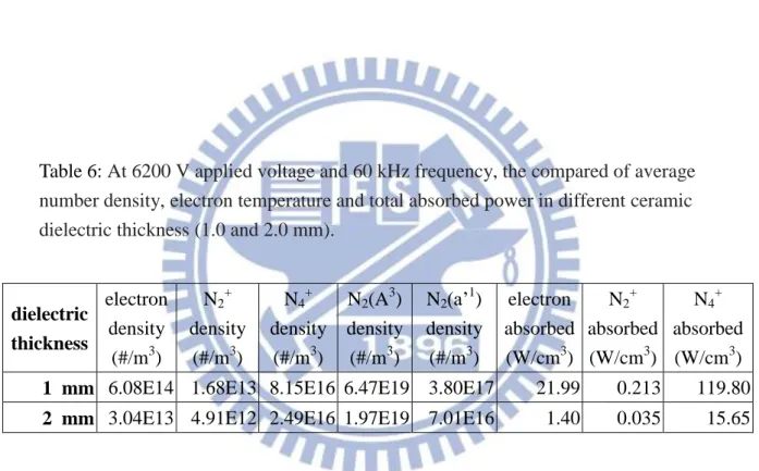
In the pure nitrogen simulations, N4+ ion density is the dominant charged species, which is unlike most glow discharges. The discharge transforms from Townsend-like to filamentary-like (microdischarge) as gap distance is more than 1.0 mm, which was also observed in the experiment. All densities of charged and neutral species increase exponentially with increasing applied peak voltages in the range of 6.2-8.6 kV. The higher permittivity of the dielectric material is, the larger the discharge current and the longer the period of gas breakdown are. In addition, the quantity of accumulated charge at each electrode increases with increasing permittivity of the dielectric material. Finally, the increase of dielectric thickness from 1.0 to 2.0 mm greatly reduces the densities of all species and also the plasma absorbed power.
When trace amount of oxygen is introduced in nitrogen plasma, the dominate charged species are N4+ and O2- with densities about 1018 m-3. The neutral species
densities of 2( 3 )
u
A
N and atomic nitrogen are approximately 4 × 10¹⁹ m-3 and 1 × 10²¹ m-3 respectively, which agree well with experiments. The oxygen addition can significantly decrease the electron density from the order of 1017 m-3 down to 1014 m-3 as the fraction of trace oxygen increases from 0.003 % to 0.1 %. In addition, the calculated photon radiations are compared against the measured spectra. The spectral bands of second positive system (SPS) of N2, NOγ-system and ON2-excimer are selected for comparison. Results reveal that the simulations and experiments show the similar trend with oxygen addition, in which the quantity of radiation increases rapidly first, peaks at some oxygen addition and then followed by a slow decrease.
致 謝
在交大的求學過程,誠摯的感謝吳宗信教授在這幾年的諄諄教誨,您對學 術的嚴謹和熱誠帶領著我們前進,並不時的為我們指引方向,在生活上非常照 顧我們,在學習和生活上讓我獲益良多。同時也要感謝口試委員陳慶耀老師、 徐振哲老師、魏大欽老師和陳彥升博士,謝謝您們在口試時提供的寶貴建議。另 外特別感謝學長粲哥,不僅付出時間和心力教導我研究上的問題,同時也在我 遇到許多困難時,給予我幫助與建議。 感謝實驗室的學長姐們,允民哥、周學姊、哲維兄、富利學長,也感謝實 驗室的夥伴們,邱哥、阿孟、昆哥、江學長、雅茹、正勤兄、豪哥、古必、楊宜 偉、劉志東、賴冠融、邱垂青、芳安、明忠等,與你們在一起相處的點點滴滴, 一起在實驗室努力的時光,是我一生最寶貴的回憶。也感謝學弟妹們的大力幫 忙,另外還有許多在生活或是學業上幫助我的人們或被不小心遺忘的朋友,在 此也一併感謝,並祝福所有我的朋友們,能夠達到自己理想的目標。 最後要特別感謝我的家人,尤其是老爸與老媽,在我的求學生涯中從未間 斷支持,這博士學位是父母親的成就。感謝他們對我的鼓勵與包容,在人生的 旅途上我會更加努力向目標邁進。 鄭凱文 謹誌 2012 年 7 月於交通大學Table of Contents
摘要 ... III Abstract ... V 致 謝 ... VII Table of Contents ... VIII List of Tables ... X List of Figures ... XI Nomenclature ... XIII
Chapter 1 Introduction ... 1
1.1 Background and Motivation ... 1
1.1.1 Characteristics of the Plasma ... 1
1.1.1.1 Definition of Plasmas ... 1
1.1.1.2 Type of Plasmas ... 1
1.1.1.3 Applications of Plasmas ... 2
1.1.2 Characteristics of the Atmospheric Pressure Glow Discharge... 3
1.1.3 Features of the Dielectric-Barrier Discharges (DBD) ... 4
1.1.3.1 Structures ... 4
1.1.3.2 Advantages ... 4
1.1.3.3 Applications ... 5
1.2 Literature Survey ... 5
1.2.1 Atmospheric Pressure Dielectric-barrier Discharges ... 5
1.2.2 Simulations and Experiments on DBD with Pure Nitrogen ... 6
1.2.3 Simulations and Experiments on DBD with Nitrogen Mixed Oxygen ... 7
1.2.4 Numerical Approaches for Plasma Simulation ... 8
1.3 Specific Objectives of the Thesis ... 9
Chapter 2 Research Methods ... 11
2.1 Numerical Method of Fluid Modeling ... 11
2.1.1 Boltzmann Equation ... 11
2.1.2 Fluid Modeling Equations ... 12
2.2 Implementation of Semi-Implicit Scheme ... 15
2.4 Numerical Algorithm ... 21
2.5 Experimental Methods ... 22
2.6 Kinetic Model ... 23
Chapter 3 One-Dimensional Simulation of Nitrogen Dielectric Barrier Discharge Driven by a Quasi-pulsed Power Source and Its Comparison with Experiments ... 26
3.1 Verification of the Fluid Modeling and Kinetic Model ... 26
3.2 Simulation Conditions ... 26
3.3 Basic Discharge Structure ... 27
3.4 Effect of Gap Distance ... 29
3.5 Effect of External Driving Voltage ... 30
3.6 Effect of Dielectric Material ... 31
3.7 Effect of Dielectric Thickness ... 32
Chapter 4 Numerical Investigation of Effects of Oxygen Addition on a Nitrogen-based Dielectric Barrier Discharge and Its Comparison with Experiments . 33 4.1 Simulation Conditions ... 33
4.2 Basic Discharge Structure ... 33
4.4 Influence of Trace Oxygen on Cycle Average Properties ... 35
4.5 Influence of Trace Oxygen on Spectroscopic Properties ... 36
Chapter 5 Conclusion and Recommendations of Future Work ... 37
5.1 Summary Remarks ... 37
5.2 Summary of Pure Nitrogen DBD Plasma ... 37
5.3 Summary of N2/O2 DBD Plasma ... 38
5.4 Recommendations of Future Work ... 39
References ... 40
List of Tables
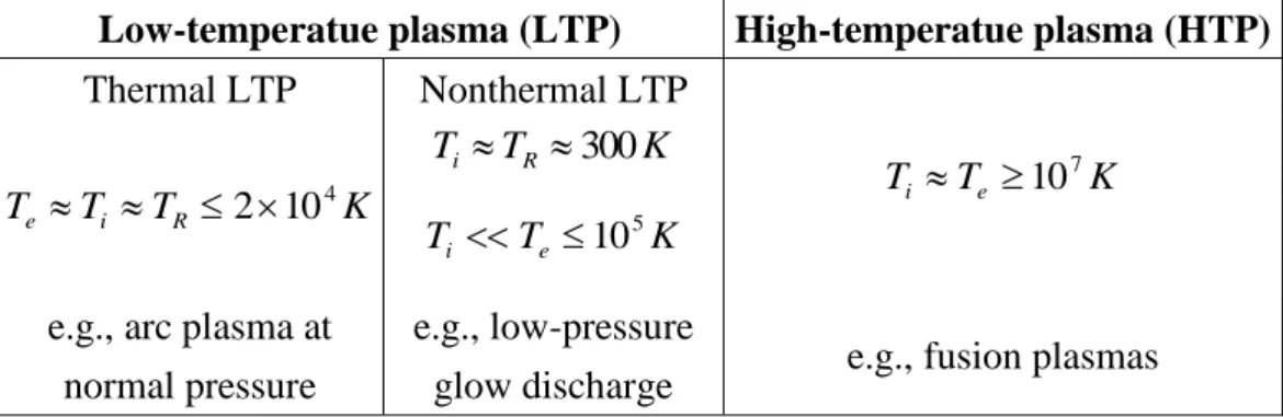
Table 1: Subdivision of plasmas ... 44
Table 2: Nitrogen Plasma Chemistry ... 45
Table 3: N2/O2 Plasma Chemistry ... 47
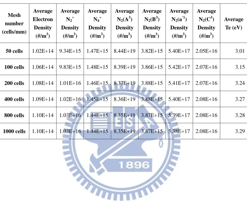
Table 4: Cycle average in different mesh number test ... 51
Table 5: Comparison of average absorbed power for varying applied voltage of 6200, 6600, 6800, 8600 V in a 60 kHz cycle, and a fixed gap distance of 0.5 mm. 52 Table 6: At 6200 V applied voltage and 60 kHz frequency, the compared of average number density, electron temperature and total absorbed power in different ceramic dielectric thickness (1.0 and 2.0 mm). ... 52
List of Figures
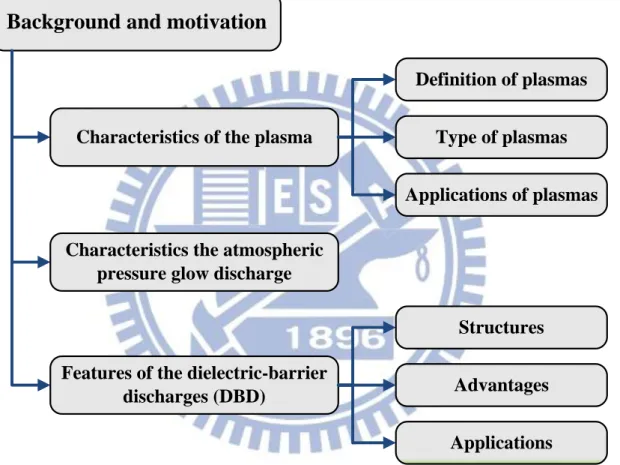
Figure 1. 1: The frame work of background and motivation ... 53
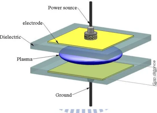
Figure 1. 2: Sketch of dielectric barrier discharge ... 54
Figure 1. 3: The frame work of literature survey ... 55
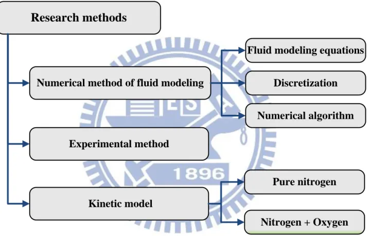
Figure 2. 1: The frame work of research methods ... 56
Figure 2. 2: The flowchart of plasma fluid modeling ... 57
Figure 2. 3: Schematic sketch of a planar DBD APPJ ... 58
Figure 3. 1: The frame work of pure nitrogen results and discussions ... 59
Figure 3. 2: Comparison of simulated (upper) and [Gherardi’s et al., 2001] experimental (bottom) voltages and currents for atmospheric pressure discharge using sinusoidal 8 kHz power source. ... 60
Figure 3. 3: Comparison of simulated and experimented current-voltage characteristic with voltage 6600 V and frequency 60 kHz. The distance between the two dielectric layers is 0.5 mm and the dielectric is 2.0 mm alumina. The photo image of discharge acquired by 0.2 second exposed time was at the right. ... 61
Figure 3. 4: Distributions of various discharge currents during a cycle via numerical modeling. The gap distance is 0.5 mm and using 2.0 mm thickness alumina dielectric. The applied voltage is 6600 V and 60 kHz frequency. ... 62
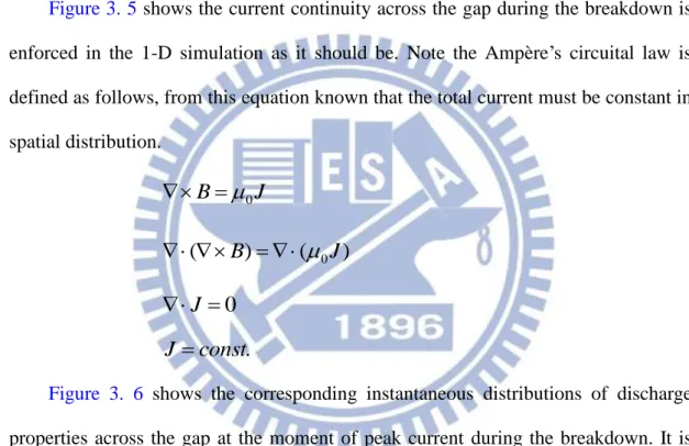
Figure 3. 5: Distributions of various discharge currents at the maximum discharge current via numerical modeling. The gap distance is 0.5 mm and using 2.0 mm thickness alumina dielectric. The applied voltage is 6600 V and 60 kHz frequency. ... 63
Figure 3. 6: Spatial distributions of electric field, charged particles and electron energy density at the time of maximum discharge current (0.86 μs) between two alumina dielectric. The operating conditions are the same as in Figure 3. 3. ... 64
Figure 3. 7: Spatial distributions of electric field, charged particles and electron energy density at 15.5 μs (after the breakdown) between two alumina dielectric. The operating conditions are the same as in Figure 3. 2. ... 65
Figure 3. 8: Comparison of different gap distance (a) 0.5 mm (b) 0.7 mm (c) 1.0 mm (d) 1.4 mm discharged currents along with photo images of discharge at the right. ... 66 Figure 3. 9: Cycle-space averaged number densities of various species in nitrogen
fixed gap distance of 0.5 mm. The alumina dielectric thickness is 2.0 mm and frequency is 60 kHz for all cases. ... 67 Figure 3. 10: Simulated current, gap voltage, applied voltage and accumulated charges at dielectric surfaces using 2.0 mm ceramic. The applied peak voltage is 8600 V and frequency is 60 kHz. The gap distance between dielectric is kept 0.5 mm. ... 68 Figure 3. 11: Simulated current, gap voltage, applied voltage and accumulated charges
at dielectric surfaces using 2.0 mm quartz. The applied peak voltage is 8600 V and frequency is 60 kHz. The gap distance between dielectric is kept 0.5 mm. ... 69 Figure 4. 1: The frame work of oxygen addition on nitrogen-based results and
discussions ... 70 Figure 4. 2: Comparison of simulated and experimented of N2 with 0.03% O2
current-voltage characteristic with voltage 8200 V and frequency 60 kHz. The distance between the two dielectric layers is 1.0 mm and the
dielectric is 1.0 mm quartz. ... 71 Figure 4. 3: Distributions of various spatial-average densities for charge species in N2
+ 0.03% O2 DBD. The applied peak voltage is 8200 V and frequency is 60 kHz. The gap distance between quartz dielectric is 1.0 mm. ... 72 Figure 4. 4: Distributions of various spatial-average densities for neutral species in N2
+ 0.03% O2 DBD. The applied peak voltage is 8200 V and frequency is 60 kHz. The gap distance between quartz dielectric is 1.0 mm. ... 73 Figure 4. 5: Cycle-space averaged number densities of various admixtures of oxygen
(from 0.003% to 0.1%) in nitrogen DBD, and a fixed gap distance of 1.0 mm. The quartz dielectric thickness is 1.0 mm and frequency is 60 kHz for all cases. ... 74 Figure 4. 6: The calculated radiations (full curves) and experimental optical emission
spectrums (dashed curves) were compared as a function of the trace oxygen. The spectral bands of SPS of N2, NOγ-system and ON2-excimer were selected. ... 75
Nomenclature
m massP pressure
q charge
B
k the Boltzmann constant
n number density
l thickness of dielectric barrier
L gap size of discharge region
particle flux
th
v thermal velocity
factor of secondary electron emission S source and sink of continuity equation Te electron temperature
energy loss for inelastic electron collision
potential 0 vacuum permittivity d dielectric permittivity E electric field
f electron energy distribution function
cross section
k reaction rate coefficient
mobility
D diffusivity
m
momentum exchange collision frequency between electron and background neutral particles
polarizability x space interval t time interval B Bernoulli function
Chapter 1 Introduction
1.1 Background and Motivation
A frame work of the background and motivation is revealed in Figure 1. 1. Three
categories of basic concept for plasma are introduced: characteristics of the plasma, characteristics of the atmospheric pressure glow discharge and features of the
dielectric-barrier discharges.
1.1.1 Characteristics of the Plasma
The term "plasma" was coined by Irving Langmuir in 1928, who was the
pioneers in gas discharges and defined plasma to be a region containing balanced charges of ions and electrons not influenced by its boundaries.
1.1.1.1 Definition of Plasmas
The plasma state is often referred to as the fourth state of matter. It is distinct from other lower-energy states of matter; most commonly solid, liquid, and gas. Much
of the visible matter in the universe is in the plasma state.
A plasma is a collection of free charged particles moving in random directions
that is, on the average, electrically neutral. Plasmas are ionized gases. Hence, they consist of positive (and negative) ions and electrons, as well as neutral species. The
ionization degree can vary from 100% (fully ionized gases) to very low values (e.g. 1e-4~1e-6; partially ionized gases).
1.1.1.2 Type of Plasmas
high-temperature plasmas and the so-called low-temperature plasmas. Further, based
on the relative temperatures of the electrons, ions and neutrals, low-temperature plasmas are classified as "thermal" or "non-thermal". Thermal plasmas have electrons
and the heavy particles at the same temperature, i.e., they are in thermal equilibrium with each other. Non-thermal plasmas on the other hand have the ions and neutrals at
a much lower temperature. Because of the large difference in mass, the electrons come to thermodynamic equilibrium amongst themselves much faster than they come
into equilibrium with the ions or neutral atoms. For this reason, the "ion temperature" may be very different from (usually lower than) the "electron temperature". This is
especially common in weakly ionized technological plasmas, where the ions are often near the ambient temperature.
1.1.1.3 Applications of Plasmas
Plasmas have been utilized in many well-established industrial applications (e.g. for surface modification, lasers, lighting, among others). In the following, we will
describe some of the most widespread applications:
First, surface treatment and modification with the possibility to treat (and to coat)
a surface at low temperature and at pressure close to atmospheric is an important advantage for industrial applications. The operating gases included air, He, N2, N2 + O2, Ar, CF4, NH3, Cl2, etc. Second, ozone is a potent germicide and one of the strongest known oxidants. The main applications of ozone generation are in water
treatment (drinking water plants using ozone for disinfection) and in pulp bleaching. The operating gases include dried clean air or dry oxygen. Third, plasma is used to
provide reactive species such as N2*, O2*, O(1D), O(3P), N(4S) in pollution control applications. These species initially formed by electron collisions in the
additional O and OH. These radicals can subsequently react with hazardous
compounds to form non-hazardous or less hazardous substances such as O2, O3, CO, CO2, H2O2. Fourth, gas discharges are also used for laser applications, more specifically as gas lasers (e.g. high speed welding and cutting of metal plates and other materials is the main application of silent discharge CO2 laser). Fifth, The
lamps especially used for high-speed printing on heat sensitive substrates. Large numbers of xenon excimer lamps are now routinely used for ‘‘UV cleaning’’ of
substrates in display and semiconductor manufacturing. Finally, plasma display panels (PDPs) displays utilizing Xe VUV radiation to excite phosphors are the most
recent addition to dielectric-barrier discharge applications.
1.1.2 Characteristics of the Atmospheric Pressure Glow Discharge
When the applied voltage exceeds the breakdown strength of the ambient gas, anavalanche is formed. During the short breakdown period, the non-conducting gas becomes conductive and, as a result, generates different kinds of plasmas. The
understanding of kinetic processes in plasmas of atmospheric gases is of great interest in various branches of modern physics and chemistry, such as discharge physics,
plasma chemistry, chemistry and optics of the atmosphere. In order to get the appropriate plasma parameters, the experimental and theoretical investigations are
quite important tools for understanding the plasma properties.
The measurements in a discharge at atmospheric pressure are related to light
intensity (spectroscopic measurements and short exposure time photo) and electrical characteristics (measurements of the discharge current and construction of the
Lissajous figures). But spectroscopic or electric diagnostics have the limitation in the investigations of discharge behavior such as distribution of electric field and plasma
method in understanding the plasma physics and chemistry of gas discharges since the
direct quantitative measurements inside the discharge volume are either very difficult or very costly. Not only can an efficient and accurate modeling provide detailed
plasma physics and chemistry within complex gas discharges, but also may it be used as an optimization tool for designing a new plasma source.
1.1.3 Features of the Dielectric-Barrier Discharges (DBD)
1.1.3.1 Structures
A sketch of dielectric barrier discharge is showed Figure 1. 2. The DBD usually is generated in the space between two electrodes covered with the insulating dielectric
material. The most frequently used dielectric materials being Pyrex, quartz, polymers and ceramics, in some applications additional protective or functional coatings are
applied. When the applied voltage exceeds the breakdown strength of the ambient gas, an avalanche is formed. Sources that operate under vacuum are at a disadvantage with
respect to those that operate at 1 atm because of the increased capital costs and the requirement for batch processing of workpieces associated with vacuum systems.
1.1.3.2 Advantages
Types of non-equilibrium atmospheric-pressure plasma (APP) are generally classified based on the power sources, which may include radio frequency (RF)
capacitively coupled discharge, AC dielectric barrier discharge (DBD) and microwave discharge. Among these, the parallel-plate DBD driven by AC power supply (10-100
kHz) may represent one of the most attractive discharges because of: 1) its easier implementation as compared with low-pressure plasmas, 2) low operational cost 3)
1.1.3.3 Applications
Dielectric-barrier discharges, or simply barrier discharges, have been known for
more than a century. First experimental investigations were reported in 1857. The DBD at atmospheric pressure driven by a alternating current power source has been
widely used in various industrial fields, such as surface treatment, thin film deposition, pollution control, plasma display cell production. The DBD is generated in the space
between two electrodes, which were covered with insulating dielectric layers.
1.2 Literature Survey
Recently, atmospheric-pressure plasma (APP) has attracted considerable
attention, mainly because, unlike low-pressure plasmas, APP does not require the use of vacuum equipment and it is increasingly used in modern science and technology
applications. In the following we focus on introducing the AP DBD literature surveys which are restricted along this line. A frame work of the literature survey is revealed
in Figure 1. 3.
1.2.1 Atmospheric Pressure Dielectric-barrier Discharges
Dielectric-barrier discharges, or simply barrier discharges, have been known for
more than a century. First experimental investigations were reported by Siemens in 1800s [Kogelschatz, 2003]. DBD used in the industry usually operate at 1 atm,
therefore we focus the plasma in the atmospheric operating pressure. Depending on discharge conditions and geometry, the DBD may appear in two discharge forms:
homogeneous and filamentary.
The filamentary discharge consists of a large number of narrow (about 100μm)
the form of multiple peaks (microdischarges), about 10 ns in duration. There is a large
number of works where filamentary discharge (a most common form of the DBD) has been simulated, for example [Papageorghiou et al., 2009]. Most of the works are
devoted to the study of a single microdischarge on the basis of a fluid model.
Under certain conditions (for example, frequency and applied voltage…), DBD
is homogeneous along the plane of the electrodes. The homogeneous discharge allows one to treat surfaces more uniformly. The homogeneous barrier discharge was
obtained in helium [Massines et al., 1998; Mangolini et al., 2002], neon [Trunec et al., 2001], nitrogen [Tepper et al., 2000; Sègur et al., 2000], air [Tepper et al., 2000] and
other gases. The homogeneous discharge is realized in two forms: Townsend and glow discharge.
The glow form (atmospheric pressure glow discharge) is characterized by higher discharge current (hundreds of milliamperes) and abrupt alteration of the electric field
in the discharge gap. On the contrary, the discharge current in the Townsend discharge is much smaller (units of milliamperes) and the electric field is practically
homogeneous along the discharge axis. This Townsend of the homogeneous discharge was observed in most working gases [Mangolini et al., 2002; Tepper et al., 2000;
Mangolini et al., 2002]. In the present research, we take nitrogen as the working gas, because the homogeneous barrier discharge in nitrogen appears mostly as a Townsend
discharge.
1.2.2 Simulations and Experiments on DBD with Pure Nitrogen
A Townsend-like barrier discharge in nitrogen at 7 kHz frequency and sinusoidalvoltage is studied experimentally and theoretically by [Golubovskii et al., 2006]. The experimental results are compared with the calculations of the existence range of
model. The influences of the barrier material and thickness are discussed while the
permittivity of dielectric is 2.2-8.0 and thickness of dielectric from 1.0 to 2.0 mm. It is shown that the lower the permittivity of barriers is, the wider is the range of
parameters where the discharge is homogeneous. However, it is considered in this thesis that the effects of permittivity in the more high frequencies higher than 60 kHz
with realistic distorted sinusoidal AC power source.
The properties of a barrier discharge in nitrogen near the transition from the
Townsend mode to the filamentary mode are studied on the basis of a two dimensional fluid model by [Maiorov et al., 2007]. It is shown that the widening of
the stability region for the discharge with small gap distance is proved. Therefore, in the thesis considered the effects of gap distance in the more high frequency 60 kHz
with realistic distorted sinusoidal AC power source.
An one-dimension fluid model for pure nitrogen atmospheric pressure plasma
was studied [Choi et al., 2006]. The influences of different driving frequencies and voltage amplitudes are discussed while the amplitude of sinusoidal applied voltage is
6-10 kV and frequency changes from 10 to 20 kHz. The increase of the amplitude and frequency of external voltage lead to the increase of plasma density. In addition, the
dielectric constants of the barrier materials have also shown a strong influence on the discharge structure. The simulation of pure nitrogen barrier discharge and the nitrogen
with different content of oxygen are presented.
1.2.3 Simulations and Experiments on DBD with Nitrogen Mixed
Oxygen
The nitrogen with small admixtures of oxygen barrier discharge at frequency of
6.95 kHz was studied [Brandenburg et al., 2005]. The electric characteristics with
from experiment, and the discharge current and displacement current are compared
with numerical and experiment results. The transition to the filamentary mode and the discharge mechanism are discussed, this transition starts from less of oxygen (about
450 ppm) to the micro-discharges, which are generated at higher admixtures of O2 (about 1000 ppm).
The techniques of spatially resolved cross-correlation spectroscopy (CCS) and current pulse oscillography were used to carry out systematic investigations of the
barrier discharge (BD) by [Kozlov et al., 2005]. Under the experimental conditions being considered (symmetrical electrode configuration ‘glass–glass’, gap width of
about 1 mm, feeding voltage frequency of 6.5 kHz), in the binary N2/O2 mixtures at atmospheric pressure. Special attention was devoted to the investigation of the
transition between the filamentary and diffuse modes of the BD, this transition being caused by the variation of oxygen content within the range 500–1000 ppm. The
spatio-temporal distributions of the filamentary BD radiation intensities were recorded for the spectral bands of the 0–0 transitions of the second positive (λ = 337
nm) and first negative system of molecular nitrogen (λ = 391 nm). In the case of the diffuse mode, the spectral bands λ = 337 nm, λ = 260 nm (0–3 transition of the γ -system of NO) and λ = 557 nm (radiation of ON2 excimer) were used in the paper.
1.2.4 Numerical Approaches for Plasma Simulation
Generally speaking, there are four different types of approaches to plasma
simulation, which can be applied in different plasma conditions. They include: (1) direct Boltzmann equation solver, (2) Particle-in-Cell with Monte-Carlo collision
method (PIC-MCC), (3) fluid modeling, and (4) hybrid fluid-PIC method. We are only focus in fluid modeling as following in turn.
the macroscopic quantities such as density, flux, average velocity, pressure,
temperature or heat flux. The governing equations can be derived from the Boltzmann equation by taking velocity moments of the Boltzmann equation with some
assumptions [Meyyappan, 1994; Gogolides et al., 1992; Pitaevskii et al., 1981] including the continuity equation, momentum equation and energy equation. The fluid
descriptions break down for highly rarefied plasma, or intense nonlocal effect induced by strongly electric filed. Related publications of fluid modeling could be found in
numerous articles, e.g. [Ventzek et al., 1993; Lymberopoulos et al., 1995; Bukowski et al., 1996], and are not reported here.
There are generally two types of fluid modeling techniques: (1) local field approximation (LFA) and (2) local-mean-energy approximation (LMEA). The former
assumes the input electric power into the plasma is fully balanced by the power dissipated by ionization, while the latter solves the electron energy density equation
directly. Although the transport and rate coefficients of electrons are obtained from the solution of stationary spatially homogeneous Boltzmann equation, the consequences
are quite different. It has been shown that the use of LMEA is generally much better than the LFA because of the former considers non-local effect of electron energy
distributions [Grubert et al., 2009].
1.3 Specific Objectives of the Thesis
Understanding of the plasma physics and chemistry employed in
low-temperature plasma applications has been generally difficult through experimental measures. Therefore, numerical simulations are used to study the
atmospheric nitrogen and N2/O2 plasma. The specific objectives of this thesis are summarized as follows,
and compare the numerical result with experiment data.
2. To discuss the effects of operated parameter (applied voltage, dielectric material, dielectric thickness, gap distance…) in nitrogen plasma and its physics.
3. To study the effects of trace oxygen in nitrogen plasma with various amounts and to compare with experimental data.
Chapter 2 Research Methods
A frame work of the research methods are revealed in Figure 2. 1. Three distinct
components for studying atmospheric pressure dielectric barrier discharge are introduced: numerical method of fluid modeling, experimental methods and kinetic
model.
2.1 Numerical Method of Fluid Modeling
2.1.1 Boltzmann Equation
According to kinetic theory, the plasma can be described by a distribution function f(r, v, t), which satisfies the Boltzmann equation (Vlasov equation), at
location r, velocity v and time t,
c r t t v r f v t v r f B v E m q t v r f v t v r f t ( , , ) ( , , ) ) ( ) , , ( ) , , (
, where q is charge, m is mass, and the term in right hand side is due to collision. If we
take the first three velocity moments of f(r, v, t), the spatial and temporal distribution of density, flux, and temperature can be described as
f r v t d v t r n( , ) ( , , ) 3
(r,t) vf(r,v,t)d3v
v d t v r f v d t v r f v m t r T kB 3 3 2 ) , , ( ) , , ( 2 ) , ( 2 3Similarity, we take the three previous integrations of Boltzmann equation to get the continuity equation, momentum equation and energy equation, these equations can
be written as, S v n n t ) ( M P B v E qn u v t v mn ) ( ) ( E v p q T nC T nC t v v ) ( ) (
, where S is the source and sink of the continuity equation, M is the momentum transfer of the species, E is the energy gain and loss of the species, Cv is the specific
heat capacity.
2.1.2 Fluid Modeling Equations
In general fluid modeling, the densities of electron, ion and neutral species are
function of time and space, which are calculating from the species continuity equations, species momentum equations and species energy equations. Further, the
self-consistent model includes the Poisson’s equation.
Transport coefficients, mobility and diffusivity, are used instead of solving
species momentum equations, and ignoring the ionic and neutral species energy equations because of the non-thermal plasma is considered. Therefore, only species
continuity equations, electron energy equation and Poisson’s equation are solved. The general continuity equation for ion species can be written as
rp i pi p p S x t n 1 , p1,2,,k (1) where np is the number density of ion species p, k is the number of ion species, rp isthe number of reaction channels that involve the creation and destruction of ion
species p, and p is the ion particle flux that is expressed as, base on the
drift-diffusion approximation, x n D E n q sign p p p p p p ( ) (2)
where qp, p, and Dp are the ion charge, the ion mobility, and the ion diffusivity
of the species p. The electric field E can be calculated by the potential as
x E (3) The source term S is calculated from the chemistry reactions, for example, there
is a reaction channel which reaction rate is ki as following,
N2 2e N2
e
Therefore, the source term of N2+ can be written as,
2 N e i i kn n S (4) The continuity equation for electron species e can be written as
re i ei e e S x t n 1 (5)where ne is number density of electron, re is the number of reaction channels that
involve the creation and destruction of electron, and e is the electron particle flux
that is expressed as, base on the drift-diffusion approximation,
x n D E n q sign e e e e e e ( ) (6) where e and D are the electron mobility and electron diffusivity, respectively. e These two transport coefficients can be readily obtained as a function of the electron
temperature from the solution of a publicly available computer code for the
Boltzmann equation, named BOLSIG+ [Balay et al., 2001]. Similar to i P S , the form of i e
S can also be modified according to the modeled reactions that generate or destroy the electron in reaction channel i. The boundary conditions at the walls are
applied considering the thermal diffusion, drift and diffusion fluxes which can be represented as
i e e B e e e e e e e m T k n x n D E n q sign 8 4 1 ) ( (7)where k is Boltzmann constant, B m is the mass of electron, and e is the electron
emission coefficient.
The continuity equation for neutral species can be written as
ruc i i uc uc uc S x t n 1 , , uc1,2,,k (8)where nuc is number density of electron, ruc is the number of reaction channels that
involve the creation and destruction of neutral species uc , and e is the particle flux
only considering the diffusion effect,
x n D uc uc uc (9) where D is the diffusivity of neutral species. Similarly, the form of uc Suci can also
be modified according to the modeled reactions that generate or destroy the species in
reaction channel i. Neumann boundary conditions at walls are applied to neutral species fluxes.
The electron energy density equation can be written as,
) ( 3 1 ε g e m B e e S i i i e n k T T M m S E e x t n c
(10) where Te is the electron temperature, Tg is the background gas temperature, i is theenergy loss for ith inelastic electron collision, kB is Boltzmann constant, and m is the
momentum exchange collision frequency between electron and background neutral particles. n is the electron energy density which is defined as ε
e B ek T n n 2 3 ε (11)
The electron energy density flux is
) ( 2 5 2 5 e B m e e B e e e B k T m T k n T k (12)
The second term on the right-hand side of Eq. (10) represents the sum of the energy
losses of the electrons due to inelastic collision with other species. The last term on the right-hand side of Eq. (10) can be ignored for low-pressure gas discharges, while
it is important for medium-to-atmospheric pressure discharges. The boundary conditions of electron energy density fluxes can be represented as
2
n Te e
(13)
Poisson’s equation can be written as,
k i e i in en q sign x 0 1 2 2 ) ( 1 (14)where 0 is the vacuum permittivity.
2.2 Implementation of Semi-Implicit Scheme
It was reported that explicit evaluation of source term of Poisson equation leads to small time step to avoid numerical instability due to the restriction of dielectric
relaxation time which can be represented as [Ventzek et al., 1993]
p p p dielectric n q t t 0 (15)This instability is caused by the use of number density of previous time step to
calculate the source term of Poisson equation since there is no number density of current time step while solving Poisson equation. The so called semi-implicit
treatment is applied on the source term of Poisson equation to ensure stability. The predicted source term of current time step of Poisson equation is linearized with a
1 1 1 1 ( ) ( ) ( ) k K k k i i e K K i i i e i i e i i d q n en q n en q n en t dt
(16)where n represents the number density of electron, and e n represents the number i
density of ions. The temporal gradient of number density of species can be calculated from continuity equation of each species. With some derivations and approximations,
the Poisson equation can be written as
K i e e i i K i e i i n n t en n q 1 0 1 0 2 1 / 1 (17)Similar constraint on time step size can be found on the source term of the electron
energy density equation, Eq. (10), and the energy source term is linearized by a Taylor’s series expansion in electron energy with some approximations for increasing
the time step size of the simulation [Hagelaar et al., 2000]. Thus, the electron energy density equation can be rewritten as
1 1 1 1 3 3 c c k k s k e n e e i i i e B m e g i k s k k k e e e e i e m i i B e g e i e e e e n m e E n k n n k v T T t M D k m v e e E E n k T T n n n n D M
(18)The discretization form of e e e e
e e D D
has been derived based on the
Scharfetter-Gummel (SG) scheme [Scharfetter et al., 1969] in one-dimensional example as
1 1 , 1 , , 2 2 1 2 1 , 2 1 1 , 2 2 2 3 1 e e e e e i e i e i i e e i e e i i e i D u h z n n D e x (19)where
2 2 exp( ) (exp( ) 1) z z h z z , and sign q( ) E x z D . Details of the implement can be found in references [Ventzek et al., 1993; Hagelaar et al., 2000], and are not
described here for brevity.
2.3 Numerical Schemes and Discretization
The plasma fluid modeling is spatially discretized by finite volume method as the
following two-dimensional general form
j i j i j i j i j i j i j i j i S y G G x F F t , , , 2 / 1 , 2 / 1 , , 2 / 1 , 2 / 1 , (20) where n n n n uc e p , p e uc n x F , p e uc n y G
, x andystand for cell width in x and y
direction of peculiar cell, and Si,j stands for the corresponding source term. The
Poisson equation is spatially discretized by similar manner with the flux term is calculated by central difference scheme as described later in this section, and those
fluxes of continuity equations and electron energy density equation are calculated by SG scheme [Scharfetter et al., 1969] as introduced below.
The SG scheme is one of the most popular numerical schemes for plasma
simulation. The following derivation of SG scheme uses one-dimensional example for demonstration. It can be extended easily for two-dimensional problem. Consider a one-dimensional problem, the flux between cell i and i1 is denoted as i1/ 2 and can be written as
p i p p i p i p n x q x n D ,1/2 ,1/2 ,1/2 (21)
where q1 for ion with one positive charge and q1 for electron or ion with one negative charge. To change the variable from position to potential, we apply chain rule to Eq. (21) and obtain
2 / 1 , 2 / 1 , 2 / 1 , 2 / 1 , i p i p p i p i p p D n x D q x n (22) We assume that x
is independent of potential and divide both sides by
x , then we have x D n D q n i p i p p i p i p p 2 / 1 , 2 / 1 , 2 / 1 , 2 / 1 , (23)
Eq. (23) is a non-homogeneous 1st order differential equation (ODE) with constant
coefficients since we approximate the mobility and diffusivity with constants. The solution of a non-homogeneous ODE includes homogeneous and particular solution
and could be represented as
x q Ce n n n i p i p par h p 2 / 1 , 2 / 1 , ) ( ) ( ) ( (24) where 2 / 1 , 2 / 1 , i p i p D q
. Substitute Eq. (24) into Eq. (23) with boundary conditions
i p i
p n
n () , and np(i1)np,i1 to solve the constant and obtain
i i e e n n C pi pi 1 , 1 , (25) Hence, the flux can be represented as
1 1 , 1/ 2 1 1 , 1/ 2 , 1 , 1 1 1 i i i i p i i i i i p i p i p i i i D n n x x e e (26)where the potential gradient can be approximated with finite difference method as
i i i i x x x 1 1 (27)
Finally, the flux can be represented as
pi pi
i i i p i p B X n B X n x x D , 1 , 1 2 / 1 , 2 / 1 , ( ) ( ) (28) where
i i
i p i p i i D q X 1 2 / 1 , 2 / 1 ,1 and B is the Bernoulli function as
( ) 1 X X B X e (29)
Thus, the flux of each cell can be evaluated with SG scheme and complete the finite
volume method.
The complete form of continuity equation can be written as
, , , , 1 1 1 1 1 1 , 1 , , 1 , 1 , , 2 2 2 2 , , , i j i j i j i j k k k k k k i j i j i j i j i j i j k i j i j i j n S t x y n n S t x y (30) where
1 , 1 2 1 1 1 , 1 , 1, 1 , , 2 2 2 1, , 1 , 1 2 1 1 1 , 1 , , 1 , 1, 2 2 2 , 1, 1 , 1 2 1 1 1 , 1 1 , , , 2 2 2 , 1 , k i j k k k i j i j i j i j i j i j i j k i j k k k i j i j i j i j i j i j i j k i j k k i j i j i j i j i j i j D B X n B X n x x D B X n B X n x x D B X n B X y y
1 , 1 , 1 2 1 1 1 1 , 1 , 1 , 2 , 2 , 2 , 1, k i j k i j k k k i j i j i j i j i j i j i j n D B X n B X n y y
1 ,2 1 , 1, , 2 1 ,2 1 ,2 1 , , 1, 2 1 ,2 1 , 2 1 , 1 , , 2 1 , 2 1 , 2 1 , , 1 , 2 1 , 2 k i j i j i j k i j i j k i j i j i j k i j i j k i j i j i j k i j i j k i j i j i j k i j i j q X D q X D q X D q X D The superscript k and k1 represent the previous and current time level. The transport properties such as 1 ,
2
k
i j
D are evaluated by the average values of adjacent cells, for example,
1 , 1, , 2 1 2 k k k i j i j i j D D D (31)Similarly, the complete form of energy equation can be written as
, , , , 1 1 1 1 1 1 , 1 , , 1 , 1 , , 2 2 2 2 , , , i j i j i j i j k k k k k k i j i j i j i j i j i j k i j i j i j n S t x y n n S t x y (32) where
1 , 1 2 1 1 1 1, 1 , 1 , 2, 2, 2 1, , 1 , 1 2 1 1 1 , 1 1, 12, 2, 2, , 1, 1 , 1 2 1 , 1 , , 2 2 , 1 , 5 3 5 3 5 3 k i j k k k i j i j i j i j i j i j i j k i j k k k i j i j i j i j i j i j i j k i j k i j i j i j i j i j D B X n B X n x x D B X n B X n x x D B X n y y
1 1 1 1 , , 2 1 , 1 2 1 1 1 , 1 , 1 1 , , , 2 2 2 , 1, 5 3 k k i j i j k i j k k k i j i j i j i j i j i j i j B X n D B X n B X n y y Note that 3 2
e e B e
n n n k T
, where k is the Boltzmann constant. The source B
term of electron energy density equation can be represented explicitly as
, , , , 1 , , , , , , , 1 3 3 e e S k k k m e m i j m i j e i j g i j m S k k k k k k k m e m x i j x i j y i j y i j m i j e i j g i j m m S e E S n T T M m e E E S n T T M
(33)The complete discretized form of Poisson equation can be written as
, 1 , 1, 1 1 1, , 1 1 1, , , 1, , , 1, 1, , 1, , , 1, , 1, 1 , 1 , , , 1, 1, , 1 1 m m i j m i j i j k k i j i j k k i j i j i j i j i j i j x i j i j x i j i j x i j i j x i j i j i j k k i j i j i j i j y i j i j y i j q n x h h h h y h h
1, , 1 1 1 , , 1 1, , , 1, , 1 i j i j k k i j i j i j y i j i j y i j k m m i j m h h q n
(34)2.4 Numerical Algorithm
The governing equations of plasma fluid modeling are solved implicitly with
backward Euler method in time and independently as shown in Figure 2. 2. The program starts from the evaluation of transport properties, source of each species
continuity equation, and source of electron energy density equation. At each time step, the resulting algebraic linear system of each equation is solved independently by the
GMRES with or without parallel ASM preconditioner provided by PETSc library [Balay et al., 2001] through domain decomposition technique on the top of MPI
protocol. Among the iterative linear solvers of Krylov subspace, we select the GMRES to solve the linear systems obtained by discretization since it has been shown
to be the most robust linear matrix solver for most of the cases. In addition, in the
preconditioning we test the performance of two sub-domain solvers such as LU (direct) and incomplete LU (ILU; iterative) factorizations. Other preconditioners
using, for example, Jacobi and successive over relaxation (SOR) do not converge well
in the current study and are generally very time-consuming, and are thus excluded for further discussion.
2.5 Experimental Methods
Figure 2. 3 illustrates the schematic diagram of a parallel-plate DBD
atmospheric-pressure plasma jet (APPJ) along with gas supply system and the instrumentation for voltage and current measurements. This APPJ consists of two
parallel copper electrodes (50 × 50 × 8 mm each) with embedded cooling water. Each electrode is covered with a ceramic plate in the size of 70 × 70 × 2 mm for
inactivation/sterilization application and a quartz plate in the size of 70 × 70 × 1 mm for surface hydrophilic modification application. The dielectric plates are 5 mm
extruded from the end of the electrodes (in the flow direction), which can prevent the electrode assembly from arcing. Distance between the two dielectric plates
(ceramic/quartz) was kept as 1 mm throughout the study. The assembly of electrodes and dielectrics were then covered by an insulation layer made of Teflon to provide
safety and prevent arcing problem during operation.
This DBD assembly was powered by a distorted sinusoidal voltage (quasi-pulsed)
power supply (Model Genius-2, EN Technologies Inc.). This power supply facilitates adjustment of frequency (20~60 KHz), power density (low/middle/large), peak
current (max. 4A), peak voltage (max. 15 kV), and power (max. 2 kW). Resulting output voltage waveform of the power supply produces the voltage increase, which
can possibly enhance the plasma properties. The distorted sinusoidal voltage power feature is generated high voltage with high dv/dt to enhance radical generation.
parallel-plate discharge were measured by a high-voltage probe (Tektronix P6015A)
and a current monitor (IPC CM-100-MG, Ion Physics Corporation Inc.), respectively, through a digital oscilloscope (Tektronix TDS1012B). The current monitor belong
Rogowski coil type. The output sensitivity is 1 votls/Amp, and hole diameter is 0.5 inch to suit insulating power cable. The Rogowski coil used for fast current
changing measurement better than the Hall effect device.
2.6 Kinetic Model
The 0D kinetic model will be detailed, describing the evolution of N2 and N2+ O2 neutral particles. The data on the processes of excitation and ionization in nitrogen
based are reviewed in [Gadd et al., 1990; Kossyi et al., 1992; Capitelli et al., 2000; Balay et al., 2001; Golubovskii et al., 2002; Pintassilgo et al., 2005;Choi et al., 2006;
Panousis et al., 2009; Tochikubo et al., 2009; Tsai et al., 2010]. The discharge in nitrogen and oxygen is characterized by a wide variety of elementary processes. This
is a common feature of molecular gases.
For the pure nitrogen reaction channels are summarized in Table 2:. The N2 plasma chemistry employed in the present study includes 11 species (electron, N,
N(2D), N2, N2+, N4+, ( , 1 6) 1 2 g X N , 2( 3 ) u A N , ( 3 ) 2 B g N , N2(C3u), ) ' ( 1 2 u a
N ) and 34 reactions. Note we have ignored the N+ and N3+ in the simulation since they have been found to unimportant in nitrogen plasma simulation
[Golubovskii et al., 2002]. Furthermore, the number density of background nitrogen does not change with time or position is assumed.
First, the vibrational excitation of a molecule in the ground state must be taken
into account for a proper description of the kinetics of excitation. As the density of vibrationally excited molecules is high enough, the electron distribution function is
deformed due to superelastic collisions and the rate of direct excitation and ionization
increases. The influence of the vibrational excitation over the electron distribution function was studied in [Loureiro et al. 1986]. Therefore, we have chosen to take into
account of the levels up to υ = 6 using cross sections data from BOLSIG+[Balay et al., 2001] for the electronic excitation of the vibrational levels of the ground state in this work (Reactions 3-10 in Table 2). Second, since the number of excited states for the nitrogen molecule is rather high, especially an important excited species of the
lowest metastable state ( 3 )
2
u
A
N . This state usually has the largest lifetime (more than 1 second) in comparison with higher excited states. Therefore, the triplet states
) ( 3 2 u A N , N2(B3g) , ( 3 ) 2 C u
N and singlet state ( '1 )
2
u
a
N of molecular nitrogen are considered. Reactions 11-14 describe the electronic excitation of the
ground state nitrogen molecule to the vibrational levels of the ( 3 )
2 u A N , ) ( 3 2 B g
N , N2(C3u), N2(a'1u)excited states which the cross sections data take from BOLSIG+ [Balay et al., 2001]. In addition, reactions 31-34 represent the radiative decay of those excited states. Third, Pointu [Pointu et al., 2005] and
Panousis [Panousis et al., 2009] experimentally estimated the N-atom was the most dominant atom species with a density of ~1015 cm−3. Hence the ground state of N-atom reacted channels had considered in Reactions 15-17. Fourth, according to the literature [Panousis et al., 2007], the dominant ionic species in atmospheric pressure
conditions are considered to be N4+ , due to the very efficient conversion mechanism in Reactions 19 that imposes on N2+ ions an effective lifetime below 1 ns. Fifth, collisions between two nitrogen metastable molecules create seed electrons via ionization by Penning effect as shown in Reactions 21 and 22. Sixth, the gas
was taken equal to Tg = 400 K, close to an experimental estimation [Panousis et al., 2007].
For the N2 + O2 reaction channels are summarized in Table 3. The total number of reactions between various particles in N2/O2 discharges exceeds 450 [Kossyi et al., 1992]. But the atmospheric BD has two features, which makes it possible to simplify
the common model of the excitation kinetics. First, the ionization degree is rather small, since the experimentally observed discharge mode is a Townsend-like
discharge or local microdischarge. Second, the admixture of oxygen does not exceed 0.1 % of the total gas volume. A small amount of oxygen allows us to exclude the
reactions nonlinear in O2 density. In this study, the N2/O2 plasma chemistry employed in the present study includes 24 species (electron, N, N(2D), N2, N2+, N4+,
) 6 1 , ( 1 2 g X N , N2(A3u), N2(B3g), ( ) 3 2 C u N , N2(a'1u), O2, O2+, O2-, O-, O2(a), O, O(1D), O(1S), O3, NO, NO(A), NO(B), O(1S)N2) and 85 reactions. The added oxygen gas operates as a quencher of electron and metastable molecules,
resulting in the density decreases of metastable species as well as electrons. Therefore, the small content oxygen can significantly affect the plasma sustain.