利用移動物體軌跡中之線索藉由分群及彙整技術探勘物體之移動模式

國

立

交

通

大

學

資訊科學與工程研究所

碩

士

論

文

利用移動物體軌跡中之線索藉由分群及

彙整技術探勘物體之移動模式

CACT : Clustering and Aggregating Clues of Trajectories for

Trajectory Patterns

研 究 生：黃琬婷

指導教授：彭文志 教授

利用移動物體軌跡中之線索藉由分群及

彙整技術探勘物體之移動模式

CACT : Clustering and Aggregating Clues of Trajectories for Trajectory

Patterns

研 究 生：黃琬婷 Student：Wan-Ting Huang

指導教授：彭文志 Advisor：Wen-Chih Peng

國 立 交 通 大 學

資 訊 科 學 與 工 程 研 究 所

碩 士 論 文

A Thesis

Submitted to Institute of Computer Science and Engineering College of Computer Science

National Chiao Tung University in partial Fulfillment of the Requirements

for the Degree of Master

in

Computer Science

July 2009

Hsinchu, Taiwan, Republic of China

i

利用移動物體軌跡中之線索藉由分群及

彙整技術探勘物體之移動模式

學生：黃琬婷 指導教授：彭文志 教授 國立交通大學資訊科學與工程研究所碩士班

摘

要

移動模式代表的是移動物體經常出現的一連串區域串列，其挑戰議題之一即是如 何決定這些具代表性的區域。在真實世界中有許多原因如取樣方式、取樣頻率， 機器限制，會使得軌跡資料難以描繪真實世界的移動行為。這將使得現有探勘物 體之移動模式的方法難以找出準確的代表區域，同時也無法探勘出準確的移動模 式。然而，即使軌跡資料只能反映出片段的移動行為，它們仍舊藏有一些關於完 整之移動行為的線索。在本論文中我們提出了一個演算法ＣＡＣＴ，利用這些線 索自給定的軌跡資料中探勘出移動模式。首先我們會提出對真實世界軌跡資料的 觀察，由這些觀察我們設計了新的相似度來衡量兩條軌跡資料的相似程度。為了 解決單一移動物體可能擁有多種移動行為的情況，我們設計了分群演算法，利用 軌跡資料中的線索將代表不同移動行為的軌跡區分成不同的群組。最後我們設計 了一個彙整演算法，利用軌跡資料中的線索將處在同群組中的多條片段軌跡聚合 起來，重新建構成一連串具有代表性的區域串列，以描繪移動物體的移動模式。

ii

CACT : Clustering and Aggregating Clues of Trajectories for

Trajectory Patterns

Student：Wan-Ting Huang Advisor：Wen-Chih Peng

Institute of Computer Science and Engineering National Chiao Tung University

Abstract

Nowadays, many positioning devices and techniques are more and more popular such that there are a lot of trajectories of people or vehicles can be easily obtained. From such a huge amount of trajectories collected, discovering trajectory patterns can benefit many potential and novel applications. In general, trajectory patterns indicate sequences of frequent regions that a user usually appears. One of the challenge issues in trajectory pattern mining is how to define frequent region units in trajectory

patterns. In reality, there are many factors, such as sampling method, sampling frequency and device constraints, will affect the capability of original trajectory data capturing the actual movements. Thus, if the original trajectory data only coarsely capture actual movements of a user, prior works cannot accurately identify frequent regions, let alone deriving trajectory patterns. However, even if trajectories can only reflect partial movements of a user, they reveal some clues about the moving

behaviors hidden in trajectories. Consequently, in this paper, given a set of trajectories, we propose an algorithm CACT (standing for Clustering and Aggregating Clues of Trajectories) for discovering trajectory patterns by exploiting such 'clues'. Exploiting the clues of trajectories, we first propose the similarity measurement for two

trajectories by tolerating certain spatiotemporal bias. Furthermore, to deal with the existence of multiple moving behaviors in trajectories, we propose a clustering

algorithm to divide trajectories with similar moving behaviors into several groups. For each group, we further propose an algorithm to derive a sequence of frequent regions with their corresponding representative line segments. To the best of our knowledge, this is the first work that claims to cluster trajectories into groups first and then derive the corresponding frequent regions within each group. Through experimental studies on both synthetic and real datasets, we show that our approach is able to capture the trajectory patterns, while handling the partial information of trajectories (i.e., the clues) and avoiding the inaccuracy problem of frequent region determination.

iii

誌 謝

首先要感謝我的指導老師─彭文志教授，在兩年的學習過程中給予我的指導 與教誨。感謝我的口試委員李旺謙教授、戴碧如教授與楊得年老師，在口試的時 候提出了許多寶貴的意見，讓我的論文可以做更進一步的改進。更要感謝系上辛 苦的老師與系辦小姐，給予我最好的教學資源與最親切的幫助。 感謝老師的指導與教誨讓我學會了何謂研究之道，每次與老師的討論都像是 戰爭一樣，新的意見被提出來、緊接著就是一連串的質疑與挑戰，只有被承認的 問題才有價值，而這些問題往往會帶出更多有趣的東西。老師總是用很樂觀積極 的態度帶領大家做研究，期勉我們能不斷戰勝自己持續進步，成為世界一流的人 才。老師身上那用不完的活力就像新幹線的火車頭似地帶著大家向前衝，兩年的 衝刺宛如經歷一場人生洗禮。感謝老師讓我不僅在研究上有了突破，精神面也能 更上一層樓，面對未來的挑戰我相信我也能用這樣的精神克服難關。 感謝實驗室中的同學們，博班學長洪智傑在研究上給予了許多寶貴的意見與 忠告，也扮演了實驗室的人生智者兼駐室醫生。感謝孟芬學姊關心的問候，綾音 學姊珍貴的節慶應景食物，讓很少回家的我也感受得到家的感覺。感謝忠訓學長 在中科計劃時的照顧，也謝謝一起做計劃奮鬥的夥伴們在我暑假去實習時幫我分 擔了許多工作。感謝上一屆的碩班學長們總是很親切地提供寶貴的經驗，york、 sheep、camel、講義、榕榕，真可謂是實驗室的強者傳奇，也是學弟妹們心中的 榜樣。謝謝同學和學弟妹們讓實驗室充滿了歡樂，實驗室佔了碩士兩年回憶中的 很大一部分，謝謝實驗室的大家讓這份回憶充滿了溫馨與歡笑。 感謝高中與大學時代的好友們，心情苦悶的時候有你們真好，特別要感謝小 召學妹在四年中帶來的無窮樂趣，讓我在熬夜寫程式做研究之餘，能有個喘息休 憩的空間。最後要感謝我的家人，謝謝你們兩年來的關心與支持，讓我能順利完 成碩士的學業。

iv

Contents

中文摘要 . . . i

英文摘要 . . . ii

誌謝 . . . iii

目錄 . . . iv

表目錄 . . . v

圖目錄 . . . vi

1 Introduction

. . .

1

2 Related Works

. . .

5

2.1

Preliminary 6

2.1.1

Assumptions and Problem Statement 6

2.1.2

Overview of Our Proposed Algorithm 8

3 Similarity Measurement

. . .

9

4 Clustering Trajectories

. . .

15

5 Aggregation Phase

. . .

22

6 Performance Evaluation

. . .

26

6.1

Experimental Environment 26

6.2

Comparison with SFP 28

6.2.1

Sensitivity Analysis 30

6.2.2

The Heuristic of Threshold Selection 30

6.2.3

Effectiveness of Algorithm ClusDG 31

6.2.4

The Impact of Thresholds 32

6.2.5

Execution Time 34

6.3

Conclusions 35

v

List of Tables

vi

List of Figures

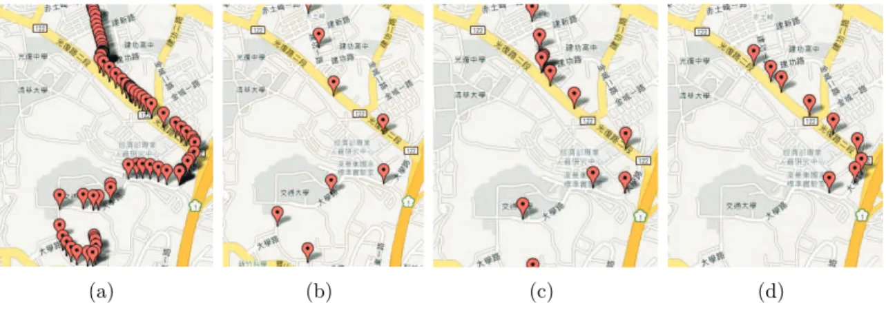
1.1 Some illustrative examples extracted from Carweb datasets. . . 2

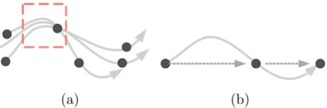
1.2 Two illustrative examples. . . ..3

3.1 Two illustrative examples for _, . . . 12

3.2 Two illustrative examples for observations. . . .13

3.3 An illustrative example of a SC-graph. . . 13

4.1 A scenario of clustering in a dual graph. . . 18

4.2 Distribution of (a) similar and (b) close scores . . . 20

5.1 An illustrative example of our aggregation algorithm . . . 23

6.1 Three experimental results of an existing work. . . 28

6.2 Two experimental results of our approach with (a) Ploss = 0 and (b) Ploss = 0:5. . . 29

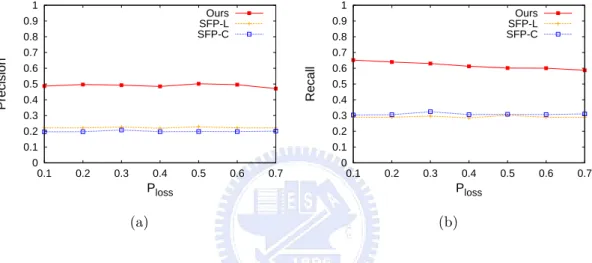
6.3 The impact of Precision and Recall in real datasets with Ploss varied. . . 30

6.4 The impact of Precision and Recall in synthesis data sets with Ploss varied. . . 30

6.5 Similar scores on synthesis datasets. . . 32

6.6 Close scores on synthesis datasets. . . .32

6.7 Successful rate with Ploss varied in (a) real and (b) synthesis datasets. . . .33

6.8 The impact of precision and recall in different

ε

. . . 34

6.9 The values of

λ

and

μ

with

ε

varied. . . 34

6.10 The impact of precision and recall in different

τ

. . . 35

Chapter 1

Introduction

With the pervasiveness of mobile devices, the location of users is easily determined by either GPS devices or some positioning techniques. Furthermore, some softwares are able to log user movements when users go biking and traveling. Thus, a huge amount of movement trajectories are uploaded to some Web community sites [1][2][3]. From such a huge amount of trajectories collected, it is valuable to discover trajectory patterns which represent the moving behaviors hidden in trajectories. Trajectory patterns have been widely utilized in many applications such as trajectory recommendation in some trajectory sharing forums, personalized navigation and data prefetching methods in mobile computing environment.

Given a set of trajectory data, a significant amount of research efforts have proposed approaches of mining trajectory patterns. In general, trajectory patterns indicate sequences of frequent regions that a user usually appears. One of the challenge issues in trajectory pattern mining is how to define frequent region units in trajectory patterns. Previous works for determining frequent regions in trajectory patterns can be generally classified into two categories: the density-based approach and the line-based approach. In the density-based approach, a region is viewed as a frequent region if the number of trajectories passing by is larger than a pre-defined threshold. Furthermore, if nearby regions are also frequent regions, these regions could merge into one larger region. In a line-based approach, a trajectory data is first transformed as a series of line segments. If several line segments from different trajectories are close, a frequent region that contains these line segments is thus determined. The determination of frequent regions is very important since frequent regions are viewed as basic units of trajectory patterns. Without a proper determination of frequent regions, trajectory patterns are not able to capture the moving behaviors hidden in trajectories.

Clearly, the original trajectory data will have an impact on the determination of frequent regions. If the original trajectory data only coarsely capture actual movements of a user,

(a) (b) (c) (d)

Figure 1.1: Some illustrative examples extracted from Carweb datasets.

prior works mentioned above cannot accurately identify frequent regions, let alone deriving trajectory patterns. In reality, there are many factors which affects the capability of original trajectory data capturing the actual movements. To log trajectory raw data, one could set the sampling method and sampling frequency that demonstrate how and how frequent to record the location of a user, respectively. In most positioning device, there are two sampling methods: sampling by distance and sampling by time. In general, setting higher sampling frequency leads to trajectories with more fine resolution. However, setting a higher sampling frequency results in a huge amount of log data generated and the energy exhaustion of logger or GPS-enabled mobile devices. Consequently, a lower sampling frequency is likely to be set and thus trajectory data cannot reflect detailed movements of users. Figure 1.1 shows illustrative examples, where Figure 1.1(a) shows the actual movement, and Figure 1.1(b) and and Figure 1.1(c) are the trajectories following the same movement but sampling by distance and time in a lower sampling frequency, respectively. It can be seen that these trajectories are not accurately capture the actual movement in Figure 1.1(a). In addition, trajectories may be different even if a user who follows the same route. That is, GPS data points in different trajectories that demonstrate the same routing behaviors of that user may not exact the same in terms of locations and times. Figure 1.1(c) and Figure 1.1(d) show two selected trajectories with the same sampling frequency, where a real movement behavior is shown in Figure 1.1(a). Moreover, due to the natural feature of GPS or other wireless network positioning techniques, which refers to the feature that the data point determined has some tolerable errors in terms of the coordinate (i.e., location) and the time, trajectories cannot capture exact the same information of location and time even if the user follows a periodically movement.

From the observations above, prior works of generating frequent regions are not applica-ble since both the density-based and the line-based could not accurately determine frequent regions. For a density-based approach, it is harder to identify frequent regions that contain a

(a) (b)

Figure 1.2: Two illustrative examples.

sufficient amount of data points. For example, the gray lines means the actual movement and the black points are sampled points. Figure 1.2(a) shows that it is possible that the frequent regions (the dashed rectangle) cannot decide accurately by the sampled points. For the line-based approach, the lines derived in a trajectory are likely not to approximate real movement paths and thus, a region that includes more close lines is hardly to derived. For example, in Figure 1.2(b), the actual movement is a S-shape curve but the line segments linked the sampled point are straight. Without a proper design of frequent regions, trajectory pattern mining cannot truly reflect frequent movement behaviors. However, even if trajectories can only reflect partial movements of a user, they reveal some clues about the moving behaviors hidden in trajectories. Consequently, in this paper, we propose an algorithm CACT (standing for Clustering and Aggregating Clues of Trajectories) for discovering trajectory patterns by exploiting such ’clues’. Similar to prior works in [6], trajectory patterns mined in this paper consists of sequences of frequent regions. For each frequent region, there is a representative lines which can capture geometry movements of a user within this region. Exploiting the clues of trajectories, we can distinguish whether trajectories are similar or not. Note that these trajectories may contain a variety of moving behavior of a user. Thus, it’s not appro-priate to put all trajectories together for the determination of frequent regions. Furthermore, to deal with the observations above, we propose a clustering algorithm to divide trajectories into several groups. Trajectories in the same group reflect the same moving behavior of a user and the number of groups is the number of moving behaviors of a user. Then, for each group, we further propose an algorithm to derive a sequence of frequent regions with their corresponding representative line segments. To the best of our knowledge, this is the first work that claims to cluster trajectories into groups first and then derive the corresponding frequent regions within each group. Because of the design, our proposed method of mining trajectory patterns is able to handle the partial information of trajectories (i.e., the clues) and avoid the inaccuracy problem of frequent region determination.

Several challenging issues arise in our proposed method, such as the formulation of simi-larity among trajectories, the clustering algorithm, and the derivation of frequent regions and

representative lines. Since each trajectory some clues for its actual movement, the similarity between two trajectories should be carefully designed. In light of the similarity of trajectories, we could therefore develop a clustering algorithm with the objective of extracting frequent moving behavior of a user. Clearly, the number of groups represents the number of moving behaviors of a user. According to clues of trajectories, each group should include more tra-jectories that are likely to have similar moving behavior so as to fully capture true moving behavior of a user. For each group derived, we propose an aggregation method to aggregate spatio-temporal information of trajectories within the same cluster and generate frequent re-gion sequences. We evaluate our proposed algorithm in both the real dataset and the synthetic dataset. Experimental results demonstrate that our proposed algorithm is able to effectively mine trajectory patterns of a user.

The rest of the paper is organized as follows. Related works are studied in Section 2. Preliminary background is given in Section 2.1. Section 3 describes the proposed similarity for two trajectories. The clustering algorithm for trajectories with the same moving behavior is proposed in Section 4. In Section 5, the aggregation method is then presented. Experimental results are shown in Section 6. Last but not least, we conclude this paper in Section 6.3.

Chapter 2

Related Works

The problem of mining frequent moving patterns has attracted a considerable amount of research efforts. Generally speaking, the flow of mining frequent moving patterns is to first find frequent regions and then derive the relationship between these frequent regions into frequent moving patterns. According to the definition of frequent moving patterns, prior works are generally classified into two categories: spatial movement patterns and spatio-temporal movement patterns. In the first category, a frequent moving pattern refers to a sequence consisting of base station identifications or pre-defined regions. On the other hand, in the second category, frequent moving patterns are able to reflect the spatio-temporal associated relationships among base station identifications or pre-defined regions. For the first category, we mention in passing that the authors in [5] proposed an information-theoretical method to mine frequent moving patterns which are represented as a trie data structure. Moreover, the authors in [23] proposed a statistical approach to mine frequent moving patterns. In [16] and [18], the authors proposed a data mining approach for mining frequent moving patterns with the moving logs of mobile users given.

In the second category, frequent moving patterns are usually extracted from trajectories, where trajectories can reflect the actual movements. A considerable amount of research efforts have elaborated on mining spatio-temporal association rules [17][12][21][22]. In [6], the authors claimed the fuzziness of locations in patterns and developed algorithms to discover spatio-temporal sequential patterns. Furthermore, the authors in [13] proposed a clustering-based approach to discover moving regions within time intervals. In [11], the authors developed a hybrid prediction model, consisting of vector-based and pattern-based model, to predict movements of users. In [9] and [8], the authors exploited temporal annotated sequences in which sequences are associated with time information (i.e., transition times between two movements).

Prior works do not address the issue of geometric inaccuracy of trajectories. To our best knowledge, this is the first work to mine frequent moving patterns from the fragment-information trajectories. The existence of the fragment-fragment-information property brings many challenges since the geometric properties, such as angle, length and direction, cannot be used to find frequent regions directly. Different from the flow of existing works, we find the fragment-information trajectories with potentially the same moving behaviors first, and then use fragment-information trajectories in each cluster to derive a frequent region sequence. As such, our approach can not only tolerate with spatial and temporal but also overcome the geometric inaccuracy of trajectories. These features distinguish our works from others.

2.1

Preliminary

In this section, we present some assumption and notions used in this paper. Then, the problem statement is described. Finally, the overview of our proposed method is given.

2.1.1

Assumptions and Problem Statement

In this paper, we assume that the location of a user is determined by GPS devices or wireless networks. Same as in other works [6][9], a trajectory is defined as follows:

Definition 1. Trajectory representation: A trajectory Ti is a time-ordered sequence

of points, denoted as Ti =< pi,1= (loci,1, ti,1), pi,2 = (loci,2, ti,2), ..., pi,n = (loci,n, ti,n) >, where ti,j < ti,j+1 for all j = 1, 2, ..., n − 1, loci,j is the location at time ti,j and n is the length of Ti.

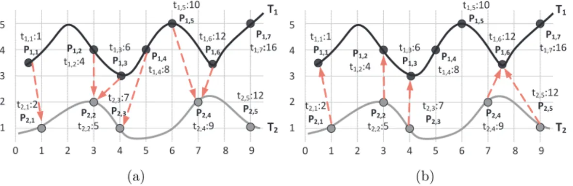
The location determined is represented as the geometry model that consists of the latitude and the longitude of a user. Consider trajectory T1 in Figure 3.1(a) as an example, where the

black curve represents the actual movement and T1 =< p1,1, ..., p1,7 > is a trajectory generated

by GPS devices. As can be seen in Figure 3.1(a), trajectories may not always capture accurate movements of a user. Moreover, according to the setting of GPS logger, a trajectory is in fact represented partial information of a true movement path, which refers to the partial feature of a trajectory in this paper.

Same to prior works [6][9][11], trajectory patterns are sequences of regions, where regions are referred to as hot areas that a user frequently stay or pass by. As pointed out early, a grid-based approach is divided the whole space into grids and the quality of regions is mainly depended on the number of grids. Furthermore, grids may not true capture the movements of a user if the user usually appears in the boundary of grids. Thus, in this paper, we adopt a line-based approach to determine regions for trajectory patterns. Similar to the work in [6],

the region is defined as follows:

Definition 2: Frequent region Given a set of points and a central line L, the region RL

is called a frequent region if the distance between each point p and L is smaller than ² and the number of trajectories that cross over this region is larger than min sup.

In light of the definition of frequent regions, we could therefore give the definition of trajectory patterns mined in this paper.

Definition 3: Trajectory pattern A trajectory pattern considered in this paper is a sequence of frequent regions that contain data points from at least min sup trajectories (referred to relevant trajectories) and each point in relevant trajectories is mapped to one frequent region such that the distance between this data point to the central line of the frequent region is smaller than ².

In this paper, given a set of trajectories, we intend to derive a set of trajectory pat-terns. There are some important observations of trajectories, which provides us some real phenomenon of trajectories, in the real dataset CarWeb[15].

Observation 1: For the same moving behavior, trajectories may have some data bias from the spatial and temporal (i.e., time) perspective. In our collected real trajectories, a user follows the same route to his office. These trajectories are not exact the same in their data points of trajectories. There are some bias in the spatial domain and the time domain. For example, one day, the user is little late to his office and the data points are shifted in the temporal domain. Furthermore, data points in the same location (i.e., one road segment) do not have exact the same location and time information.

Observation 2: Though setting a smaller frequency in our real dataset, the straight line with their two end points as data points in a trajectory is not usually the true movement. This is due to the road networks and the driving speed of a user. For example, if the driving speed of a user is high, the distance between two points in a trajectory is far away and thus the line between these two points cannot accurately approximate the true user movement.

Prior works in [6] that transform the original trajectory into a series of line segments are not applicable to capture the real movements of a user since lines between two consecutive points are not always movement segments of a user. According to the observations above, each data point in a trajectory is viewed as a sampling point of a true user movement. Clearly, if two trajectories have the same sampling frequency to sample the same true movement, each data point from two trajectories is possibly not the same. Since each trajectory is viewed as a sampling from a true movement, with more trajectories for the same true movement, one still could capture true movement of a user. This is due to that data points from different

trajectories that sample the same movement path, still have more possibilities to fall into some spatial areas along with the true movement paths. Furthermore, a user follows several regular true movement paths. For example, a user may have more than one working place and thus he may have more than one regular routings to his working places. Our proposed algorithm can not only mine trajectory patterns with some bias in trajectories data but also discover a set of trajectory patterns that reflect several moving behaviors of a user.

2.1.2

Overview of Our Proposed Algorithm

As mentioned above, trajectories contain partial information of true user movements and data points in trajectories are affected by some bias factors, such as the sampling frequency, positioning delay and time shifts in user movement behavior. Thus, in this paper, we pro-pose an algorithm CACT (standing for Clustering and Aggregating Clues of Trajectories) for discovering trajectory patterns, where clues of trajectories are referred to partial information captured by trajectories. Explicitly, algorithms CACT consists of three phases: In phase 1, we formulate the similarity measurement between trajectories and our similarity formulation will take spatial and temporal bias into consideration. In phase 2, trajectories are clustered into a set of group and trajectories in the same group have similar moving behavior. Furthermore, since trajectories only consider some clues, we should carefully design the clustering method to include trajectories that demonstrate the same moving behavior. In step 3, for each group, we further aggregate trajectories in the same group for deriving a sequence of frequent regions with their corresponding central lines. In the following section, we will describe each step in detail.

Chapter 3

Similarity Measurement

In this section, we derive the similarity measurement for trajectories, which can capture the closeness of trajectories by the clues hidden in trajectories while spatial and temporal bias are taken into account. At first, we define point-to-point similarity to evaluate spatial closeness of two points by considering spatial-bias threshold ². Based on point-to-point similarity, a point-to-trajectory is then defined to find the most near point in a trajectory for the given point by considering the temporal-bias threshold τ . According to the point-to-trajectory, the trajectory-to-trajectory is then defined to evaluate how closeness a trajectory to the other one is by taking both spatial and temporal bias into account. Due to the asymmetric property of the trajectory-to-trajectory similarity, similar and close relations are used to represent that two trajectories behave like each other and just one trajectory behaves like to the other one, respectively. At last, a SC-graph is constructed for representing these two relations among trajectories.

Each trajectory can be viewed as a time series. Therefore, one may use some existing distance measurements for time series to evaluate how similar two trajectories are, such as p-norms, dynamic time wrapping [24][14], and edit-distance-based approaches [4][7]. However, they are hardly applicable these distance measurements to evaluate how similar two trajecto-ries are. Specifically, it is hard to compute distance between two trajectotrajecto-ries by the Euclidean distance (p-norm measurement with p=2), because two trajectories may not have points at the same time unit. Dynamic time wrapping requires each point in a time series to match with the closet point in the other time series such that it cannot tolerate noise and capture the local similar parts between trajectories. Thus, the distance value derived by dynamic time wrapping may significantly increase if the time interval of consequent points in two trajectories are interleaving, or there exists some noises in trajectories. On the other hand, rather than matching all points between two trajectories, the edit-distance-based approach is to match

two time series by allowing some points to be unmatched. Since the length of trajectories with similar moving behavior may vary, the distance value is also affected significantly by the length such that it is hardly used to evaluate how many similar parts between two tra-jectories. Some similarity measurements are designed which also considers the spatial and temporal biases among trajectories [20]. However, they are usually required that there should be points at every time units in each trajectory. If the requirement above cannot be satisfied, interpolation-like approaches may be used to compensate some points for some time units. However, the trajectory may not have points in any time unit. Moreover, compensating points by interpolation cannot reflect the actual movement precisely. The reasons above motivates us to develop a new similarity measurements for trajectories.

To define the similarity for trajectories, we start from the point-to-point similarity: Definition 2. Point-to-Point Similarity: Given a spatial-bias threshold ², and two points pi,` = (loci,`, ti,`) and pj,k = (locj,k, tj,k), the point-to-point similarity is defined as

SP P(pi,`, pj,k) = 1 − dist(pi,`,pj,k)

² where dist(·) is the distance between locations of two points.

To tolerate some spatial bias, a parameter ² is used. The value of point-to-point similarity linearly decays from 1 to 0 by the distance between locations of two points. The closer the two points, the larger the value is. Once the location of two points are exactly the same, the value is 1. On the other hand, once the distance between two points are far from ², the value is 0. For example, consider Figure 3.1(a) and let ² = 10 and Euclidean distance as the distance function, it can be seen that p1,3 is more closer to p2,2 than p2,3 such that SP P(p1,3, p2,2) = 1 −

√ 2

10 = 0.86 > SP P(p1,3, p2,3) = 1 − 102 = 0.8.

Definition 3. Point-to-Trajectory Similarity: Given a point pi,`, a trajectory Tj and

a temporal-bias threshold τ , the point-to-trajectory similarity is defined as SP T(pi,`, Tj) =

max{SP P(pi,`, pj,k)|pj,k ∈ Tj and tj,k ∈ [ti,`− τ, ti,`+ τ ]}.

The idea of point-to-trajectory similarity is to find the nearest point in Tj which time are

allowed within τ time units from pi,`. To facilitate to describe, such a closest point from pi,` is

called the mapped point of pi,`. In practice, there usually exists some temporal bias between

two trajectories even if they follow the same moving behavior. Therefore, τ is introduced to tolerate such temporal bias for fining the mapped point of pi,`. For example, suppose that

we can tolerate the temporal bias to be 3 time units (i.e., τ = 3), to evaluate the point-to-trajectory similarity between p1,2 and T2, three points p2,1, p2,2, and p2,3 are considered since

their time are between t1,2 − 3 to t1,2 + 3 (i.e., 1 to 7). Since SP P(p1,2, p2,2) = 0.8 which

owns the largest value among that from p1,2 to p2,1 and p2,3, the point-to-trajectory similarity SP,T(p1,2, T2) is 0.8.

According to the point-to-trajectory similarity, we can further define the similarity between two trajectories:

Definition 4. Trajectory-to-Trajectory Similarity: Given two trajectories Ti and

Tj, the trajectory-to-trajectory similarity is defined as ST T(Ti, Tj) = P pi,`∈Ti

SP T(pi,`,Tj)

|Ti| .

The trajectory-to-trajectory similarity is used to evaluate how a trajectory Ti is similar

to the other one Tj. The value of ST T(Ti, Tj) is in the interval [0, 1] and determined by the

average of SP T between each point in Ti and its mapped point in Tj with respect to the

length of Ti. Since ST T is derived from SP T and SP P, ST T also takes the spatial and temporal

biases into account. For example, let ² = 10 and τ = 3. In Figure 3.1(a), the arrows show the mapping from each point in T1 to its mapped point in T2. Therefore, we can obtain that ST T(T1, T2) = {SP T(p1,1, p2,1)+SP T(p1,2, p2,2)+SP T(p1,3, p2,2)+SP T(p1,4, p2,3)+SP T(p1,5, p2,4)+ SP T(p1,6, p2,4)}/7 = 0.64.

There are many existing distance or similarity measurement for two time series. However, there are several important properties of ST T, which makes ST T more suitable to measure the

similarity between two trajectories. First, ST T allows the partial mapping for a trajectory to

the other one. That is, a point in a trajectory does not necessary map to a point in the other trajectory. Exploiting such a feature can guarantee each point able to find its mapped point under the spatial-bias and temporal-bias constraint. For example, in Figure 3.1(a), p1,7 has

no mapped point in T2 since there is no points which time is in [16 − 3, 16 + 3]. Moreover,

the location of points in two trajectories may vary even if their moving behaviors are the same. Figure 3.2(b) shows an illustrative example of this case. Through this feature, ST T

can identify only the parts which parts of moving behaviors are likely the same between two trajectories but ignore that are not the same. Second, ST T is noise tolerant. This is a crucial

feature because the location data of a trajectory is inherently inaccurate. With the property of allowing the partial mapping, the value of ST T does not affect significantly by noises because

the noise point will has less probability to be mapped. Third, ST T is asymmetric. That is,

ST T(Ti, Tj) may not equal to ST T(Tj, Ti). For example, Figure 3.1(b) shows the mapping from

T2to T1 and we can obtain that ST T(T2, T1) = 0.77 which does not equal to ST T(T1, T2) = 0.64.

The asymmetry is a very crucial feature since we can use it to distinguish whether a trajectory should be compensated by others or compensate others. The detail will be described later.

From the observation of the asymmetry of ST T, we can define similar and close relations

for any two trajectories.

Definition 5. Similar: Given a threshold λ, a trajectory Ti is similar to the other Tj,

(a) (b)

Figure 3.1: Two illustrative examples for ST,T.

of Ti and T j, SS(i, j), is referred to the value of min(ST T(Ti, Tj), ST T(Tj, Ti)).

Definition 6. Close: Given a threshold µ, a trajectory Ti is close to a trajectory Tj,

denoted as Ti → Tj, if and only if ST T(Ti, Tj) ≥ µ. In brief, the close score from Ti to T j, CS(i, j), is referred to the value of ST T(Ti, Tj).

Conceptually, the similar relation represents that Ti and Tj intend to behave like each

other. That is, they have enough amount of points which are spatially and temporally nearby to each other so that even the minimum value of ST T between them is larger than a given

threshold. Moreover, the similar relation is symmetric such that Ti ∼ Tj implies Tj ∼ Ti.

On the other hand, the close relation only requires that one trajectory behaves like the other one. Thus, the similar relation is not symmetric such that Ti → Tj does not necessarily imply Tj → Ti. Generally speaking, we assume that two similar trajectories implies that they have

close relations between them. In order to achieve the goal, we set a larger value for λ than

µ. Formally, when λ ≥ µ, we can get that Ti → Tj and Tj → Ti if Ti ∼ Tj. As such, in the

following discussion, the value of λ is set to be greater than the value of µ.

Through discovering relations between two trajectories, we are able to distinguish whether a trajectory should compensate its information to others or be compensated by others based on the following observations:

Observations 1 If Ti ∼ Tj, Ti and Tj tend to have the similar length and each point tends

to be able to find its mapped point.

Observation 2: If Ti → Tj, Ti tends to be shorter than Tj and only partial points of Tj

will be mapped from points of Ti.

Figure 3.2 shows two illustrative example for these two observations. In this example, T1

and T3 follow the same movement in the black curve. Similarly, T2 and T4 follow the same

movement in the gray curve. Let ² = 10, τ = 3, λ = 0.9 and µ = 0.85. In Figure 3.2(a), it can be derived that ST T(T2, T4) = 0.92 and ST T(T4, T2) = 0.92. Thus, T2 ∼ T4. It can

(a) (b)

Figure 3.2: Two illustrative examples for observations.

Figure 3.3: An illustrative example of a SC-graph.

be observed that the length of T2 and T4 are likely the same and only p2,2 is not mapped

when computing ST T(T4, T2). Based on this observation, we can conclude that a set of the

trajectories which are mutually similar represent potentially the same moving behavior. On the other hand, Figure 3.2(b) shows the opposite case from the former one. In the similar fashion, we can obtain that ST T(T1, T3) = 0.52 and ST T(T3, T1) = 0.93. Therefore, T3 → T1.

It can be seen that T3 is shorter than T1 and only three points in T1 are mapped. In this

case, it can be observed that through adding three points in T3, T1 can be compensated and

describe the moving behavior between p1,1 to p1,2 more precisely. Overall, the close relation

is helpful for identifying which trajectories can compensate others.

The similar and close relations can describe the different functionalities when mining tra-jectory patterns. Exploiting such relations, we can identify whether a tratra-jectory should be compensated by others or compensate others. Therefore, a SC-graph is constructed to repre-sent the both relations among trajectories:

Definition 7. SC-Graph: Given a set of trajectories T = {T1, T2, ..., Tn}, a SC-graph

weight wS(vi, vj) = min(ST T(Ti, Tj), ST T(Tj, Ti)) if Ti ∼ Tj, and (vi, vj) ∈ EC with its weight

wC(vi, vj) = ST T(Ti, Tj) if Ti → Tj and Ti  Tj.

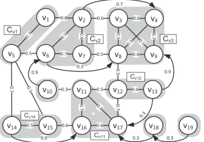
In a SC-graph, each vertex represents a trajectory. Once two trajectories are similar to each other, an undirected edge is then constructed between them. On the other hand, a directed edge will be constructed if one trajectory is close to the other one. Since two similar trajectories are required to be close to each other, a directed edge only exists when a trajectory is close to the other but they are not similar to each other. For example, let λ = 0.5 and

µ = 0.3, Figure 3.3 shows an illustrative example of a SC-graph. To facilitate to describe, a

vertex in a SC-graph is equivalent to a trajectory, an edge in ES is called a similar edge, and

Chapter 4

Clustering Trajectories

Since the given trajectories may contain more than one moving behavior, it is required to distinguish the trajectories with the same moving behaviors and group them into clusters. In this section, we describe our approach for grouping trajectories with similar moving behavior into clusters.

In Section 3, we introduce a SC-graph to present similar and close relations between trajec-tories. As such, the similar and close edges in a SC-graph represent some clues that indicates whether two trajectories represent the similar moving behavior or not. Thus, clustering tra-jectories with the similar moving behavior can be viewed as the procedure of exploiting some clues to clustering vertices in a SC-graph. To realize this idea, some definitions are elaborated in the following.

Definition 9. Core: Given a SC-graph G = (V, ES ∪ EC) and a threshold δ, a vertex u ∈ V is a core if there exists a set of vertices Cu such that 1. for v ∈ Cu and v 6= u,

(u, v) ∈ ES, and 2. for all v, w ∈ Cu, (v, w) ∈ ES, and 3. |Cu| ≥ δ.

A core u in a SC-graph is a vertex with sufficient trajectories similar to it and these trajectories are mutually similar. Thus, a core set Cu contains trajectories which can most

likely represent the same moving behavior. The value of δ is usually set to be at least 2 since the moving behavior described by a trajectory which is not similar to anyone is not enough confident. For example, let δ = 2, v2 is a core and Cv2 = {v2, v6, v7} where v6 and v7 are the

neighboring vertices of v2 in ES, each vertex has similar edge to others, and |Cv2| = 3 ≥ δ = 2.

Even if some trajectorie follows the same moving behavior, it is possible that they are not in the same core due to the natural of trajectories. However, some ’clues’ may exist to indicates two cores with the similar moving behavior. This definition is elaborated in the following.

vertex v, denoting as u à v, if v is a core and u is adjacent to v in ES or EC.

Directly clue-reachability shows a vertex u with the same moving behavior to a core. A vertex u can show it following the same moving behavior of a core through a similar or a close edge, respectively. Obviously, all vertices in Cv are mutually directly clue-reachable.

For example, v5 Ã v6 since v6 is a core and (v5, v6) ∈ ES; v1 Ã v2 since v2 is a core and

(v1, v2) ∈ EC.

Through the directly clue-reachability, we can find those vertices which potentially repre-sent the similar moving behavior as a core. In the following definition, we extent the directly clue-reachability to clue-reachability which can describe a vertex following the similar moving behavior through many clues indirectly.

Definition 11. Clue-Reachable: A vertex u is clue-reachable to a vertex v, denoting as u Ã∗ _{v, if there exists a chain of vertices v = v}

1, v2, ..., vn = u such that vi à vi+1 for all i = 1, 2, ..., n − 1.

For example, v5 Ã∗ v8 through the path v5 Ã v6 Ã v7 Ã v8.

Based on clue-reachability, we can further define the clue-connection from one core to the other core as follows:

Definition 12. Clue-Connect: A core u is clue-connected to v if there exists a core w such that x Ã∗ _{y for all x ∈ Cu and for some y ∈ C}

w, and y 0

Ã∗ _{z for all y}0

∈ Cw and for

some z ∈ Cv.

Conceptually, through clue-connection, we can imply the moving behavior of a core u is similar to that of a core v. To ensure sufficient clues to support that, each vertex in Cu should

be clue-reachable to some vertices of an intermediate core sets. That is, all vertices in Cu,

i.e., trajectories stating the similar moving behavior of u, should follow the similar moving behavior as an intermediate core set. Similarly, all vertices in this intermediate core sets should follows the same moving behavior as the core v. For example, v11 is clue-connected to v8. It can be seen that there is a core v5 such that all vertices in Cv11 are clue-reachable to

some vertices in Cv5 (i.e., v11 Ã v5 and v10 Ã v5), and all vertices in Cv5 are clue-reachable

to some vertices in Cv8 (i.e., v1 Ã

∗ _v

3 and v5 Ã∗ v8).

For a core, there may be several cores clue-connected to it. To ensure that trajectories with the most similar moving behavior are grouped into a cluster, we derive a measurement

clue-gain to evaluate how much ’clue’ a core set can obtain via the other one.

Definition 13. Clue-Gain: Consider two sets S and T . Let Est

S and ECst be the set of

similar and close edges from S to T , respectively. The clue-gain ClueGain(S, T ) = α × |Est

S| × P e∈Est wS(e) + β × |Est C| × P e∈Est wC(e).

Generally speaking, more similar/close edges from S to T implies that S is more likely to represent the similar moving behavior as T . Also, the weights between these edges should be taken into account. The higher weights of these edges, the more similar the moving behaviors of S and T . Therefore, the clue-gain is proportional to the number of similar and close edges and the corresponding weights from S to T . Moreover, the similar edges should be weighted higher than the close edges because the similar edges represent that the moving behaviors of two vertices are mutually similar and the close edges only represents the moving behavior of one vertex is like to the other. Thus, two constants α and β are used for weighting the similar and close edges, respectively. Usually, the value of α should be at least two times larger than

β. By the definition of similar and close scores, SS(i, j) = min(ST T(Ti, Tj), ST T(Tj, Ti)) ≤ ST T(Ti, Tj) = CS(i, j). Thus, 2SS(i, j) ≤ CS(i, j) + CS(j, i), which shows that one similar

edge is at least two times important as a close edge. Thus, α should be set two times larger than β.

For example, let α = 2 and β = 1. ClueGain(Cv12, Cv3) = 2 × 1 × 0.5 + 1 × 1 × 0.9 = 2.9

and ClueGain(Cv12, Cv11) = 2 × 2 × (0.5 + 0.7) + 1 × 1 × 0.3 = 5.1. Obviously, Cv12 intends to

show more similar moving behavior to Cv11 than Cv3 since there are more similar edges from

Cv12 to Cv11 than to Cv3.

According to the clue-connected and the clue-gain, we can formulate the problem of clus-tering trajectories with similar moving behavior as follows:

Definition 14. Cluster: A cluster C is a set of vertices satisfying the following conditions: 1. for all u ∈ C, there exists a core v ∈ C such that u is clue-connected to v (connectivity); 2. for all core sets Cu ∈ C, the core set Cv which can induce ClueGain(Cu, Cv) maximal is

also in C (compactness); 3. |C| ≥ min sup (frequentness).

The first requirement states that a cluster is composed of many cores which have clues to support them describing the similar moving behavior. The second requirement describes the compactness of a cluster, where each core set should be in the same cluster with the core set which can make the clue-gain maximal. That is, each core set is used to interpret the moving behavior with the strongest clues from this core set. On the other words, a core set will not interpret the moving behavior with weaker clues. To ensure derived regions being frequent, a cluster should contain more than min sup vertices which is describing in the third statement. We propose a clustering algorithm to find clusters in a SC-graph. In nut shell, this algo-rithm first discovers all core sets, then merges them according to their clue-gains, and adds some non-cores into clusters for enriching information of clusters at last. The algorithmic form is listed in Algorithm 1.

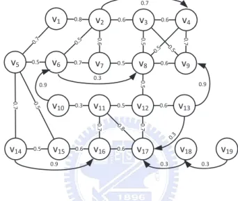
Figure 4.1: A scenario of clustering in a dual graph.

Note that a core set in a SC-graph is equivalent to a clique with size ≥ δ on ES. Thus,

in the beginning, we find a clique cover on ES, where a clique cover refers to a set of clique

with their union being the whole graph. There are many existing heuristic algorithm to find a clique cover efficiently [10]. One of famous heuristic algorithms is based on greedy strategy which idea is to always select the highest degree vertex, and to pick its adjacent vertices which have edges mutually to form a clique. For example, v8 owns the highest degree in this graph

(only considering ES). There are five vertices adjacent to it, say v7, v3, v4, v9, and v13. It

can be verified that only v3, v4, and v9 have edges between each other. Thus, the first clique {v3, v4, v8, v9} is then generated. Cliques of a clique cover in our example are shaded in Figure

4.1.

After finding a clique cover, we can identify those clique with size ≥ δ as the core sets. For example, let δ = 2, Cv1, Cv2, Cv3, Cv11, Cv12, and Cv14 are core sets. As long as

deriv-ing the core sets, each core set computes the clue-gain from it to all one-step clue-connected core sets. Then, a core set is merged to the core set with the maximal clue-gain. For ex-ample, for Cv12, there are two one-step clue-connected core sets Cv3 and Cv11 with the

clue-gains ClueGain(Cv12, Cv3) = 1.9 and ClueGain(Cv12, Cv11) = 5.1, respectively. Thus, Cv12

is merged with Cv3 rather Cv11. The other example is that Cv14 is merged with Cv1 due to

ClueGain(Cv14, Cv1) = 4.8 > ClueGain(Cv14, Cv11) = 2.1. Similarly, Cv1 is merged into Cv2

and Cv2 is merged into Cv3. Consequently, we can derive two clusters: {Cv1, Cv2, Cv3, Cv14}

and {Cv11, Cv11}. It is worth mentioning that the merged cliques are guaranteed to be

clue-connected since each clique can be only merged with its one-step clue-clue-connected clique, thereby satisfying the requirement 1 and 2 of a cluster. At last, some cliques with size ≤ δ are con-sidered to join some clusters to compensate the moving behaviors represented by this cluster. As such, a non-core joins a cluster with a core which can induce the maximal clue gain. In

this case, a non-core does not merge the other non-core because a chain of non-cores with dif-ferent moving behavior may be contained in a cluster, especially for non-cores with only one vertex. For example, v18 and v19 form such a chain. It can be seen that the v18 is close to v17

which indicates it can compensate the information of Cv11. However, it is not obvious whether

v19 can be used to compensate or not. After that, clusters with less than min sup vertices

and the remaining non-cores are eliminated. Following the example, let min sup = 5. The cluster {Cv11, Cv11} and the vertex v19 are eliminated. Consequently, there are two clusters

{Cv1, Cv2, Cv3, Cv14, v10} and {Cv11, Cv12, v18} as the final results.

Algorithm 1: Clustering Trajectories Input : A SC-graph: G = (V, ES∪ EC) Output : A set of clusters: C

C ← φ;

1

K = {K1, K2, ..., Km} ← a clique cover of G; 2

CORE ← cliques in K with the size ≥ δ;

3

for each clique Ki in CORE do 4

Compute the clue-gain with all one-step clue-connected cliques in CORE; 5

Ci= Ki; 6

add Ci into C; 7

for each clique Ki in CORE do 8

Kmax← the clique in CORE which can maximize ClueGain(Ki, Kmax); 9

Cmax← the cluster containing Kmax; 10

Cjoin← the cluster containing Ki; 11

Cmax← Cmax∪ Cjoin; 12

for each clique Kj in K − CORE do 13

Kmax← the clique in some Cmax which can maximize ClueGain(Kj, Kmax); 14

Put Kj into Cmax; 15

Selection of Thresholds

The selection of thresholds usually depends on user’s requirements and the properties of the environment. However, setting λ and µ are not straightforward tasks. The selection of thresholds highly affects the structure of a SC-graph since the number of edges significantly depend on the thresholds for similar and close relations (i.e., λ and µ). The larger λ and µ restrict whether two trajectories have similar and close relations or not more seriously. Thus, larger thresholds incur the fewer edges in a dual graph and make a dual graph more sparse. A cluster in a sparse dual graph may contain only few trajectories such that it is hard to aggregate them to obtain the frequent movement precisely. The smaller λ and µ makes a dual graph more dense. However, it is easy for a cluster to contain more irrelevant trajectories such that the frequent regions cannot be derived precisely. Therefore, the results of clustering are highly dependent on the values of λ and µ.

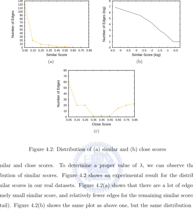
0 10 20 30 40 50 60 70 80 90 100 110 120 130 0.05 0.15 0.25 0.35 0.45 0.55 0.65 0.75 0.85 Number of Edges Similar Score (a) 0 1 2 3 4 5 6 7 8 -4.5 -4 -3.5 -3 -2.5 -2 -1.5 -1 -0.5

Number of Edges (log)

Similar Score (log) (b) 0 10 20 30 40 50 60 70 80 0.05 0.15 0.25 0.35 0.45 0.55 0.65 0.75 0.85 Number of Edges Close Score (c)

Figure 4.2: Distribution of (a) similar and (b) close scores

of similar and close scores. To determine a proper value of λ, we can observe that the distribution of similar scores. Figure 4.2 shows an experimental result for the distribution of similar scores in our real datasets. Figure 4.2(a) shows that there are a lot of edges with extremely small similar score, and relatively fewer edges for the remaining similar scores (i.e., long tail). Figure 4.2(b) shows the same plot as above one, but the same distribution shows itself to be linear on a log-log scale, which is the characteristic signature of the power law distribution. Thus, by the observations above, we can conclude that the similar scores follow the power law distribution.

As such, the threshold λ should not be these small similar score since it will make a dual graph too dense. In this case, we should not select the threshold λ to be 0.05. To prevent the threshold λ too large, a heuristic approach to select the threshold λ is to select the average similar score in the long tail. For the efficiency sake, the long tail can be simply determined by 80-20 principle where we suppose that the edges with 20% largest similar score form the long tail [19]. In our example, the edges with similar score larger than 0.15 form the long tail. On the other hand, Figure 4.2(c) shows that the distribution of the close scores tends to have two peaks. Note that the close relation is used to identify which trajectories should provide information to compensate the other one. Therefore, to prevent less trajectories with different moving behavior to put into a cluster, the edges with lower close score should not exist in

a dual graph. As such, the threshold µ can be selected to be the average of all close scores which value can keep the right peak and discard the left peak. In this example, the value of

µ is set to be about 0.4. In our latter experimental results, we will show that the heuristic

Chapter 5

Aggregation Phase

In clustering phase, the trajectories are divided into several clusters where each cluster con-tains more than min sup trajectories. In this phase, the spatial and temporal information of trajectories in a cluster will be aggregated and then a frequent region sequences is generated for each cluster.

The trajectories in a cluster may represent the same moving behavior. However, it is not a trivial task to aggregate the information of these trajectories because there may exist some spatial bias, temporal bias, and noise data in them. To overcome these issues, a trajectory which can best represent the moving behavior of trajectories in a cluster will be chosen. Such a trajectory is referred as to the kernel. The information of other trajectories are adjusted to compensate the kernel. Once obtaining the compensated kernel, the coming issue is how to decide the minimal number of regions which can satisfy the spatial bias threshold ².

Since the weight of two similar edges represents how much these two trajectories are similar to each other, the vertex which the highest total weights of the similar edges incident to refers the trajectory which the most trajectories in a cluster are similar to. For example, in Figure 4.1, v3 is the kernel in the cluster {Cv1, Cv2, Cv3, Cv14, v10}. Note that the kernel is likely from

more larger cores. A larger core has more mutually similar vertices such that each vertex has more similar edges incident to it. The total weights of a vertex in a larger core is more easily larger than that in a smaller core. In addition, we have more confident to the moving behavior describing by a larger core than a smaller one. It satisfies that we shall select the trajectory which can most represent the moving behavior of this cluster. Moreover, a larger core tends to have more close edges incident to it. It also follows the intuition that the kernel can be compensated the moving behavior from other trajectories.

Since not all information of trajectories can be used to compensate the kernel, the order of adding trajectories should be carefully decided to make as more trajectories able to compensate

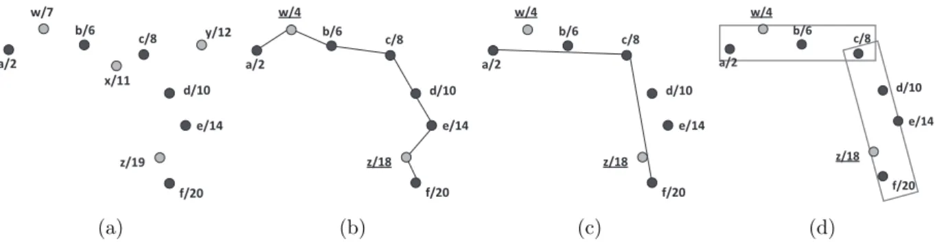
(a) (b) (c) (d) Figure 5.1: An illustrative example of our aggregation algorithm

their information to the kernel as possible. As such, the trajectories which are most likely similar to the kernel should be first considered. To evaluate how a trajectory is similar to the kernel, we should first consider the minimal steps from the trajectory to the kernel, which can be done by BFS. Once a vertex can achieve the kernel by fewer edges, this vertex has less spatial and temporal bias to the kernel with higher probability. Moreover, the path that induces the minimal steps from the trajectory to the kernel is also important. Product of the weights along the path implies that how much this trajectory is similar to the kernel transitively. Overall, the trajectory with smaller BFS steps and the higher product of weight along its BFS path should be first considered. For example, consider the cluster {Cv1, Cv2, Cv3, Cv14, v10} in

Figure 4.1. In this cluster, the kernel is v3. The vertices v6 and v7 are two-step far from the

kernel. From v6 to v3, the maximal product of weight is 0.5 × 0.6 = 0.3. From v7 to v3, the

maximal product of weight is 0.5 × 0.5 = 0.25. Thus, v6 has higher priority to compensate

the kernel than v7 does.

After deciding the order of compensating the kernel, the next task is to adjust the spatial and temporal information of other trajectories such that these information can be used to compensate the kernel. The concept of our aggregation algorithm can be best understood by the example in Figure 5.1. Suppose that the black points are from the kernel and the grey points are from the compensating trajectory. The number associated with each point represents the time. In the beginning, all points of the compensating trajectory are spatially projected as shown in Figure 5.1(a). Among the compensating points, The point w has some temporal bias with the kernel because it locates between kernel points a and b but the value of time of w is not between that of a and b. The point x has such temporal bias as well. In addition, the point y is a noise point which is too far from the other points. Then, according to the points of the kernel, the temporal information of compensating points will be adjusted. Suppose that a compensating point p locates between two kernel points q and r. If p is between [tq− τ, tr+ τ ] where τ is the temporal-bias threshold, then its time is adjusted by the

the point is discarded. Such adjustment is reasonable because a temporal-bias τ is allowed when computing the similarity between two trajectories. For example, let τ = 2. Suppose that the distance between a and w equals to that between b and w. Since the time of w is 7 which is between [2 − 2, 6 + 2], the time of w is adjusted as 2 + (6 − 2) × _{dist(a,w)+dist(w,b)}dist(a,w) = 4. On the other hand, the time of x is 11 which is outside the interval [6 − 2, 8 + 2]. Thus, the compensating point x is discarded. In the similar fashion, the time of z is adjusted to 18. Next, the noise points are discarded. Following the notations above, the point p is a noise point if dist(p, qr) > ². The point y is the noise point and thus eliminated. Figure 5.1(b) shows the results after adjusting the temporal information and eliminating noise points. The procedure repeats until all compensating trajectories are added.

Algorithm 2: Aggregation Algorithm Input : A set of clusters: C

Output : A set of frequent region sequences: R for each cluster K ∈ C do

1

Tker← the kernel trajectory of C; 2

for each vertex v ∈ K do Compute its BFS steps and largest weight product to the kernel; 3

for each trajectories T in the descending order of BFS steps and weight products do 4

Spatial projection all points of T ; 5

for each points p do 6

q, r ← two points in the kernel that p locates between them;

7

if tp ∈ [tq− τ, tr+ τ ] and dist(p, qr) ≤ ² then 8 tp= tq+ (tr− tq) ×_{dist(p,q)+dist(p,r)}dist(p,q) 9 else 10 discard p; 11 end 12 end 13

L ← lines obtaining by Douglas-Peucker algorithm;

14

Ω ← regions by central lines L; 15

Add Ω into R; 16

end 17

After adding all compensating points, Douglas-Peucker algorithm are used to determine the number of regions. The purpose of this algorithm is that finding the minimal line segments which the distance of each point to the corresponding line is smaller than a threshold ². Therefore, the minimal number of regions can be obtained while the distance between each point to the line can be guaranteed to be smaller than a threshold ². Conceptually, the algorithm recursively divides the line. Initially a line segment with the first and the last points is constructed. If the farthest point to the line segment is closer than ², it represents the point can be represented by this line. Otherwise, if the point furthest from the line segment is greater than ², the original line segment will be separated into two line segments at this point. The algorithm recursively calls itself until the distance of all points to the derived lines are smaller than ². Taking the line segments in Figure 5.1(b) as input, Figure 5.1(c) shows the

final results where two line segments are derived. Consequently, by viewing the derived lines as the central lines, the regions can be easily derived. The final results are shown in Figure 5.1(d).

Chapter 6

Performance Evaluation

In this section, the effectiveness and efficiency of mining trajectory patterns from trajectories are evaluated. In Section 6.1, we present the environments and settings in our experiments. All experiments are conducted by both the synthesis dataset and the real dataset. The comparison between our approach and the existing work are shown in Section 6.2. Sensitivity analysis in several parameters are also investigated in Section 6.2.1.

6.1

Experimental Environment

In our experiments, both real and synthesis datasets are used to evaluate the existing works and the proposed methods. For real datasets, we extract trajectories from a GPS-based testbed, CarWeb, which aims at collecting real trajectories of users [15]. In CarWeb system, each user can obtain his location from GPS every five seconds and upload his location to the

CarWeb server. Note that, we can manually category the trajectories in CarWeb dataset such

that we could have the ground truth about the moving behaviors represented by trajectories. In our experiments, we choose three kinds of trajectories which represents 3 kinds of frequent moving behaviors and one kind of trajectories which represents infrequent ones. Specifically, there are 30, 20, and 10 trajectories with 300, 130, and 500 points in average, respectively. There are 3 infrequent trajectories with 160 points in average. On the other hand, for synthetic datasets, we construct a simulator to generate many synthetic trajectories by given source trajectories as inputs. The source trajectories we extract are generated in a very high sampling rate and we also manually adjust them to ensure the correctness. Each synthetic trajectory is a variant from a input trajectory, where the time of each point may shift by t time units and the location of each point may shift by the angle θ and the distance r in a probability pbias.

for spatial bias), respectively. In our simulation, there are four kinds of source trajectories, which have 3000, 4000, 5000, and 6000 points, respectively. To simulate the different sampled rates, we induce the loss rate Ploss to determine the probability of a point in a highly-sampled

trajectory will be discarded. Explicitly, each point in a trajectory is discarded with probability

Ploss. Thus, a trajectory tends to be more inaccurate from the real movement under a higher

loss rate. The default value of parameters are listed as follows: τ = 30 minutes, ² = 10 meters, min sup = 0.1, the total number of trajectories is 200, r = 5 meters, t = 30 minutes,

Pbias = 80%, and Ploss= 50%.

For the comparison purposes, the method of mining spatio-temporal frequent patterns in [6], denoted by SFP, is implemented. Since this approach is not designed for mining trajectory patterns from trajectories, we exploit linear interpolation and cubic spline interpolation to estimate the locations for low-sampled trajectories and use these compensated trajectories as inputs of SFP, say SFP-L and SFP-C. Also, since SFP cannot cluster trajectories with the different moving behavior, the inputs of SFP are the trajectories with the same moving behaviors.

To evaluate experimental results, three performance metrics, precision, recall and execution

time, are used. Since both SFP and our methods use a sequence of spatial regions to represent

the frequent patterns from trajectories, a smaller region may cover less road segments, which can describe which road segments are frequent more precisely. Since the both datasets are obtained from the movement on a road network, each data point in a trajectory can be also bind with a road segment id. Thus, a trajectory can represent as a sequence of road segments. By presenting each trajectory into a sequence of road segments, the conventional approaches for mining frequent itemsets, such as apriori, can be used to find frequent road segments from the given trajectories. The precision is used to evaluate how precise the derived frequent regions in different approaches. Let C be the road segments covered by the derived regions and F be the frequent road segments. The precision is formulated as

L(C ∩F )/(L(C ∩F )+L(C ∩ ¯F )), where L(·) represents the total length of the roads. A higher

precision value means that the derived region tends to cover more frequent road segments and fewer infrequent ones. On the other hand, the recall is used to evaluate the area that the derived regions can cover the frequent road segments derived by apriori. The recall is formulated as L(C ∩ F )/(L(C ∩ F ) + L( ¯C ∩ F )). A higher recall value means that more

frequent road segments can be covered by the derived region. At last, the execution time is used to measure the efficiency and the scalability of the proposed method.

(a) (b) (c)

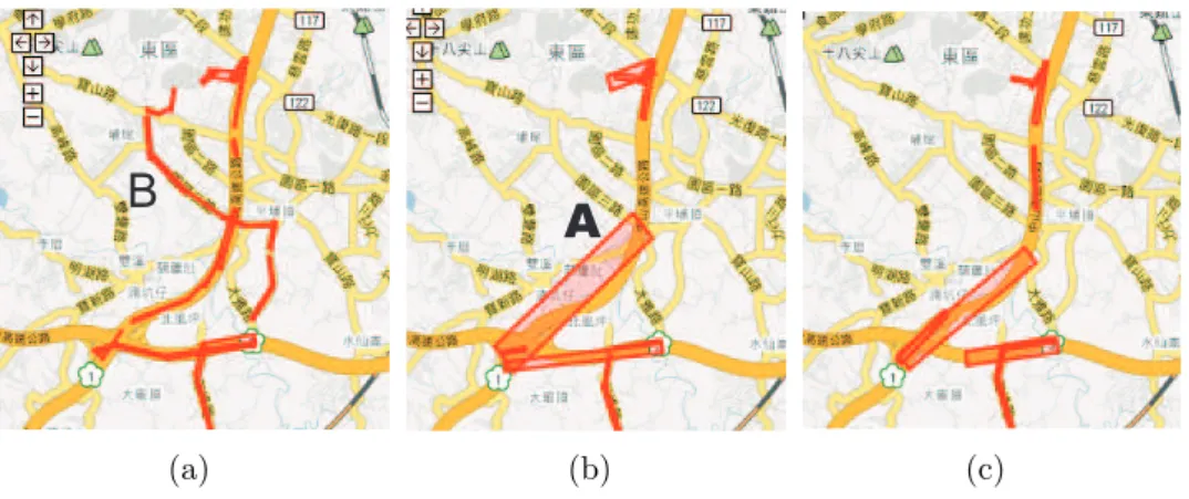
Figure 6.1: Three experimental results of an existing work.

6.2

Comparison with SFP

In this section, we evaluate our approach and SFP in terms of the visualized results, the precision and the recall.

We first show the frequent regions discovered from real datasets in a visualized manner. Figure 6.1(a) shows the result of SFP when the given trajectories are manually compensated and corrected the position of each point. The derived regions are thin and located on the road segments, which are consistent with the fact that trajectories in a road network moves on roads. Then, consider lossrate = 50%, the derived regions derived by SFP is shown in Figure

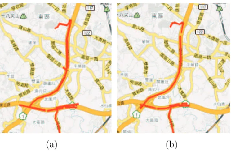
6.1(b). It can be seen that region A locate outside the road segments, which are inconsistent to the fact of the movement on a road network. Moreover, some regions disappear. To deal with the problem, one may propose that interpolation can be used to compensate the location data between the remaining points. Given the compensated trajectories, Figure 6.1(c) shows the derived regions. Comparing with Figure 6.1(b), such strategy is effective because more derived regions locate on the roads, especially the two regions at the center. However, it still does not work well because some frequent regions are still missing. In brief, from these experimental results, we can observe that the frequent regions cannot be derived precisely, even incorrectly, by the line-based approach.

As mentioned above, there are four kinds of moving behaviors within the given trajectories in real datasets. Figure 6.2 shows one of the frequent regions which is found by our approach. Comparing the results of SFP in Figure 6.1(a) and that of our approach in Figure 6.2(a), it can be seen that the frequent regions found by two approaches are similar, which shows our approach can also find frequent spatio-temporal regions found by SFP. Moreover, the common regions in Figure 6.2(a) and Figure 6.1 represent the most frequent road segments among trajectories. Figure 6.2(b) shows the result with Ploss = 0.5, which the derived regions