嫌惡設施與不良環境對於房價影響之估計---大量估價法與分量迴歸模型之比較

行政院國家科學委員會專題研究計畫 成果報告

嫌惡設施與不良環境對於房價影響之估計：大量估價法與

分量迴歸模型之比較(第 2 年)

研究成果報告(完整版)

計 畫 類 別 ： 個別型

計 畫 編 號 ： NSC 96-2415-H-004-011-MY2

執 行 期 間 ： 97 年 08 月 01 日至 98 年 07 月 31 日

執 行 單 位 ： 國立政治大學經濟學系

計 畫 主 持 人 ： 林祖嘉

計畫參與人員： 碩士級-專任助理人員：陳湘菱

報 告 附 件 ： 出席國際會議研究心得報告及發表論文

處 理 方 式 ： 本計畫可公開查詢

中 華 民 國 99 年 01 月 05 日

風水對於商用不動產價格影響之估計：

大量估價法與分量迴歸估計法之比較

*

林祖嘉，政大經濟系特聘教授

馬毓駿，政大經濟系博士生

2009.12

摘要

風水一直是國人擇居與進行商業活動的考量因素之一，本研究根據現有的文

獻與實際的觀察發現，對高價位的商用住宅而言，不論是擁有者或租賃者對規避

嫌惡性設施的願付金額對低房價的商用建物都來得較高，反映在建物價格上，對

建物價格的抵減亦必然高於低價位者。本計畫遂嘗試以分量迴歸模型來驗證此一

立論，實證結果發現，屬於較高價位的商用建物對嫌惡性設施的反應明顯高於低

價位者，其效果甚至達 2 倍以上的幅度，此一證據顯示，規模較大的公司企業對

於顯惡性設施的厭惡程度遠高於規模較小者。

關鍵字：分量迴歸模型、嫌惡性設施、房價

JEL Classification：R31

*作者感謝國科會研究計畫(NSC-96-2415-H-004-011-MY2)之財務協助。本文為初

稿，未經作者同意，請勿引用。

1.前言

風水一直以來是影響華人住宅興建、搬遷或購屋時的一個重要考量，以經濟

學的語言而言，多數人主觀上認定好風水所能產生的邊際效用甚高，因而願意支

付的邊際成本甚至高於其餘建物特徵。以 Bourassa and Peng (1999)研究華人

世界裡風水對於房價的影響，且認為華人深信風水一說，認為好的風水將為民眾

帶來好的運氣，反之則會帶來壞的時運。林秋綿(2007)研究，發現購屋者在選購

房屋時會考慮嫌惡風水的影響程度，且他們對嫌惡風水所採取的措施有，不購

買、要求降價求售和請風水師解決等。Tam et al.(1999)以 1996 年香港大埔東

一帶之十五個村落共 3400 戶人家的普查資料，探討房價與風水的關係，其結果

發現風水、交通可及性和房齡，以風水和屋齡較為顯著。而對於造成此一現的原

因，來自於多數人建物本身所在位置、周圍環境能與大自然的磁場結合，進而對

居住或從事商業活動的人能夠產生無形的助力，當擁有好的周圍環境時，即好的

風水，信此道者相信此一無形助力將更為明顯，對於居住人的健康或或公司事業

將更能提供助益。反之，不好的風水則會致使住所或辦公所在地無法與大自然的

磁場產生連結，進而當事人於居住或從事商業活動時，可能產生心神不寧或進行

錯誤決策的機率增加。

雖風水的影響在主觀上普遍對多數國人購屋、裝修等相關活動有顯著的影響，但

是否因此而轉嫁到建物價格上，以及其影響程度的大小則仍有賴有效的估計加以

判定。理論上，如將風水如同鄰里環境一般視為建物特徵之一，如嫌惡性設施，

不好的風水環境會使建物價格下降，好的風水環境則會使得建物價格上升。

Bourassa and Peng 的研究即指出，由於華人家庭將門牌號碼視為風水的一環，

因此門牌號碼都會影響房屋價格，當非華人購屋者認為未來在房屋轉售時買主有

可能會是華人，他們有誘因選購有幸運門牌號碼的房屋，所以這些住宅的價格相

對較高。而除傳統觀點將特殊地形視為風水要件之一外，許多現代性設施亦被視

為風水要件之一，如火葬場、公墓、殯儀館、屠宰場、垃圾掩埋場、煤氣供應站、

監獄和機場都是高度的嫌惡設施等，即使對當地居民進行某些實質補貼，但會遭

受當地居民的抗爭。李永展、何紀芳(1996) 以問卷調查台北地區的居民對於嫌

惡設施的看法，發現火葬場、公墓、殯儀館、屠宰場、垃圾掩埋場、煤氣供應站、

監獄和機場都是高度的嫌惡設施，平均有 80%的民眾反對該公共設施於住家附

近。Smith and Desvousges(1986)的研究亦有類似結論，居住地與廢棄物基地距

離會影響房屋價值。而這些嫌惡性設施對房價的負面影響亦如如不好的風水一

般，許多國內外的研究都已證實嫌惡性設施對房屋價格有不利的影響。

雖不好的風水或嫌惡性設施對房價有抵減的效果，但實際上，因購屋人特

徵、房屋用途或房屋本身的價值對壞風水及嫌惡性設施的反應都不相同。白金安

(2002) 以高屏地區的居民為問卷施測對象，發現隨宗教信仰、教育程度、和房

屋類型的不同，對於風水的見解有所差異，進而使風水對房價影響程度也隨之不

同。舉例來說，家庭所得越高或家庭資產淨值越高，則通常對於嫌惡性設施的厭

惡程度會比所得及資產淨值較低者來得高，或者說厭惡程度相同但因財富差距因

而願規避嫌惡性設施的願付金額不同，而通常家庭淨資產或所得月高者通常願意

支付的金額來的更大，反之，家庭收入及財富較低者，願付的規避金額就來得較

低。而購屋需求與住宅品質的要求，一般而言與家庭收入及淨資產有高度相關，

所得及財富越高者，通常住宅需求的品質越高，亦隱含房價越高，因此嫌惡性設

施產生的邊際負效用在資本化後，對高房價的影響必然高於低房價建物。

除嫌惡性設施對住宅用途房價的影響可能因房價高低而有所差異，對於商業

用途房價的影響可能是相同的情況，舉例來說，高總價的商業用途房屋的擁有者

或承租公司，同常會是具有高邊際收益的公司或資本額在一定程度以上的企業，

對於各種可能影響獲利的情況都會考量在其中，而風水因素於心理層面或實質面

或多或少都對企業主於建廠、營業單位設置或挑選具有一定的影響性，且往往願

意支付極高的價格來規避不好的風險。當資本額或營業額越大的公司，主觀上對

於嫌惡性設施或風水不佳的厭惡程度會相較資本額或營業額較小者來得高。在吾

人假設資本額或營業額較大的企業，能夠購買或承租的商業用建物價格皆較高，

反之，則較低。在此條件下，本文推論嫌惡性設施或壞風水對於價格較高的商業

用途建物影響，必然高於價格較低者。

為驗證此一立論，本文採用分量迴歸(Quantile Regression)模型來解釋顯

惡性設施對不同價位商業用住宅價格的影響，理論上，由於分量迴歸將被解釋變

數依研究者設定劃分為數個分量，每個分量都包含完整的解釋變數，當被解釋變

數及解釋變數的關係因不同分量而有所差異時，便可透過分量迴歸模型掌握此一

現象。以本計畫而言，如將嫌惡性設施及壞風水視為建物特徵之一，如吾人先前

所推論，價格越高的商業用建物代表規模較大的企業，且願意支付的規避金額亦

較高，則當建物周圍存在這些不好環境時，對於房價的影響必然高於低房價者。

實證結果指出，當商業用途建物的價格越高時，嫌惡性設施對房屋價格的減損程

度逐漸提高，且在對高分量(90%以上)的影響幾乎為較低者(10%以下)的兩倍。

最後，本計畫架構如下：第一節說明本計畫的研究動機，第二節分量迴歸模

型介紹，第三節說明本研究的資料來源、基本性質，第四節說明估計結果，第五

節為結論。

2.分量迴歸模型

以下對於分量迴歸模型的推導，主要參考 Kuan(2007)分量迴歸講義和葉憶

婷(2007)。設 Y 是一隨機變數，其分配為

F 和

Y

θ

_，

θ

∈(0,1)。

F 的

Y

θ

_分量為

( )

q Y

_θ

_{，我們取反函數則可得}

F q

_Y

( )

=

θ

_，如：

{

}

1 ( ) Y ( ) inf ; y( ) q Yθ =F−

θ

= y F y ≥

θ

₍₁₎

則 Y 當中就有小於和大於

q Y

θ

( )

_{的比例，就會呈現}

θ

_比(1-

θ

_{)，然後我們給予這}

些離差絕對值(1-

θ

)和

θ

的權重，運用與最小平方法相同的求解方式，求得

q Y

θ

( )

| | ( ) (1 ) | | ( ) ( ) ( ) (1 ) ( ) ( ) Y Y y q y q Y Y y q y q y q dF y y q dF y y q dF y y q dF y

θ

θ

θ

θ

> < > < − + − − = − − − −

∫

∫

∫

∫

然後再對上式取一階微分，可得

0

_Y

( ) (1

)

_Y

( )

y q

dF y

y q

dF y

θ

θ

> <

= −

∫

+ −

∫

( ) Fy q

θ

= − +

換句話說，即

( )

arg min[

|

|

_Y

( ) (1

)

|

|

_Y

( )]

y q y q

q Y

_θ

θ

y

q dF y

θ

y

q dF y

> <

=

∫

−

+ −

∫

−

同理若在兩個隨機變數之下，給定 X 之下，Y 的條件累積機率分配為

FY X|

_，所以

( )

q X

_θ

_為

| | ( ) ( )

( )

arg min[

|

|

_{Y X}

( ) (1

)

|

|

_{Y X}

( )]

y q x y q x q

q X

_θ

θ

y

q dF

y

θ

y

q dF

y

> <

=

_∫

−

+ −

_∫

−

(2)

若

x 和

i

y ，

i i=1, 2,...,n

_{是從隨機變數 X 和 Y 所抽取的 n 個樣本觀察值，則 Y 的}

條件分量

q X

θ

( )

_{可由下式估計}

( ) ( ) 1 ( ) arg min | ( ) | (1 ) | ( ) | i i i i i i i i i q y q x y q x q X y q x y q x N θ

θ

θ

≥ ≤ ⎡ ⎤ = _⎢ − + − − _⎥ ⎣

∑

∑

⎦

且假設

x 和

i

y 為線性模型，

i i i i

y

=

x

′

β

+

e

_;

其中被解釋變數

yi

為

1 1×

的向量，解釋變數

x 為 1

i

k

× 的向量，係數 β 為 1

k

× 的向

量，誤差

e 為

i 1 1×

_{的向量。則 y 的第}

θ

_{樣本之條件分量為}

q X

θ

(

i

)

=

x

i

′

β

_。根據(2)

式，y 的第

θ

樣本條件迴歸係數

β

θ

_{可以表示為下式的解}

1 arg min | | (1 ) | | i i i i i i i i y x y x y x y x N θ _β β β

β

θ

β

θ

β

′ ′ ≥ ≤ ⎡ ⎤ ′ ′ = _⎢ − + − − _⎥ ⎣

∑

∑

⎦

₍₃₎

令

sgn(

y

_i

−

x

_i

′

β

)

=

1,

,

1,

.

i i i i

if y

x

if y

x

β

β

′

>

′

−

<

則第(3)式可以改寫為下式，

1 1 1 1 arg min [ sgn( )]( ) 2 2 N i i i i i y x y x N θ _β

β

θ

β

β

= ′ ′ =

∑

− + − −

(4)

然後對第(4)式取一階微分，得到

1 1 1 1 0 [( sgn( )) ] 2 2 N i i i i y x x N =

θ

β

′ =

∑

− + −

(5)

若第(4)中

y

i

=

x

i

′

β

，則不可微分，在估計分量迴歸係數時，將產生困難。

β

θ

在

描述當解釋變數

x 變動一單位時，被解釋變數

i

y 的第

i

θ

分量將變動

β

θ

單位。

三、分量迴歸之大樣本性質

令

1

1

( ,

, )

sgn(

)

2

2

i i i i i

x y

β

θ

y

x

′

β

x

Φ

= − +

−

對 ( , , )

Φ

x y

i i

β

取期望值，則為

1

1

[ ( ,

, )]

[

sgn(

) ]

2

2

i i i i i

x y

β

E

θ

y

x

′

β

x

Ε Φ

=

− +

−

| | |

1

1

[

sgn(

)

|

]

2

2

1

1

[ (

(sgn(

) |

))]

2

2

1

1

[ (

(1

1

|

))]

2

2

1

1

[ (

(1

(

)

(

))]

2

2

[ (

(

))]

i i i i i i i i i i i i i y x y x i i y x i y x i i y x i

y

x

x x

x

y

x

x

x

x

x

F

x

F

x

x

F

x

β β

θ

β

θ

β

θ

θ

β

β

θ

β

′ ′ > <

⎧

_′

⎫

= Ε Ε − +

_⎨

−

_⎬

⎭

⎩

′

= Ε

− + Ε

−

= Ε

− + Ε

−

′

′

= Ε

− +

−

−

′

= Ε

−

(6)

其中

Ε(1y_i<x_i′β|xi)=Fy x| (xi′

β

)

_、

Ε(1y_i>x′_iβ |xi)= −1 Fy x| (xi′

β

)

_，且1

A

為 A 的 indicator

function。

給定

x 之下，

i

| (yi xi′

β

θ |xi) FY X(xi′

β

)

θ

Ρ < = =

，

表示在

θ

分量之下，

y 小於

i

x

i

′

β

θ

的機率等於

θ

。因此當

β β

=

θ

時，

| [ ( ,x yi i, )]

β

[ (xi

θ

Fy x(xi′

β

))] 0 Ε Φ = Ε − =

上式用來估計

β

θ

_{的條件動差為 GMM 特例，所以我們可以套用 GMM 的估計方法的}

大樣本理論，得到

1 1 ( ) (0, ) A N

β

_θ −

β

_θ ∼ N Τ Π Τ_θ− _{θ θ}−

₍₇₎

其中

( , , ) [ ( , , ) ( , , ) ] i i i i i i x y x y x y θ θ θ

β

β

β

β

∂ΕΦ Τ = ∂ ′ Π = Ε Φ Φ

在

β β

=

θ

[ ( ,

x y

_{i i}

, ) ( ,

x y

_{i i}

, ) ]

θ

β

β

′

Π = Ε Φ

Φ

1 1 {[ [ (1 1 | )]] 2 2 1 1 [ [ (1 1 | )]] } 2 2 1 1 {[ [ ( (1 | ) (1 | ))]] 2 2 1 1 [ [ ( (1 | ) (1 | ))]] } 2 2 1 1 {[ [ (1 (1 | 2 2 i i i i i i i i i i i i i i i i i i i y x y x i i y x y x i i y x i y x i i y x i y x i i y x i x x x x x x x x x x x x β β β β β β β β β

θ

θ

θ

θ

θ

′ ′ > < ′ ′ > < ′ ′ > < ′ ′ > < ′ < = Ε − + Ε − ′ − + Ε − = Ε − + Ε − Ε ′ − + Ε − Ε = Ε − + − Ε 2 ) (1 | )]] 1 1 [ [ (1 (1 | ) (1 | )]] } 2 2 {[ [ (1 | )]][ [ (1 | )]] } { ( 1 ) } i i i i i i i i i i i i y x i i y x i y x i i y x i i y x i i y x i x x x x x x x x x E x β β β β β β

θ

θ

θ

θ

′ < ′ ′ < < ′ ′ < < ′ < − Ε ′ − + − Ε − Ε ′ = Ε − Ε − Ε ′ = Ε −

且

| |

( ,

,

)

[ (

(

))]

[

(

)]

i i i y x i i i y x i

x y

x

F

x

x x f

x

θ θ θ θ θ θ

β

β

θ

β

β

β

∂ΕΦ

Τ =

∂

′

∂Ε

−

=

∂

′

_′

= −Ε

其中又因為

e

( )

θ

= −

y x

′

β

_θ

，所以

( )|

[

x x f

_{i i e x}

(0)]

θ

′

θ

Τ = −Ε

若給定

x 下，

i 1yi<x′iβθ

服從 Bernoulli 分配，其期望值為

θ

，變異數為

θ

(1−

θ

)

，

所以

Π

θ

_{可改寫為，}

(1 ) (x x_{i i} ) θ

θ

θ

′ Π = − Ε

在實務上

Τθ

_{較容易被估計，但是由於}

Π

θ

_{依條件分配}

fe( )|θ x

_{而不同，因此難以估計。}

當

fe( )|θ x(0)= fe( )θ (0)

_{，也就是誤差項的機率密度函數在 0 時和 x 是彼此獨立的，}

則可以簡化

Ω

，其中

1 1 ( )| ( )| 1 2 ( )

( ,

,

) ( ,

,

)

[

(0)]

(1

) (

) [

(0)]

(1

) (

)

(0)

i i i i i i e x i i i i e x i i e

x y

x y

x x f

x x

x x f

x x

f

θ θ θ θ θ

β

β

θ

θ

θ

θ

− − −

′

Ω = Φ

Φ

′

′

′

= Ε

− Ε

Ε

′

− Ε

=

則也可以將第(7)式化為

1 2 ( ) (1 ) ( ) ( ) (0, ) (0) A i i e x x N N f θ θ θ

θ

θ

β

−

β

∼ − Ε ′ −

(8)

但由於其中誤差項的條件機率密度難以估計，所以我們利用統計軟體 STATA 內的

拔靴法(bootstrapping)，以自體重複抽樣的方法，估計變異數矩陣。

1

3. 資料來源及基本統計量

1

本計畫的資料來源為國內某一家商業銀行承做的商業用途房屋貸款資料，樣

本數共計有 10669 筆，除房屋價格之外，建物特徵計有面積、是否擁有車位、總

樓層高度、所在樓層、屋齡、臨路路寬、公設比、所在樓層是否為一樓及本計畫

關注的嫌惡性設施。

2

對於嫌惡性設施對建物價格的影響，本計畫採用累計的方

式表示對房價的影響，在所有樣本中，緊鄰 1 項嫌惡性設施的有 957 個觀察值，

緊鄰 2 項及 3 項嫌惡性設施的樣本則分別有 41 個及 4 個觀察值。對於本計畫採

用的其他連續性變數，本文一律以對數化處理，並加入二次式效果檢驗對建物價

格是否存在非線性的影響，其餘變數如是否擁有車位、所在樓層是否為一樓其

23 縣市(台北市為標準組)為虛擬變數，公設比原始值即為比例，本計畫於估計

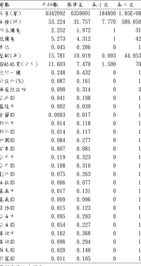
時維持原數值亦不測試其二次式的非線性效果。研究基本統計量如表 1 所示。

4. 實證結果

於執行分量迴歸之前，吾人先以 Belsley et al.(1980)發展的 DFFITS 指標

剔除樣本離群值，其公式如下：

) ( ) (

)

(

ˆ

ˆ

i i i

h

s

i

y

y

DFFITS

=

−

其中

yˆ 為第 i 個觀察值的預期值，來自於迴歸模型使用所有樣本點進行估計，

_i

)

(

ˆ i

y

為第 i 個觀察值的預測值，但估計迴歸式為未包含第 i 個樣本點下的模型所

進行的預測值，

s 為不包含第 i 個樣本值下的估計標準差，

_(i)

h 定義為 hat matrix

_(i)

即

x

_i

(

X

′

X

)

−1

x

_i

′

， p 為模型中的參數估計值、

n

為總樣本數，當

DFFITS

>

2

p

n

便

刪除此一樣本。本文為例，原始觀察值為 10664 筆，最小平方法中的參數估計值

p 為 35 個，經計算後共計剔除 605 個離群值。

2

嫌惡性設施項目詳見附件。

表 1 基本統計量表

變數

平均數

標準差

最小值

最大值

房價(萬)

6342092

6359091

184800 1.95E+08

面積(坪)

53.224

31.757

7.770

589.050

所在樓層

2.252

1.972

1

31

總樓層

5.273

4.312

1

42

車位

0.045

0.206

0

1

屋齡(年)

15.781

10.019

0.003

44.953

臨路路寬(公尺)

11.603

7.470

1.500

70

位於一樓

0.248

0.432

0

1

公設比(%)

0.087

0.161

0

1

嫌惡性設施

0.099

0.314

0

3

台北縣

0.041

0.198

0

1

基隆市

0.002

0.039

0

1

宜蘭縣

0.0003

0.017

0

1

新竹市

0.014

0.118

0

1

新竹縣

0.014

0.117

0

1

桃園縣

0.084

0.277

0

1

苗栗縣

0.007

0.081

0

1

台中市

0.119

0.323

0

1

台中縣

0.108

0.310

0

1

彰化縣

0.075

0.263

0

1

南投縣

0.006

0.077

0

1

嘉義市

0.017

0.131

0

1

嘉義縣

0.009

0.096

0

1

雲林縣

0.015

0.123

0

1

台南市

0.095

0.293

0

1

台南縣

0.054

0.227

0

1

高雄市

0.162

0.368

0

1

高雄縣

0.096

0.294

0

1

屏東縣

0.020

0.140

0

1

花蓮縣

0.011

0.105

0

1

資料來源：本研究。

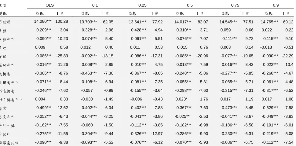
於執行分量迴歸估計時，為方便描述建物特徵與嫌惡性設施在不同價格分量

下的影響，本計畫以每 0.05 分量做一次分量迴歸，共計執行 19 次分量迴歸式，

並表列相關文獻常用的五個條件分量(0.1,0.25.0.5,0.75,0.9)的估計結果進行

實證說明，並比較與最小平方法下估計結果的差異，其結果如表 2 所示。同時吾

人進一步將 19 個分量下各參數估計係數值繪於圖中，以便觀察每一建物特徵在

不同分量下對建物價格的影響變化，圖中水平的實線為最小平方法估計所得的餐

數值，上下兩條水平需線為其 95%的信賴區間；分量迴歸所得到的結果為實心的

曲線，上下兩條需線的曲線為其 95%的信賴區間，如圖 1 所示。

表 2 分量迴歸估計結果

模型 OLS 0.1 0.25 0.5 0.75 0.9 變數 係數 T 值 係數 T 值 係數 T 值 係數 T 值 係數 T 值 係數 T 值 截距項 14.080*** 100.28 13.703*** 62.05 13.641*** 77.92 14.017*** 82.07 14.545*** 77.51 14.765*** 69.12 面積 0.209*** 3.04 0.328*** 2.98 0.428*** 4.94 0.310*** 3.71 0.059 0.66 0.022 0.22 面積平方 0.090*** 10.23 0.074*** 5.40 0.061*** 5.51 0.076*** 7.07 0.111*** 9.72 0.115*** 9.10 車位 0.009 0.58 0.012 0.40 0.011 0.53 0.015 0.76 0.003 0.14 -0.013 -0.51 屋齡 -0.086*** -25.83 -0.092*** -13.15 -0.086*** -17.31 -0.085*** -20.96 -0.077*** -19.65 -0.090*** -22.29 屋齡平方 0.016*** 11.26 0.008*** 2.85 0.010*** 4.75 0.013*** 7.59 0.016*** 8.43 0.022*** 10.4 總樓層 -0.306*** -8.76 -0.463*** -7.30 -0.367*** -8.05 -0.248*** -5.86 -0.277*** -5.85 -0.260*** -4.67 總樓層平方 0.071*** 8.44 0.108*** 6.94 0.081*** 7.35 0.055*** 5.31 0.065*** 5.71 0.061*** 4.48 所在樓層 -0.246*** -7.62 -0.057 -0.99 -0.155*** -3.64 -0.298*** -7.60 -0.315*** -7.31 -0.317*** -6.52 所在樓層平方 0.004 0.33 -0.030 -1.49 -0.006 -0.43 0.023* 1.76 0.017 1.19 0.017 1.08 路寬 0.499*** 12.62 0.402*** 6.04 0.402*** 7.88 0.367*** 7.63 0.473*** 8.45 0.529*** 7.98 路寬平方 -0.052*** -6.43 -0.044*** -3.25 -0.041*** -3.86 -0.025** -2.53 -0.041*** -3.67 -0.049*** -3.83 位於一樓 -0.162*** -7.55 -0.060 -1.50 -0.112*** -3.85 -0.182*** -6.98 -0.186*** -6.58 -0.191*** -6.01 公設比 -0.275*** -11.55 -0.304*** -9.44 -0.326*** -12.97 -0.286*** -9.90 -0.230*** -6.31 -0.219*** -5.08 鄰嫌惡設施 -0.090*** -9.38 -0.093*** -5.52 -0.076*** -6.12 -0.070*** -5.93 -0.086*** -6.75 -0.112*** -7.54 資料來源：本研究整理。 附 註：為節省篇幅，區域虛擬變數估計值不逐一表列。

面積 -0.4 -0.3 -0.2 -0.1 0 0.1 0.2 0.3 0.4 0.5 0.6 0.7 0.05 0.15 0.25 0.3 5 0.45 0.55 0.6 5 0.75 0.8 5 0.95 面積平方 0 0.02 0.04 0.06 0.08 0.1 0.12 0.14 0.16 0.18 0.05 0.15 0.25 0.35 0.45 0.55 0.65 0.75 0.85 0.95 車位 -0.15 -0.1 -0.05 0 0.05 0.1 0.15 0.05 0.1 0.15 0.2 0.25 0.3 0.35 0.4 0.45 0.5 0.55 0.6 0.65 0.7 0.75 0.8 0.85 0.9 0.95 屋齡 -0.12 -0.1 -0.08 -0.06 -0.04 -0.02 0 0.05 0.15 0.25 0.35 0.45 0.55 0.65 0.75 0.85 0.95 屋齡平方 0 0.005 0.01 0.015 0.02 0.025 0.03 0.035 0.05 0.15 0.25 0.35 0.45 0.55 0.65 0.75 0.85 0.95 總樓層 -0.7 -0.6 -0.5 -0.4 -0.3 -0.2 -0.1 0 0.05 0.15 0.25 0.35 0.45 0.55 0.65 0.75 0.85 0.95

估計結果顯示，面積及其二次式效果對建物價格有正面的影響，其中二次式

效果隨著建物價格越高，其邊際影響性越大。車位因素未顯示對商用建物價格有

顯著的影響，此一結果與分析住宅用途建物價格有較大的差異。代表折舊的屋齡

在不同分量亦顯示對建物價格有抵減效果，而其二次式效果進一步指出，此一折

舊效果隨著屋齡愈大，其折舊的速度越快，同時不同分量下的參數估計值進一步

顯示，此一加速折舊現象在高價位的商用住宅更為明顯。

總樓層平方 0 0.02 0.04 0.06 0.08 0.1 0.12 0.14 0.16 0.05 0.15 0.25 0.35 0.45 0.55 0.65 0.75 0.85 0.95 所在樓層 -0.6 -0.5 -0.4 -0.3 -0.2 -0.1 0 0.1 0.05 0.15 0.25 0.35 0.45 0.55 0.65 0.75 0.85 0.95 所在樓層平方 -0.08 -0.06 -0.04 -0.02 0 0.02 0.04 0.06 0.08 0.1 0.05 0.15 0.25 0.35 0.45 0.55 0.65 0.75 0.85 0.95 路寬 0 0.1 0.2 0.3 0.4 0.5 0.6 0.7 0.8 0.9 0.05 0.15 0.25 0.35 0.45 0.55 0.65 0.75 0.85 0.95 路寬平方 -0.12 -0.1 -0.08 -0.06 -0.04 -0.02 0 0.05 0.15 0.25 0.35 0.45 0.55 0.65 0.75 0.85 0.95 1樓 -0.35 -0.3 -0.25 -0.2 -0.15 -0.1 -0.05 0 0.05 0.05 0.15 0.25 0.35 0.45 0.55 0.65 0.75 0.85 0.95 公設比 -0.4 -0.35 -0.3 -0.25 -0.2 -0.15 -0.1 -0.05 0 0.05 0.15 0.25 0.35 0.45 0.55 0.65 0.75 0.85 0.95 嫌惡設施 -0.2 -0.18 -0.16 -0.14 -0.12 -0.1 -0.08 -0.06 -0.04 -0.02 0 0.05 0.1 0.15 0.2 0.25 0.3 0.35 0.4 0.45 0.5 0.55 0.6 0.65 0.7 0.75 0.8 0.85 0.9 0.95

圖 1 建物特徵分量迴歸趨勢圖

而總樓層高度對建物價格的影響為負，同時其二次式效果為正，此一估計結

果與住宅用途建物的分析略有不同，在住宅為用途之下，總樓層高度通常反映其

建築成本，因而對建物價格的影響通常為正。對商用住宅而言，建築成本於構成

商業用途建物價格中的地位可能不如住宅用途來得大，因而總樓層高度可能有其

他未量化的經濟含意，而未能反映於資料型態中，此一部分仍有待本計畫未來更

進一步的探討。在所在樓層方面，其反應出入的便利性的效果相當顯著，當樓層

越高價格越低，且隨著建物價格越高，此一效果更行顯著。

路寬的影響亦符合吾人的預期，大體而言，臨路的路寬越寬時價格越高，此

一估計結果仍是反應對外的便利性，亦符合林祖嘉和洪得洋(1999)研究結果，道

路寬對對於房屋價格有正向的影響，且對於商用型態的房屋其影響程度相較於其

他住宅型態更大。而當建物位於 1 樓時，則顯示對建物價格有不利的影響，此一

結果應與從事的商業活動有關，唯資料無法進一步獲得相關訊息，仍需留待後續

研究進行探討。公設比則普遍對建物價格有不利的影響，因其表示可用的私人空

間受限之故。本計畫關注的嫌惡性設施方面，其估計結果顯示在每個分量對建物

價格都產生相當顯著的抵減效果，而此一效果隨著建物價格越高其邊際效用越

強，符合吾人事前推論高總價商用建築的企業主通常更為重視嫌惡性設施及風水

的影響。

5. 結論

相信風水對居住人或從事商業活動有不好影響一直以來是華人世界的認

知，在寧可信其有的情況下，反應至居住或進行商業活動的建物將可能產生價格

抵減的作用。本文以商用住宅為例說明風水與嫌惡性設施對建物價格的衝擊，同

時吾人推測當建物價格較高時，代表企業主對於風水的關注程度更高或願付更高

的金額來規避其影響，故嫌惡性設施與壞風水對高價位商用建築的影響必然高於

低價位建物。本計畫採用分量迴歸模型來驗證此一假設，其實證結果符合吾人所

預期，當建物價格越高時，嫌惡性設施及壞風水對建物價格的影響越高，以較高

價位的 10 的分量而言，其影響幾乎為低價位建物的兩倍。

參考文獻

白金安、李春長、潘淑惠、紀心怡、張小倚、湯茹茵(2002)，“家庭型態差異對

購屋行為之影響-以高雄市為例”，2002 年不動產經營系暨休閒事業經營系學

生畢業專題報告發表會論文

，

國立屏東商業技術學院。

李永展、何紀芳，1999，“環境正義與鄰避設施選址之探討”，規

劃學報

，26，

第 91-107 頁。

林秋綿(2007)，“風水因素對不動產價格影響之探討”，

土地問題研究季刊

，6(1)，

第 45-52 頁。

林祖嘉、洪得洋(1999)，“臺北市捷運系統與道路寬度對房屋價格影響之研

究”，

住宅學報

，8，第 47-67 頁。

Bourassa, S. C., and V.S. Peng (1999), “Hedonic Prices and House Numbers:

The Influence of Feng Shui,” International Real Estate Review, 2(1), 79 – 93.

Kuan, C. M. (2007), An Introduction to Quantile Regression, Institute of

Economics Academia Sinica.

Belsley, D. A., E. Kuh, and R. E. Welsch (1980), Regression Diagnostics,

New York: John Wiley & Sons.

Tam C. M., Y. N. Tso, and K. C. Lam (1999), “ Feng Shui and Its Impacts on Land

and Property Development,” Journal of Urban Planning and Development, 125(4),

pp.152-163.

Smith, V. K., and W. H. Desvousges (1986), “The Value of Avoiding a Lulu:

Hazardous Waste Disposal Sites,” The Review of Economics and Statistics, 68(2),

pp.293-299.

附錄一

附表一：嫌惡設施一覽表

項目

項目

近殯儀館

路沖

近墳場

近加油(氣)站

近火葬場

廢氣污染區

近高壓電塔

鐵道旁

近變電所

噪音污染區

近爆竹廠

近神壇或廟

近瓦斯儲存槽

近特種行業

近瓦斯廠

高架道旁

近棺木店

基地低於路面

近地下油行

近安養院

資料來源：本研究。

出席國際學術會議心得報告

計畫編號 NSC 96-2415-H-004-011-MY2 計畫名稱 嫌惡設施與不良環境對於房價影響之估計：大量估價法與分量迴歸模型之比較（第 2 年） 出國人員姓名 服務機關及職稱 林祖嘉 政大經濟學系 教授 會議時間地點 Los Angels

會議名稱 2009AsRES & AREUEA International Conference

發表論文題目 Tenure Choice, Demand for Mortgage, and Saving Behavior: An Evidence from

Taiwan.

2009AsRES 及 AREUEA 聯合年會會議心得報告

政大經濟系教授 林祖嘉 2009.7.15 2009 年亞洲不動產學會(AsRES) 與美國不動產與都市經濟學會(AREUEA)聯合 年會，在 2009 年 7 月 11 日到 14 日在美國洛杉磯加州大學(UCLA)安德森管理學院 舉行。全部共有 181 篇文章發表，全部參與的教授人數約達到 250 人以上。台灣大 約有超過 30 位教授參與，共有 25 篇文章發表。 AsRES 與 AREUEA 每年一次的聯 合年會可能是在不動產領域中，規模最大的年會之一，也是最重要的年會之一。 今年的大會上邀請的 keynote speaker 是 UCLA 管理學院的教授 Richard Roll， 講題是”The Possible Misdiagnosis of a Crisis. ” 其內容主要在探討我們對於去年全球 金融海嘯可能的錯誤解讀。另外，在一場午餐會中，美國住宅與都市部(Housing and Urban Department, HUD) 的副部長說明金融海嘯之後，美國應付金融海嘯的主要住 宅政策為何。同時，他也指出金融海嘯之後美國住宅政策的重要性大增；而且政府 部門對於住宅相關研究的重視程度也大幅提升，這對於我們學者而言可以說是一個 還算不錯的消息。

本人這次發表的文章是”Tenure Choice, Demand for Mortgage, and Saving

Behavior: An Evidence from Taiwan. ” 我們先利用 nested logit model 來估計台灣人民 對於租買的選擇，以及是否貸款的選擇。然後再利用 Heckman selection model，來 估計人們在考慮租買選擇與貸款選擇之後，人們的儲蓄行為如何受到影響。 由於這是國際學術界上在討家計單位的儲蓄行為時，很少計論到的層面，因此 本文在會議上受到相當多的注意，而且會場上提問的人也很多。我們一方面很高興 文章受到重視；另一方面，我們也得到很多的建議與評論，這不但對於未來我們在 修改本文時會有很大的助益，而且對於未來文章能在國際學術期刊上發表的機會也 提高許多。所以，我們參加這次會議的收獲可以說是相當的大，參加會議的目的也 可以說是圓滿的達成。

1

附件

Tenure Choice, Demand for Mortgage, and Saving Behavior:

An Evidence from Taiwan

Chu-Chia Lin*

Department of Economics National Chengchi University

Chien-Liang Chen**

Department of Economics National Chi Nan University

Keywords: saving, tenure choice, mortgage

JEL classification: D12, D63, R21

This paper is prepared for the Joint 2009 AsRES-AREUEA International Conference, July 11-14, 2009, Los Angelse, California, USA.

*Correspondence author. 64, Sec. 2, Chi-Nan Rd., Taipei 116, Taiwan. Tel: 886-2-29387462; E-mail:

[email protected].

2

Abstract

This study use Survey of the Family Income and Expenditure (SFIE) to investigate the interactions between household characteristics, demographic structures and housing tenure choice. Employing multi-nominal logit and nested logit models, we are able to clarify the mechanisms of tenure choices determined through household income and demographic factors. In addition, we estimate the saving functions of various types of households with the consideration of sample selections. It is suggested that homeowners without mortgage save the most than others. Furthermore, household size and income are positively correlated with saving.

3

1.

Introduction

Housing plays a dual role in view of housing demand of the household. On the one hand, housing provides services for residence such as the consumption side, on the other hand, housing could be an investment. According to the calculation of Lin and Lin (1994), two thirds of the housing demands in the Taiwan area are of the investment purpose, while only one third of the demands belong to the actual housing consumption purpose. Due to the high housing price, home buyers usually have to put into consideration the assets they possess in addition to income level. Although the percentage of the purchasing loan from domestic banks could go as high as 80%, the bank would usually underestimate the value of housing when providing loans. According to the estimation of Lin (1991) and Lin and Lin (1996), domestic housing loan in average takes up approximately only 60% of the actual housing price. Since the financial market is not well developed in Taiwan, it is thus required for the buyers to pay a great amount of down payment when purchase housing.

Under the circumstance, it is clear that housing purchase is a crucial decision for most households. The essential for home buyers is to prepare enough assets to meet the need of down payment. Due to the restrictions on domestic data, it has become one of the major issues for researchers to deal with income level only when estimating housing demands. A great deal of literature has been discussing the relationship among income, housing demand and housing price, e.g., Wu (1994). A lot of literatures have estimated the income elasticity on housing demand; refer to Deng (1985), Jia (1983), Lin (1988) and Lin and Lin (1994) and Wu (1981). With the lack of data on wealth, researchers often overlook the influences that wealth might bring about when calculating housing demand. As income and wealth both have positive influences over housing demand, and that wealth and income are often positively correlation with each other, it is thus understandable that the income elasticity on housing demand would be overestimated were health effects being neglected.

However, when income and housing price are both considered at the same time in Lin and Lin (1994), the estimated income elasticity goes as high as 1.298 for self-owned housing in the Taiwan area. This figure is way above the generally accepted empirical income elasticity estimation, 0.75, of Polinsky (1977) and Polinsky and Ellwood (1979) by using the U.S. data. Lin and Lin (1994) explained the higher income elasticity result as that Taiwanese people purchase housing with part of investment incentive. On the other hand, it might a reflection that the wealth variable is neglected in Lin and Lin (1994) and income effect is thus overestimated. Chen and Lin (1998) estimated the income and wealth effect of Taiwanese housing demand in 1981 and 1990. Their finding of income elasticity of

4

housing demand is very closed to that of Polinsky (1977) and Polinsky and Ellwood (1979). Furthermore, they concluded that, for owners, the level of wealth significantly affects housing demand and the effect increases as the level of wealth increases. For renters, asset elasticity of housing demand is insignificant.

The purpose of this study is to estimate housing demand behavior with respect to various types of household composition, i.e., two generation with income in contrast with only one generation with income in a household. In particular, we would be very keen to understand whether there is difference between the income effects of two individual generations. This issue is related to intra-household resource allocation and has not been fully extrapolated yet. As has mentioned above, housing price is high in Taiwan. Housing purchase is not an easy task for young adult families. Like Japan, young adult children might tend to live with elder parents to reduce housing expenditure. There are a substantial number of extended families in Taiwan, these families provide us the opportunity to estimate housing demand function and compare with that of nuclear families.

As for rental housing, the story might be different. Although wealth effects usually influence people’s demands on housing services, when the family is actually renting a house unit, their only purpose is to consume the housing services, and with no investment purpose attached. Within this research framework, we also estimate demand of rent housing of various types of household composition, considering the income and wealth variables at the same time.

Following this introduction, we first establish a simple housing demand function in section 2. we include the characteristics of a family in addition to income and wealth. Consequently, we describe the data that is used, and the estimated demand function in section 3. In this study, we use the raw data of the Survey of Family Income and

Expenditure (SFIE) from DGBAS, distinguishing self-owned housing and rented housing, so as to estimate the housing tenure choice under different types of household compositions. Section 4 is the conclusion.

2. Housing Demand Function

Assume that individual household i contains household characteristicsxi j _{with tenure}

choices j. The random utility function of household i chooses j is expressed as:

ij i ij j ij

5

Where

ε

ij is residual. At the beginning, we firstly treat the three types of

tenure choice as individual and independent and that can be formulated under a multi-nomial logit model. Assume Equation (1) follow Gumbel distribution, a multi-nomial logit model can be derived fro each household i with choice j:

1

(

,

)

ij j ij j i ij ij x y J x y j

P

P U

U

j

J

e

e

β α β ′ α ′ ′ + + ′=

′

=

>

∀ ∈

=

∑

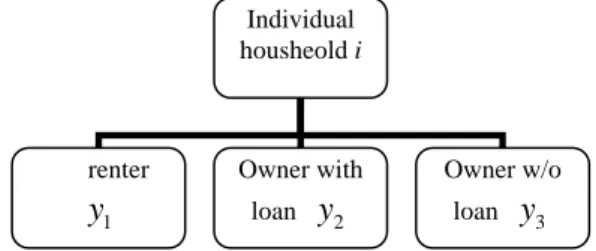
(2) Equation (2) is a standard multi-nomial logit model. There are three types of housing choice in this study: renter, owner with loan, and owner without loan. Taking renters as reference group, the relative coefficients of owners with and without loan can be estimated. In this case, the three types of choices are parallel as shown in figure 1. The above statement is hold under certain hypothesis: the independence from irrelevant alternatives (IIA), i.e., relative probability of any two choices is independent from the others, or every choice is independent from each other.

Figure 1: deicison structure of hosuing tenure choice, IIA holds.

If the IIA hypothesis does not hold, one way to deal with this is a nested logit model. In a nested logit specification, choices are ranked by order. In this study, assume the household choose owning or renting first. For owners, making loan or not is the decision afterward. The structure of decision is as figure 2: Individual houshold i Renter ,1 i

Y

Owner ,2 i

Y

Owner with loan 1 2

i

Y

Owner without loan 2 2 i

Y

Individual housheold i renter 1 y Owner with loan y₂ Owner w/o loan y₃

6

In a nested logit model, utility of individual household is expressed as:

tm t m tm t m tm

U

= +

V

V

+

V

+ +

ε ε

+

ε

, (3) where

ε ε ε

、 、

_{t m tm} are residuals.

In Equation (3),

V

_t is utility of tenure choice,

V

_m is that of choosing loan,

V

_tm is that of choosing loan and tenure choice.

ε ε ε

、 、

_{t m tm} are immeasurable in utility function that follow consistent Gumbel distribution. As such, the joint probability of choosing housing ownership and loan request of individual household i is as follows:

( )

( )

tm

P

=

P m t

⋅

P t

, (4) where P t

( )

of Equation (4) is the marginal probability of ownership while, P m t

( )

, that of loan choice. Assume the corresponding household characteristics of the tenure choice is X_{i t,} with decisions Y_{i t,} ; the corresponding household characteristics of loan taking decision is

,

i m t

X

with decision

Y

_{i m t,} . The probability of each layer is expressed as:

( )

, , , , m i m t i m t l i m t i m t X Y X Y l

e

P m t

e

β α β α + + ′

=

∑

, (5)

( )

, , , , k i t i t k k i t i t k X Y I X Y I k

e

P t

e

β α τ β α τ ′ + + + + ′

=

∑

. (6) In the two layers decision structure, estimation procedure is reverse. We have to estimate the inclusive value of loan choice probability of lower level decision before the estimation of the upper level tenure choice. The inclusive value It with estimated coefficient

τ

:

, ,

log

lXi m t Yi m t t l

I

e

β +α ′

⎛

⎞

=

_⎜

_⎟

⎝

∑

⎠

. (7)

If

τ

=1, Equation (7) degenerates to be a multi-nomial logit model; if

τ

>1 or

τ

<0, it suggests that model specification is not consistent with random utility function and it needs to be remodeled. The inclusive value therefore provides a testing criteria for the validity of nested logit model. There are two types of algorism for estimation: first is called limited information maximum likelihood (LIML) or 2 stage estimates, second is called full information maximum likelihood (FIML) which estimates parameters of Equation (5) to (7) at a time. This study uses

7

FIML procedure in estimation.

3. Data Description

This study uses the Survey of Family Income and Expenditure (SFIE) of Taiwan, conducted by the Directorate-General of Budget, Accounting and Statistics (DGBAS) in 2000 to estimate tenure choice. There are 15,159 effective samples, where 3,425 are households with two generations of income earners, and 11,714 households with one generation of income earners.

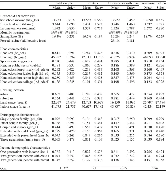
Basic statistics of overall samples and three types of households are shown in Table I. In addition to the total sample statistics, three types of households (renters, homeowners with an without loan) are separately treated. It is clear that homeowners with loan earn the most, while save the least, among three types of households. Renters have higher probability to be female headed than owners while the reverse will be true for homeowners without loan. Household size, income earners, intact couple, head in public sector and head’s education all demonstrate similar patterns between different types of housing ownership. With regard to housing location, renters tend to concentrate on urban area and homeowner without loan, rural area. Land space and indoor space also display consistent patterns between housing ownership types that renter’s housing space is smaller than others’.

8

Table 1 General Statistics, SFIE 2000

Mean Stdev Mean Stdev Mean Stdev Mean Stdev Household characteristics

household income (hhy_tot) 13.733 0.616 13.557 0.566 13.922 0.459 13.690 0.655 Household size (hhsize) 3.644 1.690 3.434 1.592 3.746 1.460 3.637 1.775 Income earners (tot_ernr) 1.672 0.850 1.537 0.773 1.726 0.787 1.672 0.880 Monthly housing loan ####### ####### ######## ########

Saving Rate (%) 16.4% 0.233 16.2% 0.199 10.2% 0.244 18.7% 0.229

Forced saving (add housing loan) 25.1% 0.181

Head characteristics

Head sex (hd_sex) 0.812 0.391 0.767 0.423 0.836 0.370 0.809 0.393 Head age (hd_age) 45.987 13.262 42.111 11.705 41.625 9.924 48.093 13.990 Spouse exist (sp_exist) 0.720 0.449 0.628 0.484 0.785 0.411 0.710 0.454 Head in public sector (public) 0.131 0.337 0.060 0.237 0.186 0.389 0.121 0.326 Head education-primary (hd_edelem 0.232 0.422 0.219 0.413 0.160 0.367 0.260 0.439 Head education-junior high (hd_edj 0.175 0.380 0.217 0.412 0.163 0.369 0.173 0.378 Head education-senior high (hd_edh 0.289 0.453 0.344 0.475 0.337 0.473 0.264 0.441 Head education-college ( hd_edcoll 0.138 0.345 0.101 0.301 0.198 0.398 0.123 0.328 Housing location

urban 0.602 0.489 0.788 0.409 0.665 0.472 0.554 0.497

suburban 0.264 0.441 0.178 0.383 0.281 0.449 0.269 0.444

Land space (area_t) 22.267 24.679 12.723 10.627 16.150 16.995 25.797 27.474 Indoor space (area_r) 41.675 21.737 30.627 17.182 43.837 20.828 42.454 22.179 Demographic characteristics

Single person family (gen_00) 0.095 0.293 0.136 0.343 0.067 0.250 0.099 0.299 Intact couple family (gen_0) 0.188 0.391 0.154 0.361 0.137 0.344 0.211 0.408 Couple and minors (gen_1) 0.414 0.493 0.552 0.497 0.593 0.491 0.330 0.470 Extended with child head (gen_2y) 0.229 0.420 0.155 0.362 0.165 0.371 0.263 0.440 Extended with parent head (gen_2o 0.075 0.263 0.049 0.216 0.053 0.225 0.086 0.280 Three generation family (gen_3) 0.033 0.179 0.011 0.103 0.025 0.155 0.039 0.194 Income demographic characteristics

One generation with income (inc_1) 0.782 0.413 0.827 0.378 0.811 0.392 0.765 0.424 Two generation income with child h 0.071 0.257 0.043 0.203 0.052 0.222 0.081 0.274 Two generation income with parent 0.145 0.352 0.129 0.336 0.136 0.343 0.151 0.358 Obs.

Total sample Renters Homeowner with loan Homeowner w/o loa

11952 1121 2855 7976

4. Regression Result

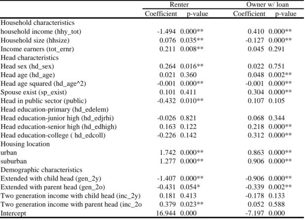
Table 2 is the result of multi-nomial logit model of tenure choice with owner without loan as the reference group. It is suggested that household income, head age, head in public sector, and extended family are negatively associated with the probability of renter while household size, income earner, male headed, urbanization, two generation with income parent headed are positively associated with renter (relative to owner without loan). For owners with loan, household income, intact couple, higher educated head are positively correlated with the

propensity to own with loan than that without. Household size and extended family are negatively correlated with. Regarding head’s age, since linear and quadratic terms are both significant, we

9

try to graph the age ownership pattern and the result is shown in graph 1.

Table 2 Multi-nomial logit of tenure choice

Coefficient p-value Coefficient p-value

Household characteristics

household income (hhy_tot) -1.494 0.000** 0.410 0.000**

Household size (hhsize) 0.076 0.035** -0.127 0.000**

Income earners (tot_ernr) 0.211 0.008** 0.045 0.291

Head characteristics

Head sex (hd_sex) 0.264 0.016** 0.022 0.751

Head age (hd_age) 0.021 0.360 0.048 0.002**

Head age squared (hd_age^2) -0.001 0.000** -0.001 0.000**

Spouse exist (sp_exist) 0.101 0.411 0.304 0.000**

Head in public sector (public) -0.432 0.010** 0.107 0.105

Head education-primary (hd_edelem)

Head education-junior high (hd_edjrhi) -0.026 0.821 0.068 0.344

Head education-senior high (hd_edhigh) 0.163 0.122 0.218 0.000**

Head education-college ( hd_edcoll) -0.226 0.142 0.312 0.000**

Housing location

urban 1.742 0.000** 0.863 0.000**

suburban 1.277 0.000** 0.906 0.000**

Demographic characteristics

Extended with child head (gen_2y) -1.407 0.000** -0.906 0.000**

Extended with parent head (gen_2o) -0.431 0.054* -0.339 0.002**

Two generation income with child head (inc_2y) 0.181 0.413 -0.178 0.133

Two generation income with parent head (inc_2o) 0.379 0.023** 0.052 0.588

Intercept 16.944 0.000 -7.197 0.000

Note: owner without loan as the reference group

Renter Owner w/ loan

Given the results of Table 2, it is needed to test the hypothesis of IIA to prove the validity of multi-nomial logit model. The result shows that IIA hypothesis is not fully supported by the results.

Table 3 IIA tests

renter vs. owner w/o loan renter vs. owner w/ loan owner w/ v.s. w/o loan

-16.970 1208.030 -21.110

p-value 0.312 0.000 0.267

conclusion not rejected rejected not rejected

2

10 Life-cycle effect -1.00 -0.80 -0.60 -0.40 -0.20 0.00 0.20 0.40 0.60 0.80 20 23 26 29 32 35 38 41 44 47 50 53 56 59

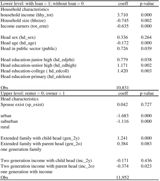
We then turn to nested logit model. As shown in Table 4, we divide the decision to be two layers: the lower level for loan demand and the upper level, tenure choice. For the lower level, income level, head in public sector and educational level are positively associated with loan tendency of the owners while household size, income earner and head age are the reverse. For tenure choice, urbanization and two generation with income are negatively associated with ownership while extended family are positively associated with.

11

Table 4 Nested logit model of tenure choice and loan choice

Lower level: with loan = 1; without loan = 0 coeff p-value Household characteristics

household income (hhy_tot) 3.710 0.000

Household size (hhsize) -0.745 0.002

Income earners (tot_ernr) -0.635 0.000

Head sex (hd_sex) 0.336 0.264

Head age (hd_age) -0.172 0.000

Head in public sector (public) 0.726 0.039

Head education-junior high (hd_edjrhi) 0.779 0.038 Head education-senior high (hd_edhigh) 1.171 0.002

Head education-college ( hd_edcoll) 1.420 0.003

Head education-primary (hd_edelem)

Obs 10,831

Upper level: renter = 0; owner = 1 coeff p-value

Head characteristics

Spouse exist (sp_exist) 0.042 0.727

urban -1.683 0.000

suburban -1.116 0.000

rural

Extended family with child head (gen_2y) 1.241 0.000 Extended family with parent head (gen_2o) 0.384 0.083 one generation family

Two generation income with child head (inc_2y) -0.171 0.436 Two generation income with parent head (inc_2o) -0.374 0.023 one generation with income

12

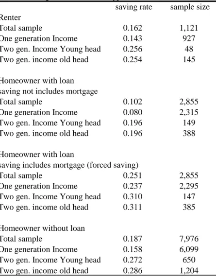
Table 5 Saving rates of different types of household

saving rate sample size

Renter

Total sample 0.162 1,121

One generation Income 0.143 927

Two gen. Income Young head 0.256 48

Two gen. income old head 0.254 145

Homeowner with loan saving not includes mortgage

Total sample 0.102 2,855

One generation Income 0.080 2,315

Two gen. Income Young head 0.196 149

Two gen. income old head 0.196 388

Homeowner with loan

saving includes mortgage (forced saving)

Total sample 0.251 2,855

One generation Income 0.237 2,295

Two gen. Income Young head 0.310 147

Two gen. income old head 0.311 385

Homeowner without loan

Total sample 0.187 7,976

One generation Income 0.158 6,099

Two gen. Income Young head 0.272 650

Two gen. income old head 0.286 1,204

Following the analysis of tenure choice, next question is saving rate of different types of housing ownership. For renter and homeowner without loan, the saving rates are similar.

Homeowners with loan tend to save less. However, if we add the loan payment (defined as forced saving) back to saving, the saving rate will be the highest among three types of household.

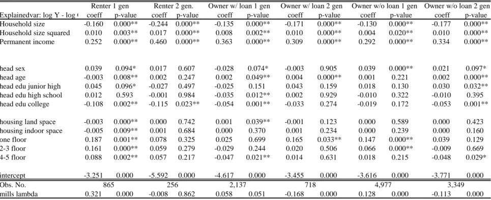
Table 6 Houeshold saving function with the consideration of Heckman correction

Explainedvar: log Y - log C coeff p-value coeff p-value coeff p-value coeff p-value coeff p-value coeff p-value

Household size -0.160 0.000** -0.244 0.000** -0.135 0.000** -0.171 0.000** -0.130 0.000** -0.177 0.000**

Household size squared 0.010 0.003** 0.017 0.000** 0.008 0.002** 0.010 0.000** 0.004 0.020** 0.010 0.000**

Permanent income 0.252 0.000** 0.460 0.000** 0.363 0.000** 0.309 0.000** 0.292 0.000** 0.334 0.000**

head sex 0.039 0.094* 0.017 0.607 -0.028 0.074* -0.003 0.905 0.039 0.000** 0.021 0.097*

head age -0.003 0.008** 0.002 0.247 0.002 0.049** 0.004 0.000** 0.001 0.221 0.002 0.000**

head edu junior high 0.045 0.096* -0.027 0.497 -0.025 0.151 0.043 0.159 0.018 0.130 0.030 0.032**

head edu high school 0.012 0.593 -0.001 0.984 -0.035 0.012** 0.002 0.929 -0.010 0.322 -0.010 0.395

head edu college -0.108 0.002** -0.115 0.023** -0.054 0.001** -0.033 0.274 -0.019 0.172 -0.053 0.001**

housing land space -0.003 0.000** 0.000 0.742 0.001 0.039** -0.001 0.123 0.000 0.589 0.000 0.423

housing indoor space -0.005 0.009** 0.001 0.684 0.000 0.370 0.001 0.234 0.000 0.239 0.000 0.160

one floor 0.187 0.001** 0.078 0.325 0.025 0.699 0.165 0.033** 0.147 0.000** 0.039 0.129 2-3 floor 0.161 0.000** 0.059 0.279 -0.029 0.244 0.020 0.506 0.066 0.000** -0.009 0.669 4-5 floor 0.088 0.002** 0.057 0.217 -0.047 0.021** 0.014 0.631 0.018 0.215 -0.048 0.029* intercept -3.251 0.000 -5.592 0.000 -4.617 0.000 -3.455 0.000 -3.616 0.000 -3.771 0.000 Obs. No. mills lambda 0.321 0.000 -0.008 0.862 0.058 0.051 -0.168 0.000 0.128 0.000 -0.113 0.000 2,137 718 4,977 3,349

Renter 1 gen Renter 2 gen. Owner w/ loan 1 gen Owner w/ loan 2 gen Owner w/o loan 1 gen Owner w/o loan 2 gen

Table 6 shows that household size is not favorable toward saving though the effects are decreasing along with size. The marginal propensity to save out of permanent income (MPS) is the highest for renters of two generation and then owners with loan of one generation. These two types of households tend to be under large pressure to save more either for home buying or loan payment. That renters of one generation tend to save the least may reflects the fact that the disadvantaged group has lower priority for housing purchase. However, it is worth to note that the MPS of one generation renter is as high as 25%. Male headed household tend to save more than female headed one except owner with loan one generation household. It is suggested that female headed one generation household (may be single person family) tend to save more than the male headed counterpart. Higher educated heads consistently save less may be associated with consumption preference. Housing space is negatively associated with renter’s saving but positively associated with that of owner with loan.

Reference

Bourassa, S. (2000). Ethnicity Endogeneity, and Housing Tenure Choice. Journal of Real Estate Finance and

Economics , pp. 323-341.

Bourassa, S. (1995). The Impacts of Borrowing Constraints on Home-Ownership in Australia. Urban

Studies , pp. 1167-1173.

Chu-Chia Lin, a. C.-L.-J. (n.d.). Life Cycle, Mortgage Payment, and Forced Savings. INTERNATIONAL

REAL ESTATE REVIEW , pp. 109-141.

Chu-Chia Lin, a. Y.-F. (2003). Housing Prices,Mortgage Payments and Savings Behavior in Taiwan: A Time Series Analysis. Asian Economic Journal , pp. 407-425.

Deaton A., a. C. (1998). Aging and Inquality in Income and Health. Amercian Economic Review , pp. 248-263.

Deaton A., a. C. (1995). Saving, Inquality and Aging：An East Asia Perspective. Asia Pacific Economic

Review , pp. 7-19.

Fumo, H. (1986). Analysis of Household Saving: Past, Persent, and Future. Japanese Economic Review , pp. 21-33.

Hsueh, L.-M. (2000). The Relationship between Housing Price, Tenure Choice and Saving Behavior in Taiwan. INTERNATIONAL REAL ESTATE REVIEW , pp. 11-33.

Lin, C.C., 1993. The relationship between rents and prices of owner-occupied housing in Taiwan. J. Real Estate Finan. Econ. 6, 25-54.

Lin, C.C., Yung, C.S., Chang, C.O., 1996. Housing price index in Taipei. J. Housing Stud. 4, 1-30 (in Chinese).

Lin C.C., Lai, Y.F., 2003. Housing price, mortgage payments and savings behavior in Taiwan: a time series analysis. Asian Econ. J. 17, 407-425.

McFadden, D. (1974). Conditional Logit Analysis of Qualitative Choice Behavior. Frontier in Econometrics , pp. 105-142.

Phang, S.-Y. (2004). House prices and aggregrate consumption: do they move together? Evidence from Singapore. Journal of Housing Economics , pp. 101-119.

Tachibanaki, T. a. (1988). Household Saving, Life Insurance, and Public Pension. Bunken Journal , pp. 23-58.

Tachibanaki, T. (1994). Housing and Saving in Japan. Housing Markets in the United States and Japan , pp. 161-190.