使用大亞灣微中子實驗探測器測量緲子散裂作用產生的中子被氫原子與釓原子俘獲之比例研究

國 立 交 通 大 學

物理研究所

碩士論文

使用大亞灣微中子實驗探測器測量緲子散裂作用產生

的中子被氫原子與釓原子俘獲之比例研究

Measurements of the Spallation Neutron Capture

Rates by Hydrogen and Gadolinium Using the

Daya Bay Detector

研究生：林秉言

指導教授：林貴林 教授

國 立 交 通 大 學

物理研究所

碩士論文

使用大亞灣微中子實驗探測器測量緲子散裂作用產生

的中子被氫原子與釓原子俘獲之比例研究

Measurements of the Spallation Neutron Capture

Rates by Hydrogen and Gadolinium Using the

Daya Bay Detector

研究生：林秉言

指導教授：林貴林 教授

使用大亞灣微中子實驗探測器測量緲子散裂作用產生的中

子被氫原子與釓原子俘獲之比例研究

Measurements of the Spallation Neutron Capture Rates by

Hydrogen and Gadolinium Using the Daya Bay Detector

研 究 生：林秉言 Student：Ping-Yen Lin

指導教授：林貴林 Advisor：Guey-Lin Lin

國 立 交 通 大 學

物 理 研 究 所

碩 士 論 文

Submitted to Institute of Physics National Chiao Tung University in Partial Fulfillment of the Requirements

for the Degree of Master

in Physics July 2014

Hsinchu, Taiwan, Republic of China

i

使用大亞灣微中子實驗探測器測量緲子散裂作用產生

的中子被氫原子與釓原子俘獲之比例研究

學生：林秉言

指導教授：林貴林

國立交通大學物理研究所

摘要

大亞灣反應堆微中子實驗是利用反 β 衰變測量反

應堆微中子的振盪，實驗以釓原子來捕捉反 β 衰變中

產生的中子，而宇宙射線緲子通過介質時所反應產生

的中子被釓原子捕捉後產生的訊號是大亞灣實驗一個

重要的背景。為了了解宇宙射線緲子導致的中子產量，

必須分析與計算中子被釓原子捕捉的數量在中子被氫

原子或釓原子捕捉的總數量中所佔之比例。我們分析

了 2011 年 12 月 24 日到 2012 年 7 月 28 日的數據，得

出了這個比例在六個探測器分別為：84.75％±0.3％

(AD1)、84.6％±0.26％(AD2)、84.67％±0.39％(AD3)、

85.11％±0.6％(AD4)、85.11％±0.56％(AD5)和 85.13

％±0.59％(AD6)。

Measurements of the Spallation Neutron Capture Rates

by Hydrogen and Gadolinium Using the Daya Bay

Detector

Student：Ping-Yen Lin

Advisor：Guey-Lin Lin

Institute of Physics

National Chiao Tung University

ABSTRACT

The Daya Bay reactor neutrino experiment measures

the reactor neutrino oscillation with the inverse beta decay,

where the neutron produced is captured by Gadolinium.

The cosmic muon-induced neutron cause the important

background for the Daya Bay experiment. To analyze the

muon-induced neutron yield, calculating the neutron

capture rates by Hydrogen and Gadolinium is essential.

We analyze the data of 6 ADs in a period of time from

December 24, 2011 to July 28, 2012. We find the rates for

each AD: 84.75％±0.3％(AD1), 84.6％±0.26％(AD2),

84.67％±0.39％(AD3), 85.11％±0.6％(AD4), 85.11％±

0.56％(AD5), and 85.13％±0.59％(AD6).

iii

誌謝

謝謝指導教授林貴林老師在我就讀碩士班期間各方面

的照顧與指導。

謝謝口試委員高文芳老師與王正祥老師寶貴的建議。

謝謝大亞灣合作組在技術和資源上的支援。

謝謝葉永順與胡貝禎在研究過程中，提供我技術上的

引導及各方面的討論與協助。

謝謝交大物理所所有人的陪伴。

謝謝張光春、陳囿任、黃清銓、梁璐、林天宇、馬守

正、姚懿恆陪我遠航。

謝謝黃昱翔與羅令崴陪伴我，鼓勵我，照顧我。

最後，謝謝我最摯愛的家人給我無條件的支持與愛

護，並且信任我，讓我可以任性的做我想做的事。

林秉言(P. Y. Lin)

2014 年夏 於國立交通大學

Contents

List of Tables vii

1 Introduction 1

1.1 Neutrino Physics . . . 1

1.2 Measurement of Electron Antineutrino . . . 4

1.3 Cosmic Muon-induced Backgrounds . . . 6

2 The Daya Bay Neutrino Experiment 8 2.1 Experiment Layout . . . 8

2.2 Detectors . . . 10

2.3 Measurement of θ13and Backgrounds . . . 12

2.3.1 Measurement of θ13. . . 13

2.3.2 Backgrounds . . . 15

3 H-Gd Ratio from Spallation Neutrons 18 3.1 Muon-induced Neutron Production . . . 18

3.2 Event Selection . . . 19

3.3 H-Gd Ratio . . . 21

3.3.1 Cut Selection . . . 23

3.3.2 Cut Efficiency . . . 32

3.3.3 Ratio, Statistical Error and Systematical Error for Each AD . . . 36

4 Conclusion 40

Bibliography 42

Appendix 44

List of Figures

1.1 The energy spectrum of β particle in theoretical calculation. . . . 2

1.2 The Feynman diagram of a muon spallation process. . . 6

2.1 Layout of the Daya Bay experiment. . . 9

2.2 Schematic of the ADs, water shields, and RPCs in near hall. . . 10

2.3 The antineutrino detector. . . 11

2.4 The MCS installed on the AD. . . 12

2.5 An RPC module structure. . . 13

2.6 Prompt IBD spectra. . . 14

2.7 Rate-only oscillation results. . . 16

3.1 A 2D map showing the time since the last muon versus the energy of the spallation products. . . 20

3.2 The time since the last muon (dT ) for each AD. . . . 21

3.3 The energy spectrum of DYB AD1 in signal time window. . . 22

3.4 The energy spectrum of DYB AD1 in background time window. . . 22

3.5 The energy spectrum after background subtraction of DYB AD1. . . 23

3.6 The mean and the sigma of the nH energy peak for AD1. . . 24

3.7 The mean and the sigma of the nGd energy peak for AD1. . . 24

3.8 The mean and the sigma of the nH energy peak for AD2. . . 25

3.9 The mean and the sigma of the nGd energy peak for AD2. . . 25

3.10 The mean and the sigma of the nH energy peak for AD3. . . 26

3.11 The mean and the sigma of the nGd energy peak for AD3. . . 26

3.12 The mean and the sigma of the nH energy peak for AD4. . . 27

3.13 The mean and the sigma of the nGd energy peak for AD4. . . 27

3.14 The mean and the sigma of the nH energy peak for AD5. . . 28

3.15 The mean and the sigma of the nGd energy peak for AD5. . . 28

3.16 The mean and the sigma of the nH energy peak for AD6. . . 29

3.17 The mean and the sigma of the nGd energy peak for AD6. . . 29

3.18 The RH-Gdversus different ranges of fiducial cut. . . 30

3.19 The RH-Gdversus various energy cuts for all ADs. . . 31

3.20 The RH-Gdversus various timing cuts for all ADs. . . 31

3.21 The ϵF nGdversus various fiducial cuts. . . 33

3.22 The ϵF nH versus various fiducial cuts. . . 34

3.23 The ϵT nGdversus various timing cuts. . . 34

3.24 The ϵT nH versus various timing cuts. . . 35

3.25 The ϵEnGdversus various energy cuts. . . 35

3.26 The ϵEnH versus various energy cuts. . . 36

3.28 The R′_H-Gdversus various fiducial cuts. . . 38 3.29 The R′_H-Gdversus various timing cuts. . . 38 4.1 The H-Gd ratio with statistical error and systematical error for each AD. 41

List of Tables

1.1 The Gd-capture ratio using two different methods in Ref. [10]. . . 7

2.1 Site information including baselines and overburdens. D1/D2, L1/L2, and L3/L4 stand for the reactor cores. . . 9

2.2 Lists of calibration sources. . . 11

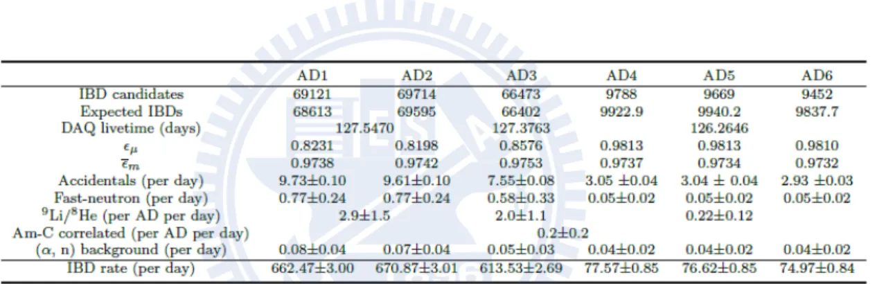
2.3 Summary of signal and background in ADs in the 3 EHs. . . 17

3.1 The R′_H-Gdand σ′_statof energy cuts for each AD. . . 36

3.2 The R′_H-Gdand σ′_statof fiducial cuts for each AD. . . 37

3.3 The R′_H-Gdand σ′_statof timing cuts for each AD. . . 37

Chapter 1

Introduction

1.1

Neutrino Physics

In 1930, Pauli proposed a new particle in order to explain the conservation law of energy-momentum and spin angular energy-momentum in the β-decay experiment [1]. Two-body decay model of the β-decay is that a neutron decay into a proton and an electron (β particle). The emitted electron should have a fixed energy which contradict with the continuous energy spectrum in β-decay experiment by J. Chadwick in 1914 [2]. Pauli indicated that the new particle, named neutrino, is a neutral and extremely light fermion in the final state of β-decay. The spectrum of β-decay can be calculated theoretically [3] by dΓ dE = 1 π3~ ( gw 2MWc2 )4 E√E2− m2 ec4 [ (mn− mp)c2− E ]2 , (1.1)

where Γ, E, gw, MW, me, mn and mp are total decay rate, energy of electron, weak

re-Figure 1.1: The energy spectrum of β particle in theoretical calculation.

Neutrino was first detected by Cowan and Reines in 1956 by the inverse β-decay process [4]

νe+ p−→ e++ n , (1.2)

where the antineutrino was produced in a reactor. In 1962, L. Lederman, M. Schwartz, and J. Steinberger discovered the muon neutrino νµin Brookhaven National Laboratory

[5]. The tau neutrino ντ was observed by Fermi National Accelerator Laboratory in

2000 [6].

In the late 1960s, it was found that the number of electron neutrino from Sun in the Homestake experiment are different from the number predicted by standard solar model [7]. The experimental number is only 1/3 of the theoretical prediction. This is so-called the solar neutrino problem. In 2001, the result of the SUDBURY Neutrino Observatory (SNO) experiment directly demonstrated the neutrino oscillation effect which implied that neutrinos are massive.

The problem of neutrino oscillation is that neutrino weak eigenstates do not correspond to the neutrino mass eigenstates, but are mixture of each other. Neutrinos interact in their flavor eigenstates, but they propagate in the mass eigenstates. The transformation relating the flavor and mass eigenstates can be written as

|να⟩ = α

∑

i

Uαi|νi⟩ , (1.3)

where|να⟩ and |νi⟩ represent the flavor eigenstates and the mass eigenstates of neutrino

with α = e, µ, τ and i = 1, 2, 3, respectively. Uαiis the Pontecorvo–Maki–Nakagawa–

Sakata (PMNS) mixing matrix. For three neutrino flavors, the PMNS matrix is a 3×3 unitary matrix. U =         Ue1 Ue2 Ue3 Uµ1 Uµ2 Uµ3 Uτ 1 Uτ 2 Uτ 3         =         1 0 0 0 C23 S23 0 −S23 C23                 C13 0 S13eiδ 0 1 0 −S13eiδ 0 C13                 C12 S12 0 −S12 C12 0 0 0 1         ×         eiα1/2 _{0 0} 0 eiα2/2 ₀ 0 0 1        

=         C12C13 S12C13 S13e−iδ −S12C23− C12S23S13eiδ C12C23− S12S23S13eiδ S23C13 S12S23− C12C23S13eiδ −C12S23− S12C23S13eiδ C23C13         ×         eiα1/2 _{0 0} 0 eiα2/2 ₀ 0 0 1         , (1.4)

where Uαiis the element of transition matrix from the mass eigenstates|νi⟩ to the flavor

eigenstates|να⟩, Sij and Cij are sin θij and cos θij with θij the mixing angle between i

and j mass eigenstate. δ, α1 and α2 are the CP phase and Majorana phases.

1.2

Measurement of Electron Antineutrino

The antineutrino is produced by the reactors of Daya Bay nuclear power complex. There are two near sites and one far site with eight antineutrino detectors (ADs). Two ADs are placed at each near site. Four ADs are placed at the far site for increasing the statistics. The survival probability of antineutrino was measured in order to obtain θ13. The

sur-vival probability for electron antineutrino in vacuum with an energy E at a distance L is given by Psur = Pee=|⟨νe|νe(t)⟩|2 = 1− sin22θ13sin2 ∆m2 31L 4Eν − cos4_θ 13sin22θ12sin2 ∆m2 21L 4Eν (1.5)

is given by Nf Nn = ( Np,f Np,n ) ( Ln Lf )2( ϵf ϵn ) [ Psur(E, Lf) Psur(E, Ln) ] , (1.6)

where index f and n are for far site and for near site respectively. N , Np, L, and ϵ are

measured rates, detector mass, distance to reactor, and detector efficiency, respectively.

E and Lf (Ln) in Psur correspond to Eν and L in Eq. (1.5) respectively. And the value

of sin22θ13is approximatiely given by

sin22θ13 ≈ 1 A(E, Lf) [ 1− ( Nf Nn ) ( Lf Ln )2] (1.7)

where A(E, Lf) = sin2 ∆31with ∆31≡ 1.267 ∆m231(eV

2_)×103 L(km)

E(MeV)and ∆m

2 31≡

m2₃− m2₁.

The antinutrino is detected by the inverse β-decay process in Daya Bay experiment [8]. There are two kinds of gamma ray signals for antineutrino measurement. The first signal produced by positron which is annihilated immediately, called prompt signal. A neutron is captured by proton or Gd nucleus that produced the so-call delay signal comparing to the prompt one. If the neutron is captured by a proton, a 2.2MeV gamma-ray is emitted for each event [8],i.e.

n + p−→ D + γ(2.2MeV ) (1.8)

In order to increase the neutron capture probability, a 0.1% Gd was doped in the liquid scintillator (LS) in AD. The Gd was excited by captured neutrons and returned to the

ground state by emitting 8 MeV gamma [8, 9].

n + Gd−→ Gd∗ (1.9)

Gd∗ −→ Gd + γ(8MeV ) (1.10)

The delayed signal efficiently tags antineutrino signal. The prompt and the delayed coincidence provides a distinctive signature.

1.3

Cosmic Muon-induced Backgrounds

It is important to understanding the cosmogenic backgrounds for underground experi-ments. Cosmic-ray muons produce neutrons through the following mechanisms [10],

• Photo-nuclear reactions: Muons generate electromagnetic shower by Photo-nuclear reactions [11].

• Muon Spallations: Muon exchange a virtual photon with nuclei and then a neu-tron is produced. Figure 1.2 shows the lowest-order Feynman diagram for this interaction.

Figure 1.2: The Feynman diagram of a muon spallation process.

• Secondary neutrons: The neutron production from the other neutrons produced by above processes.

• µ−capture on nuclei: Neutrons are produced by a low energy µ−which undergoes nuclear capture via the weak charged-current process,

µ−+ A (Z, N )−→ νµ+ A (Z− 1, N + 1) (1.11)

Neutron yield is very important for neutron background estimation. The determina-tion of the spalladetermina-tion neutron capture rates by Hydrogen and Gadolinium is essential for measuring the muon-induced neutron yield. The neutron yield depends on the average muon energy. We are interested in whether the H-Gd ratio also depends on the average muon energy. In previous studies by Yung-Shun Yeh, the ratio has been investigated using simulation data [10]. Table 1.1 shows his results. Here, we analyze the H-Gd cap-ture ratio using the experimental data. The purpose of this thesis is to measure spallation neutron capture rates by Hydrogen and Gadolinium in the Daya Bay experiment.

Table 1.1: The Gd-capture ratio using two different methods in Ref. [10], where ϵGdand

Chapter 2

The Daya Bay Neutrino Experiment

The Daya Bay experiment measures the rates and energy spectra of reactor electron antineutrinos at different baselines to estimate the mixing angle θ13with a sensitivity of

0.01 or better in sin2_2θ

13at 90% confidence level.

2.1

Experiment Layout

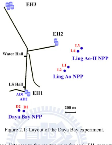
The Daya Bay Experiment [12] is located at the Daya Bay nuclear power complex in southern China. There are three nuclear power plants (NPPs) in the Daya Bay nuclear power complex: the Daya Bay NPP, the Ling Ao NPP and the Ling Ao II NPP. Each NPP consists of two reactor cores. The layout of the Daya Bay experiment are shown in Figure 2.1. All six cores are functionally identical reactors of 2.9 GW thermal power [12]. It gives a prolific source of reactor antineutrinos (∼ 6 × 1020νe/s/core).

There are three experimental halls (EHs) in the Daya Bay experiment: the Daya Bay near hall (EH1) and the Ling Ao near hall (EH2), and one far hall (EH3). All experi-mental halls are underground. There are mountains providing overburden to suppress cosmogenic backgrounds. Table 2.1 shows the overburden, muon rate, average muon

Figure 2.1: Layout of the Daya Bay experiment.

energy, and average distances to the reactor pairs for each EH, respectively. Each

an-Table 2.1: Site information including baselines (in meters) and overburdens. D1/D2, L1/L2, and L3/L4 stand for the reactor cores and Figure 2.1 shows the layout.

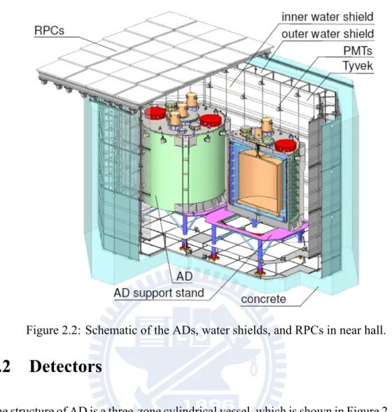
tineutrino detector (AD) is put in a water pool. The water pool shields backgrounds from the surrounding and as a detector of Cherenkov to tag cosmic-ray muons. On the top of the water pool, the resistance plate chambers (RPCs) gives an additional muon-tagging. Figure 2.2 shows the schematics of near hall. There is a similar layout with a larger water pool and RPC module array in the far hall.

Figure 2.2: Schematic of the ADs, water shields, and RPCs in near hall.

2.2

Detectors

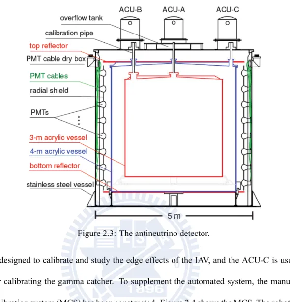
The structure of AD is a three-zone cylindrical vessel, which is shown in Figure 2.3. The innermost acrylic vessel (IAV) with diameters about 3 m is filled with about 20 tons of 0.1%-doped Gadolinium liquid scintillator (GdLS) as the target region. The medium zone between IAV and the outer acrylic vessel (OAV) with diameters about 4 m is filled with about 20 tons of pure liquid scintillator (LS) to capture gamma rays escaping from the target region. There are 37 tons of Mineral oil (MO) filled in the outermost zone , between the OAV and the stainless steel vessel (SSV) with diameters about 5 m, in order to avoid the entering of external radiation. All 192 8-inch photomultiplier tubes (PMTs) are installed in 8 rows (rings) and 24 columns on the inner wall of SSV with rails.

There are three Automated Calibration Units (ACUs) installed on the top of the AD as shown in Figure 2.3. The ACU-A sits on the central axis of the AD. The ACU-B

Figure 2.3: The antineutrino detector.

is designed to calibrate and study the edge effects of the IAV, and the ACU-C is used for calibrating the gamma catcher. To supplement the automated system, the manual calibration system (MCS) has been constructed. Figure 2.4 shows the MCS. The robotic arm of MCS could put the sources at any location inside the target volume through ACU-A penetration. Table 2.2 summarizes the properties of the calibration sources in ACU-ACU and MCS.

Table 2.2: Lists of calibration sources. (*) indicates the energy of capture gammas.

Figure 2.4: The MCS installed on the AD.

the water Cherenkov detector and the Resistive Plate Chamber detector.

To shield backgrounds from the surrounding rocks and serve as a water Cherenkov detector to tag cosmic-ray muons, the ADs is surrounded by a buffer of water with a thickness of at least 2.5 m in all directions. The water pool is divided into two parts, the inner water shield (IWS) and the outer water shield (OWS). There are 288 8-inch PMTs installed in each near hall, and 384 in the far hall.

Each water pool is covered with an array of RPC module. 54 modules are installed in both of the near halls, and 81 in the far hall. The structure of RPC is shown in Figure 2.5.

2.3

Measurement of θ

and Backgrounds

The first observation of θ13with a significance of 5.2 standard deviations was reported

Figure 2.5: An RPC module structure.

±0.005 (syst.) was given by Ref. [13].

2.3.1

Measurement of θ

According to the no-oscillation assumption, the νespectrum in the far hall can be

pre-dicted by a weighted combination of the two near hall measurements. The ratio R is defined as R = Mf/ Nf, where Mf and Nf are the measured and predicted event rates

in the far hall (sum of ADs), respectively. The ratio at the far hall was [13]

R = 0.944± 0.007 (stat.) ± 0.003 (syst.) . (2.1)

The energy spectra of the prompt signal and the ratio R in far hall are shown in Fi-gure 2.6.

Figure 2.6: Top: measured prompt energy spectrum of the far hall (sum of ADs) com-pared with the no-oscillation prediction based on the measurements of the near halls. Bottom: the ratio of measured and predicted spectrum. Red solid curve is the best-fit of ratio with sin22θ13= 0.089, whereas the dashed curve is the non-oscillation prediction.

uncertainties defined as χ2 = 6 ∑ d=1 [ Md− Td ( 1 + ε +∑_rωd_rαr+ εd ) + ηd ]2 Md+ Bd +∑ r α2 r σ2 r + 6 ∑ d=1 ( ε2 d σ2 d + η 2 d σ2 B ) , (2.2)

where Mdis the measured IBD event number of the d-th AD with its backgrounds

sub-tracted, Bdis the corresponding background, Tdis the prediction from antineutrino flux,

including MC corrections and neutrino oscillations, ω_rdis the fraction of IBD contribu-tion of the r-th reactor to the d-th AD determined by the baselines and antineutrino fluxes. The uncorrelated reactor uncertainty is σr (0.8%). The parameter σd (0.2%) is

the uncorrelated detection uncertainty. The parameter σB is the quadratic sum of the

background uncertainties listed in Table 2.3. The corresponding pull parameters are (αr, εd, ηd). The detector- and reactor-related correlated uncertainties are not included

in the analysis. The absolute normalization ε was determined from the fitting to the data. The survival probability of νeused in the χ2 is

Psur = 1− sin22θ13sin2

( 1.267 ∆m2₃₁L E ) − cos4_θ 13sin22θ12sin2 ( 1.267 ∆m2₂₁L E ) , (2.3) where ∆m2 31 = 2.32× 10−3eV 2_{, sin}2 2θ12 = 0.861+0.026_−0.022, and ∆m221 = 7.59 +0.20 −0.21 × 10−5eV2 [14]. The uncertainty of ∆m2

31[15] is not included in the fitting. The best-fit

value of sin22θ13with a χ2/NDF of 3.4/4 [13] is

sin22θ13= 0.089± 0.010(stat.) ± 0.005(syst.) . (2.4)

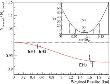
All best estimates of pull parameters are within the one standard deviation based on the corresponding systematic uncertainties. The no-oscillation hypothesis is excluded at 7.7 standard deviations. Figure 2.7 shows the number of IBD candidates in each detector after corrections for relative efficiency and background, relative to those expected as-suming no oscillation. A ∼ 1.5% oscillation effect appears in the near halls, largely due to oscillation of the antineutrinos from the reactor cores in the farther cluster. The oscillation survival probability at the best-fit values is given by the smooth curve. The

χ2 _{value versus sin}2_2θ

13is shown in the inset.

2.3.2

Backgrounds

The experiment mainly has two kinds of background, the accidental coincidence and the cosmogenic background. Below are the major backgrounds to the IBD selections:

Figure 2.7: Top: Ratio of measured versus expected signals in each detector, assuming no oscillation.

correlated signals that satisfy the IBD selection criteria accidentally.

• Fast neutron background: The energetic neutrons induced by cosmic-ray muons entering the AD could mimic the prompt signal by recoiling off a proton, and give a delayed signal after being captured on Gd.

• 9Li/8He background: The rate of correlated background from the β-n cascade

of the cosmogenic9_Li/8_{He can be estimated by evaluating the time distribution}

since the last muon.

• 1_{3C(α; n)}1_{6O background: The}1_{3C(α; n)}1_{6O background is determined by}

mea-suring α-decay rate in situ and then calculate the neutron yield by MC.

• Calibration source Am-C induced background: During the data taking, neutrons from the Am-C calibration source stored inside the ACU may mimic IBD events by scattering inelastically with nuclei in the shielding material, and captured on Fe, Cr, Mn or Ni in the stainless steel tank.

Chapter 3

H-Gd Ratio from Spallation Neutrons

In this Chapter, we determine the ratio of the muon-induced neutrons captured by Hy-drogen and those captured by Gadolinium in the GdLS region in the 3 experimental halls of the Daya Bay experiment.

3.1

Muon-induced Neutron Production

Neutrons can be produced by the interaction between muon and the surrounding matter when a cosmic-ray muon passes through the AD. Neutrons are produced by five kinds of processes: (i) photo-nuclear interactions, (ii) muon Spallations, (iii) elastic scattering, (iv) secondary neutrons, and (v) µ−capture on nuclei. When a neutron is captured on Gd (nGd in short), it releases gamma-rays with the total energy of about 8 MeV, whereas a neutron captured on H (nH) emits the gamma-ray with the characteristic energy about 2.2 MeV.

In order to determine the muon-induced neutron yield, it is necessary to convert the number of nGd events to the number of total neutron capture events in GdLS [10]. Hence we evaluate the ratio in this study.

3.2

Event Selection

The analysis is based on the data taken from December 24, 2011 to July 28, 2012. The data of 6 ADs deployed in 3 EHs is used. In this study, events are identified as cosmic-ray muons passing through the AD by the following selection criteria,

• AD muon (µAD): the energy deposit is greater than 20 MeV;

• WP muon (µWP): either the number of fired PMTs in IWS or OWS are greater

than 12;

• µAD and µWPare within 0.3 µs.

A small number of AD PMTs spontaneously emit light due to discharge within the base. These instrumental backgrounds are referred to as flasher events.

After applying the flasher cut, events fulfilling the following criteria are selected as candidates for spallation neutrons captured on Gd,

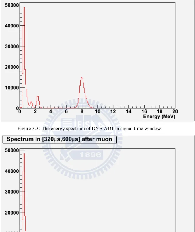
• the time since the last muon (dT ) must be located in the signal time window 20 µs < dT < 300 µs, and

• the energy range is 3 sigma region around the 8 MeV peak.

• The events within|Z| < 700 mm and R (=√X2_{+ Y}2_{) < 700 mm.}

Any event fulfilling the following criteria is selected as the candidate for spallation neu-tron captured on H,

• the time since the last muon (dT ) must be located in the signal time window that is defined as 20 µs < dT < 300 µs, and

• The events within|Z| < 700 mm and R (=√X2_{+ Y}2_{) < 700 mm.}

The lower timing cut at 20 µs is set for suppressing the effect of retrigger and ringing at the very beginning of the time period after the passing of muon[10], as depicted in Figure 3.1.

Figure 3.1: A 2D map showing the time since the last muon versus the energy of the spallation products[10].

To remove the background due to accidental coincidences, the background time win-dow is chosen as 320 µs < dT < 600 µs. Figure 3.2 shows the time since the last muon (dT ), which justifies the selection of the signal time window and the background time window.

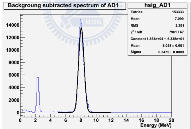
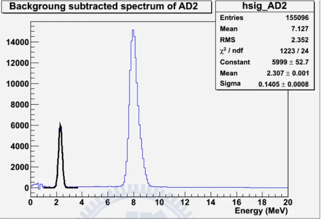
By subtracting events in the background time window from those in the signal time window (side-band subtraction in short), the accidental background can be eliminated. Figure 3.3 to Figure 3.5 show the energy spectrum in signal time window, background time window, and the energy spectrum after background subtraction, respectively.

To prevent spallation products from other muons falling on the signal time window, an isolation cut is applied such that there are no additional muon events (µAD or µWP)

Figure 3.2: The time since the last muon (dT ) for each AD. AD1 and AD2 are deployed in Daya Bay near hall, whereas AD3 is deployed in Ling Ao near hall, and the AD4 to AD6 are deployed in far hall.

3.3

H-Gd Ratio

The H-Gd ratio (RH-Gd) is defined as

RH-Gd = NGd Ntotal = NGd NH+ NGd , (3.1)

Figure 3.3: The energy spectrum of DYB AD1 in signal time window.

Figure 3.5: The spallation neutron energy spectrum of DYB AD1 with a fiducial cut of radius and height less than 700 mm. The peak around 2 MeV is neutron captured by hy-drogen and the peak around 8 MeV is neutron captured by Gd. Red histogram indicates the energy spectrum for total events before background subtraction. Green histogram in-dicates the energy spectrum in background time window, and the blue histogram shows the energy spectrum after the background subtraction.

The integrated energy range is 3 sigma around the peak. Figure 3.6 to Figure 3.17 show the mean and the sigma of the nH energy peak and the nGd energy peak for each AD separately.

3.3.1

Cut Selection

The ratio RH-Gd is affected by three cuts, which are fiducial cut (or vertex cut), energy

cut, and timing cut. The fiducial cut (F in short) involves two parameters, vertex Z and

R (= √X2_{+ Y}2_{). Figure 3.18 shows the ratio R}

H-Gd with various ranges of fiducial

cut for all ADs. The energy cut (E in short) determines the range of the Gd-capture peak and the capture peak. We adjusted the range of the Gd-capture peak and the

H-Figure 3.6: The mean and the sigma of the nH energy peak for AD1.

Figure 3.8: The mean and the sigma of the nH energy peak for AD2.

Figure 3.10: The mean and the sigma of the nH energy peak for AD3.

Figure 3.12: The mean and the sigma of the nH energy peak for AD4.

Figure 3.14: The mean and the sigma of the nH energy peak for AD5.

Figure 3.16: The mean and the sigma of the nH energy peak for AD6.

capture peak simultaneously from 2.5 sigma to 3.5 sigma. The timing cut (T in short) decides the signal time window. The width of the signal time window is kept constant (280 µs) while the beginning of the signal time window is shifted by 1 µs each time and the background time window is moved accordingly.

Figure 3.18: The RH-Gd versus different ranges of fiducial cut. Vertex means |Z| <

vertex and R < vertex.

Only one cut out of three is adjusted at once. Namely, when the energy cut is ad-justed, the other two cuts are maintained according to the criteria in Section 3.2. We show the results of various energy cuts and timing cuts in Figure 3.19 and Figure 3.20, respectively.

In the plots, the statistical error (σstat) is calculated by

σstat=

√

RH-Gd(1− RH-Gd)

Ntotal

, (3.2)

Figure 3.19: The RH-Gd versus various energy cuts for all ADs.

3.3.2

Cut Efficiency

We have calculated different cut efficiencies by Monte Carlo (MC) method (the data was produced by Yung-Shun Yeh[10]). For all cut selections, we considered the efficiency of nGd and of nH separately.

The cut efficiency of the fiducial cut (ϵF nGd and ϵF nH) are defined as follows,

ϵF nGd =

Number of nGd with fiducial cut

Number of nGd in GdLS (3.3)

and

ϵF nH =

Number of nH with fiducial cut

Number of nH in GdLS . (3.4)

Similarly, the other cut efficiency can be defined as follows

ϵT nGd =

Number of nGd with timing cut in GdLS

Number of nGd in GdLS (3.5)

ϵT nH =

Number of nH with timing cut in GdLS

Number of nH in GdLS (3.6)

ϵEnGd=

Number of nGd with energy cut in GdLS

Number of nGd in GdLS (3.7)

ϵEnH =

Number of nH with energy cut in GdLS

Number of nH in GdLS . (3.8)

Then, we define the new ratio R′_H-Gd with cut efficiency ϵGd (= ϵF nGd × ϵT nGd ×

ϵEnGd) and ϵH (= ϵF nH × ϵT nH × ϵEnH) instead of the RH-Gd as

R′_H-Gd = NGd ϵGd NGd ϵGd +NH ϵH . (3.9)

Figure 3.21: The ϵF nGdversus various fiducial cuts.

We also redefine the σstatwith cut efficiency as

σ′_stat= R′_H-Gd(R′_H-Gd− 1) √ 1 NH + 1 NGd . (3.10)

The derivation of σ′_statis shown in Appendix A. Figure 3.27 to Figure 3.29 and Figure 3.1 to Figure 3.3 show results of R′_H-Gdand σ′_stat.

Figure 3.22: The ϵF nH versus various fiducial cuts.

Figure 3.24: The ϵT nH versus various timing cuts.

Figure 3.26: The ϵEnH versus various energy cuts.

Table 3.1: The R′_H-Gd and σ_stat′ of energy cuts for each AD.

3.3.3

Ratio, Statistical Error and Systematical Error for Each AD

We already obtained 66 sets of the R′_H-Gd and the σ_stat′ for each AD. Then, we use 11 sets of data for each cut selections for each AD to get systematical error for energy cut, fiducial cut, and timing cut.

Table 3.2: The R′_H-Gd and σ_stat′ of fiducial cuts for each AD.

Table 3.3: The R′_H-Gd and σ_stat′ of timing cuts for each AD.

Figure 3.28: The R′_H-Gdversus various fiducial cuts.

called R′_mean. Then we define the σsysF, σsysE, and σsysTas σsys = v u u t 1 10 11 ∑ i=1 (R′_H-Gd− R′_mean)2, (3.11)

and define the σsyst=

√ (σsysF) 2 + (σsysE) 2 + (σsysT) 2

. Table 3.4 shows the result.

Table 3.4: The σsysF, σsysE, σsysT, and σsystfor each AD.

The ratio and the statistical error for each AD are R′_H-Gd and σ′_statwhich satisfy the criteria in Section 3.2.

Chapter 4

Conclusion

We analyzed and calculated the H-Gd ratio, cut efficiency, statistical error, and system-atical error for 6 ADs in Daya Bay experiment. The following is the results of the H-Gd ratio (R)

RAD1 = 84.75%± 0.10%(stat.) ± 0.20%(syst.) (4.1)

RAD2 = 84.60%± 0.10%(stat.) ± 0.16%(syst.) (4.2)

RAD3 = 84.67%± 0.11%(stat.) ± 0.28%(syst.) (4.3)

RAD4 = 85.11%± 0.31%(stat.) ± 0.29%(syst.) (4.4)

RAD5 = 85.11%± 0.31%(stat.) ± 0.25%(syst.) (4.5)

RAD6 = 85.13%± 0.31%(stat.) ± 0.28%(syst.) (4.6)

Figure 4.1 shows the H-Gd ratio with statistical error and systematical error for each AD. In this study, the H-Gd ratio and the average muon energy do not have significant correlations. Such a non-correlation agrees well with the result of Ref. [10].

Bibliography

[1] W. Pauli, Camb. Monogr. Part. Phys. Nucl. Phys. Cosmol. 14, 1 (2000). [2] J. Chadwick, Verh. Phys. Gesell. 16, 383 (1914).

[3] D. Griffiths, Weinheim, Germany: Wiley-VCH (2008) 454 p.

[4] F. Reines, C. L. Cowan, F. B. Harrison, A. D. McGuire and H. W. Kruse, Phys. Rev. 117, 159 (1960).

[5] G. Danby, J. M. Gaillard, K. A. Goulianos, L. M. Lederman, N. B. Mistry, M. Schwartz and J. Steinberger, Phys. Rev. Lett. 9, 36 (1962).

[6] K. Kodama et al. [DONUT Collaboration], Phys. Lett. B 504, 218 (2001).

[7] B. T. Cleveland, T. Daily, R. Davis, Jr., J. R. Distel, K. Lande, C. K. Lee, P. S. Wildenhain and J. Ullman, Astrophys. J. 496, 505 (1998).

[8] F. P. An et al. [Daya Bay Collaboration], Nucl. Instrum. Meth. A 685, 78 (2012). [9] Daya Bay collaborators, Technical Design Review, second edition, 2008.

[10] Yung-Shun Yeh, Measurement of the Neutron Yield Induced by Cosmic Muon in

the Daya Bay Reactor Neutrino Experiment , PhD thesis, National Chiao-Tung

University, 2014.

[11] Y. F. Wang, V. Balic, G. Gratta, A. Fasso, S. Roesler and A. Ferrari, Phys. Rev. D

64, 013012 (2001).

[12] X. Guo et al. [Daya-Bay Collaboration], hep-ex/0701029.

[13] F. P. An et al. [Daya Bay Collaboration], Chin. Phys. C 37, 011001 (2013). [14] B. Aharmim et al. [SNO Collaboration], Phys. Rev. C 81, 055504 (2010). [15] P. Adamson et al. [MINOS Collaboration], Phys. Rev. Lett. 106, 181801 (2011). [16] Gaosong Li, Jianglai Liu, Absolute H-Gd Ratio Study with Spallation/AmC

Neu-trons , Daya Bay Doc-7273, 2012.

[17] Bryce Littlejohn, Center HGd Ratios from Spallation Neutrons: Redux for P12E , Daya Bay Doc-9271, 2013.

[18] Feihong Zhang, H-Gd ratio study with spallation neutron , Daya Bay Doc-7554, 2012.

Appendix A

The Derivation of σ

_stat

′

The ratio R′_H-Gd with cut efficiency is defined as

R′_H-Gd = NGd ϵGd NGd ϵGd + NH ϵH = N ′ Gd N_Gd′ + N_H′ , (A.1) and 1 R′_H-Gd = 1 + N_H′ N_Gd′ (A.2) N_H′ N_Gd′ = 1 R′_H-Gd − 1 = NH NGd ϵGd ϵH (A.3) δN ′ H N_Gd′ = δ NH NGd ϵGd ϵH = ϵGd ϵH δNH NGd = δ 1 R′_H-Gd = −δR′ H-Gd R_H-Gd′ 2 (A.4)

−δR′ H-Gd = ϵGd ϵH R′_H-Gd2δNH NGd (A.5) let NH NGd = Z (A.6) δNH= √ NH (A.7) δNGd= √ NGd (A.8) thus δZ Z = √( δNH NH )2 + ( δNGd NGd )2 = √ 1 NH + 1 NGd (A.9) −δR′ H-Gd = ϵGd ϵH R_H-Gd′ 2 NH NGd √ 1 NH + 1 NGd = R_H-Gd′ 2 N ′ H N_Gd′ √ 1 NH + 1 NGd = R_H-Gd′ 2 ( 1 R′_H-Gd − 1 ) √ 1 NH + 1 NGd = R_H-Gd′ (1− R′_H-Gd) √ 1 NH + 1 NGd (A.10)

δR′_H-Gd = R′_H-Gd(R′_H-Gd− 1) √ 1 NH + 1 NGd = σ′_stat. (A.11)