使用效度與信度來比較艾菲爾微陣列基因晶片的預處理方法與表現量差異方法的組合

國 立 交 通 大 學

統計學研究所

碩 士 論 文

使用效度與信度來比較艾菲爾微陣列基因晶片的

預處理方法與表現量差異方法的組合

Validity and Reliability of Combinations of

Preprocessing and Differential Expression Methods for

Affymetrix GeneChip Microarrays

研 究 生：王雅莉

指導教授：黃冠華 博士

使用效度與信度來比較艾菲爾微陣列基因晶片的

預處理方法與表現量差異方法的組合

Validity and Reliability of Combinations of

Preprocessing and Differential Expression Methods for

Affymetrix GeneChip Microarrays

研 究 生：王雅莉 Student: Ya-Li Wang

指導教授：黃冠華 Advisor: Dr. Guan-Hua Huang

國 立 交 通 大 學

統計學研究所

碩 士 論 文

A Thesis

Submitted to institute of Statistics College of Science

National Chiao Tung University in Partial Fulfillment of the Requirements

for the Degree of Master

in Statistics July 2007

Hsinchu, Taiwan, Republic of China

使用效度與信度來比較艾菲爾微陣列基因晶片的

預處理方法與表現量差異方法的組合

研究生：王雅莉 指導教授：黃冠華 博士

國立交通大學統計學研究所

摘要

微陣列晶片的技術已被廣泛地應用了好幾年，許多計算分析的工具也已被發 展出來，而我們著重的平臺是已被廣泛應用的艾菲爾(Affymetrix)公司所製造的 基因晶片。為了評估各種預處理方法與表現量差異方法組合的表現，我們考慮了 四種常用的預處理方法：MAS 5.0、RMA、dChip 及 PDNN，與五種常用的表現 量差異方法：fold-change、two sample t-test、SAM、EBarrays 及 limma。為了評 估各種方法組合的效度，我們使用了三組嵌釘(spike-in)資料以及接收器運作指標 曲線來做評估；而為了評估信度，我們採用另一組來自「微陣列晶片品質管制計 畫」的資料組，此資料是將樣本分送至兩個同樣使用艾菲爾晶片平台的不同檢測 站所生成的資料，用此兩檢測站的資料所選出的表現量差異基因的重複率作為比 較信度的準則。若同時注重信度與效度，我們推薦幾種方法組合：當表現量差異 基因個數少時，推薦 RMA+fold-change、RMA+SAM、RMA+limma、PDNN+ fold-change、PDNN+SAM 與 PDNN+limma 此六種組合；而當表現量差異基因個 數多時，則推薦 dChip(PM-only)+fold-change、dChip(PM-only)+SAM 與 dChip(PM-only)+limma 此三種組合。 關鍵字：微陣列晶片、艾菲爾基因晶片、接收器運作指標曲線

Validity and Reliability of Combinations of

Preprocessing and Differential Expression Methods for

Affymetrix GeneChip Microarrays

Student: Ya-Li Wang Advisor: Dr. Guan-Hua Huang

Institute of Statistics

National Chiao Tung University

ABSTRACT

Microarray technology has been widely used for several years and a large number of computational analysis tools have been developed. We focus on the most popular platform, Affymetrix GeneChip arrays. To evaluate which combinations of preprocessing and differential expression method perform well, we consider 4 popular preprocessing methods (MAS 5.0, RMA ,dChip and PDNN) and 5 popular differential expression methods (fold-change, two sample t-test, SAM, EBarrays and limma). We use three spike-in datasets to assess the validity, and ROC curves are used for the evaluation. To evaluate the reliability, we use another dataset from MAQC project, which was generated using samples hybridized to Affymetrix platform at two different test sites. Overlap rates between two test sites are compared. To give consideration to both validity and reliability, six combinations are recommended when differentially expressed genes are less, RMA+fold-change, RMA+ SAM, RMA+ limma, PDNN+ fold-change, PDNN+SAM, and PDNN+limma. Three combinations are recommended when differentially expressed genes are more, dChip(PM-only)+ fold-change, dChip(PM-only)+SAM, and dChip(PM-only)+limma.

誌 謝

這兩年，真的是酸甜苦辣樣樣來，精采的兩年、快樂的兩年、辛苦的兩年、 充實的兩年！特別感謝黃冠華老師在這兩年的指導，我老是無預警地跑去找您 Meeting，甚至有時只是一件我不能確定的小事，但忙碌的您總是先放下手邊的 工作來替我解決問題與疑惑，謝謝老師的包容與耐心指導，我才能夠順利地完成 這篇論文；也謝謝老師所給的訓練，讓我寫論文的這一年來收穫良多，也過得很 充實。另外，還要感謝所上其他老師們的教導，讓我對統計有更深入的瞭解。 此外特別感謝泰賓學長以及雪芳對於我論文及程式上的指導，謝謝你們的教 導與幫忙我才能順利完成我的程式；也謝謝同門的素梅與阿淳一路來的鼓勵與支 持，忍受我壓力大時的鬼叫鬼叫，因為有你們的陪伴，我才能撐過這辛苦的一年， 很高興有你們一起奮鬥到最後，我最好的夥伴們！還有一起待在嚴寒的電腦室奮 鬥的美惠及柯柯，有你們的陪伴、打氣與取暖，我才不至於凍僵在電腦室；另外 還有熱心的建威，謝謝你總是認真地幫我一起想辦法解決問題；很有大哥風範的 永在，雖然最後我們不需要改成 Latex，但還是很謝謝你從以前一路以來的幫忙。 很開心在交大遇見了這群可愛的同學們，也讓我見識到何謂真正的高手，聰 明又擅長寫程式的雪芳、雖然說話很冷但一起做報告後驚覺很厲害的小米、博學 多聞電腦又很強的大哥永在、又帥又聰明英文又好的吳益銘…等等！我喜歡研究 所的學習環境，擁有自己的研究室，可以恣意地在自己的地盤撒野、打鬧，偶爾 想認真一下也能找到同學互相請教、討論，研究室像是我在新竹的另一個家，感 謝所有 408、409 同學的一路陪伴，我才能快樂地渡過這寫論文辛苦的一年！ 最後，最感謝從小到大帶給我許多溫暖與關懷的父母及家人，謝謝你們的支 持與鼓勵，讓我無憂無慮快樂地過著生活，永遠有個溫暖的家當後盾，在我失意、 不如意的時候給我安慰與鼓勵，謝謝你們！ 在此，謹以此篇論文，獻給我最愛的父母及家人，還有許多陪伴我的好友們！ 王雅莉 2007.07.08

Contents

Abstract (in Chinese)

i

Abstract (in English)

ii

Acknowledgements (in Chinese)

iii

Contents

iv

List of Tables

vi

List of Figures

vii

1

Introduction 1

2

Literature Review

3

2.1 Background of microarray ……… 3

2.2 Affymetrix GeneChip array ……….. 3

2.3 Overview of preprocessing method ………. 5

2.3.1 Background adjustment .……… 5

2.3.2 Normalization ...……….. 5

2.3.3 Summarization ……….………... 6

2.4 Four preprocessing methods used ……….. 6

2.5 Five differential expression methods used ...……… 14

2.6 Datasets .………... 22

3 Materials and Methods 27

3.1 Implementation of methods selected ………... 27

3.1.1 Four preprocessing methods used ………….………... 27

3.1.2 Five differential expression methods used ….……….. 30

3.2 Assessment of validity ………. 32

4

Results 38

4.1 Assessment of validity by ROC curve ……….… 38

4.2 Assessment of reliability by overlap rate ……….… 40

5 Conclusions and Discussion 43

5.1 Conclusions ……….………. 43

5.2 Discussion ……….…... 44

List of Tables

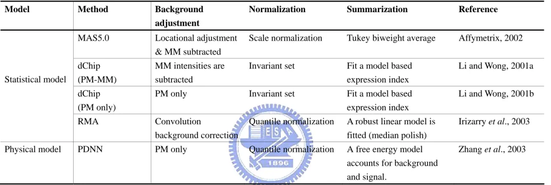
Table 1. Summary of the four preprocessing methods used ……… 49

Table 2. Summary of the three spike-in datasets used ………. 49

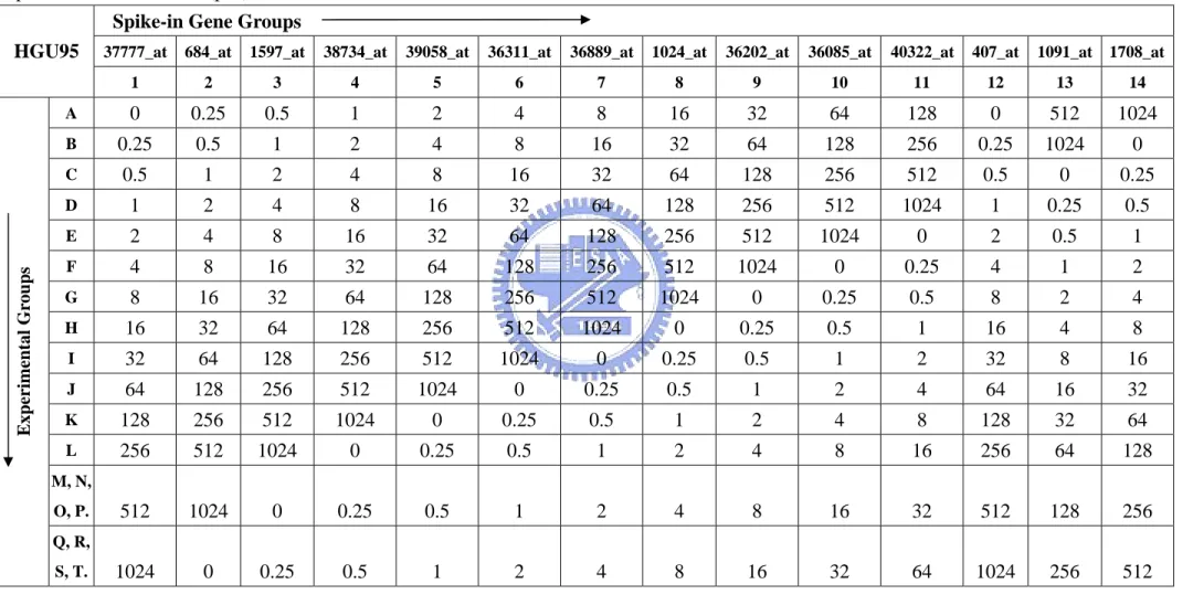
Table 3. Affymetrix human genome U95 dataset contains 14 spike-in gene groups in

each of 14 experimental groups. This table shows the spiked-in concentrations (pM) ……….…………..………….….. 50

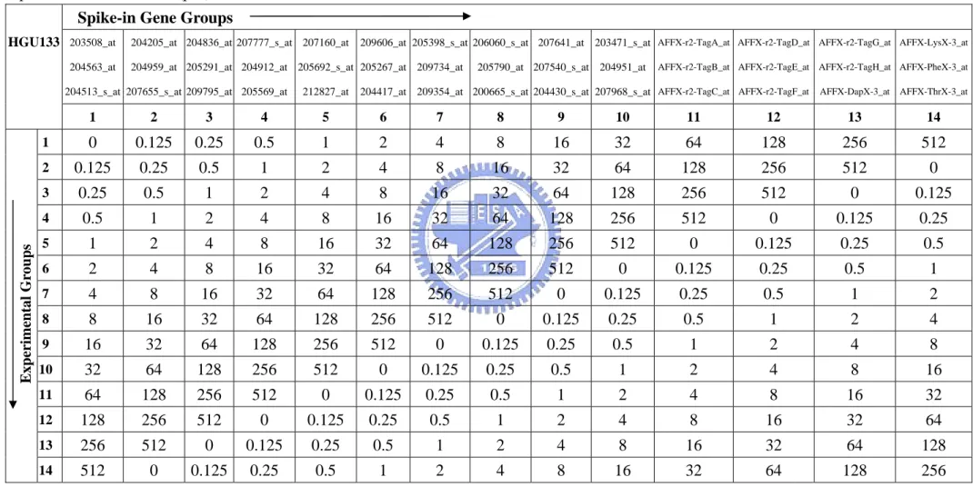
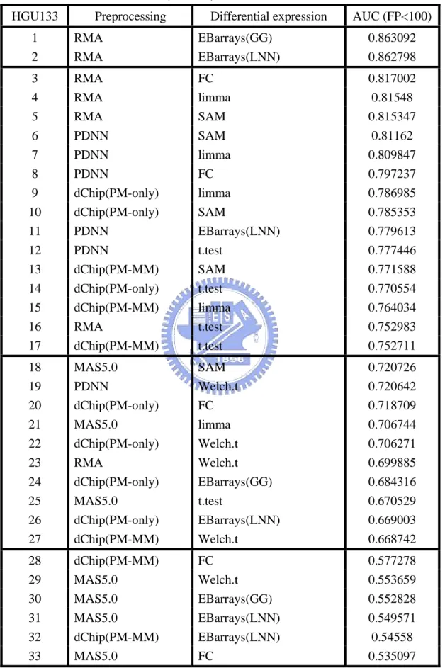
Table 4. Affymetrix human genome U133 dataset contains 14 spike-in gene groups in

each of 14 experimental groups. This table shows the spiked-in concentrations (pM) ……….…....………. 51

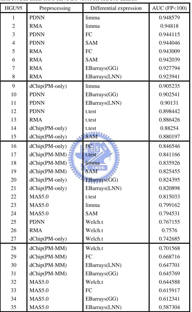
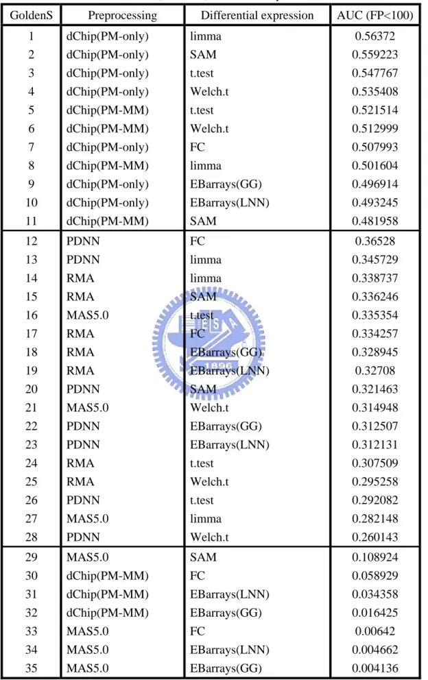
Table 5. Area under ROC curve (FP<100) for HGU95 dataset ……….…. 52 Table 6. Area under ROC curve (FP<100) for HGU133 dataset ……….... 53 Table 7. Area under ROC curve (FPR<0.1) for Golden Spike dataset ….. 54

List of Figures

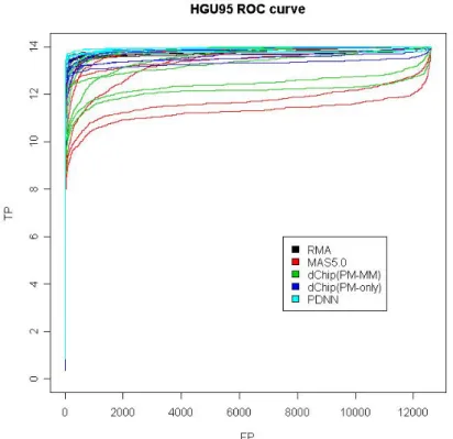
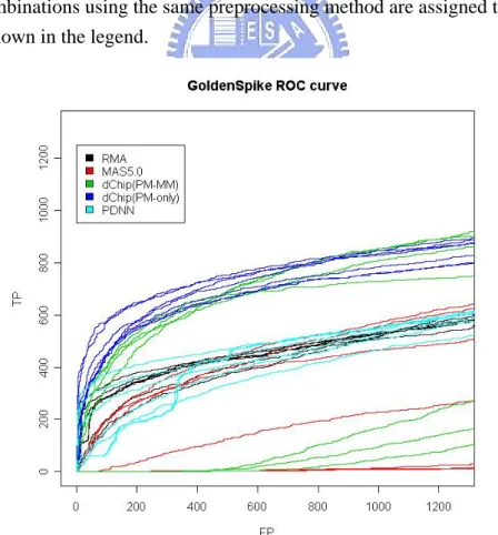
Figure 1-1. ROC curves for all combinations using HGU95 dataset. Combinations

using the same preprocessing method are assigned to the same color. ... 55

Figure 1-2. ROC curves for all combinations using HGU95 dataset but FP<100. 55

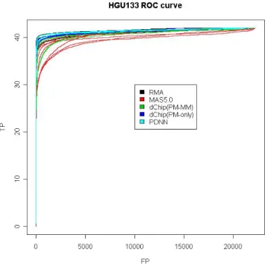
Figure 1-3. ROC curves for all combinations using HGU133 dataset. ………... 56 Figure 1-4. ROC curves for all combinations using HGU133 dataset but FP<100. 56

Figure 1-5. ROC curves for all combinations using Golden Spike dataset. ....… 57 Figure 1-6. ROC curves for all combinations using Golden Spike dataset but false

positive rate<0.1. …………...….……….……. 57

Figure 2-1. For HGU95 dataset, ROC curves of all combinations are divided by

preprocessing method. ……….……….… 58

Figure 2-2. For HGU133 dataset, ROC curves of all combinations are divided by

preprocessing method. ……….……….… 58

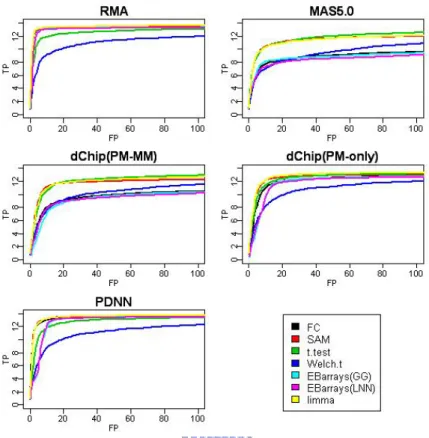
Figure 2-3. For Golden Spike dataset, ROC curves of all combinations are divided by

preprocessing method. ……….………. 59

Figure 3-1. ROC curves for all combinations using HGU95 dataset. Combinations

using the same differential expression method are assigned to the same

color. ……….……… 59

Figure 3-2. ROC curves for all combinations using HGU133 dataset. ………... 60 Figure 3-3. ROC curves for all combinations using Golden Spike dataset. …… 60 Figure 4. Overlap rate of two differentially expressed gene lists generated using

different combinations. ……….……….... 61

Figure 5-1. Overlap rate of two differentially expressed gene lists generated using

Figure 5-2. Overlap rate of two differentially expressed gene lists generated using

different combinations for L_AA treatment/control. ……….…..…………. 62

Figure 5-3. Overlap rate of two differentially expressed gene lists generated using

different combinations for L_CFY treatment/control. ……….……….…… 63

Figure 5-4. Overlap rate of two differentially expressed gene lists generated using

different combinations for L_RDL treatment/control. ……….….…… 63

Figure 6. Overlap rate of two differentially expressed gene lists generated using

different combinations with EBarrays as differential expression method. ... 64

Figure 7. Overlap rate of two differentially expressed gene lists generated using

different combinations. Combinations using the same differential expression method are assigned to the same color. ……….…………...……… 65

Figure 8. Overlap rate of two differentially expressed gene lists generated using nine

different combinations. ……..……….……….. 66

Figure 9-1. Average overlap rate of two differentially expressed gene lists generated

using different combinations. Combinations using the same preprocessing method are assigned to the same color. ……….………... 67

Figure 9-2. Average overlap rate of two differentially expressed gene lists generated

using different combinations. Combinations using the same differential

1 Introduction

Microarray is a device designed to simultaneously measure the expression levels of many thousands of genes in a particular tissue or cell type. It is widely used in many areas of biomedical research especially Affymetrix GeneChip platform. Millions of probes with length of 25 nucleotides are designed on an Affymetrix array. Two categories of probes are designed: “perfect match (PM)” probe perfectly matches its target sequence and “mismatch (MM)” probe is created by changing the middle (13th) base of its paired perfect match probe sequence. The purpose of designing MM probe is to detect the nonspecific binding because its perfect match partner may be hybridize to nonspecific sequences. A paired PM and MM is called a “probe pair” and each gene will be represented by 11-20 probe pairs typically. Owing to this distinctive design, preprocessing Affymetrix expression arrays usually involves three main steps. That are background adjustment, normalization, and summarization. Nowadays, a large number of preprocessing methods have been developed to estimate expression levels of genes.

Another fundamental goal of a microarray experiment is to identify those genes that are differentially expressed within different samples. For example, a disease may be caused by large expression of particular genes resulting in variation between diseased and normal tissues. The method used to detect the genes expressed differentially between different samples is called differential expression method. Various preprocessing and differential expression methods have been proposed, and their developers using different datasets and criteria claimed there are some features superior to other methods. In this thesis, we use the common datasets to evaluate combinations of the most popular preprocessing and differential expression methods in terms of validity and reliability. We try to help users of Affymetrix to select the best

method for their own microarray data.

Here we consider four commonly used preprocessing methods, Microarray Suite software Version 5.0 (MAS 5.0: Affymetrix, 2002), DNA-Chip Analyzer (dChip: Li and Wong, 2001a and 2001b), Robust Multi-array Analysis (RMA: Irizarry et al., 2003a) and Position-Dependent Nearest-Neighbor (PDNN: Zhang et al., 2003), and five popular differential expression methods, Fold change(FC), two sample t-test, Significance Analysis of Microarrays (SAM: Tusher, Tibshirani and Chu, 2001), Paramettric Empirical Bayes methods (EBarrays: Newton et al., 2001, Kendziorski et

al., 2003, and Newton and Kendziorski, 2003), and Linear Models and Empirical

Bayes methods (limma: Smyth, 2004). Four datasets in total are used. Three are spike-in datasets used to assess the validity: two from Affymetrix Latin square datasets and one from the Golden Spike Project. ROC curves are used for the evaluation. To evaluate the reliability, we use another dataset from MicroArray Quality Control (MAQC) project, which was generated using samples hybridized to Affymetrix platform at two different test sites. Overlap rates between two test sites are compared.

2 Literature

Review

2.1 Background of microarray

Microarray is a device designed to simultaneously measure the expression levels of many thousands of genes in a particular tissue or cell type. It is widely used in many areas of biomedical research. Microarray technology makes use of the sequence resources created by the genome projects and other sequencing efforts to detect which genes are expressed in a particular cell type of an organism. Many different microarray technologies have been developed, and can be classified into three main categories: cDNA array (highly variable in length), short oligonucleotide array (25-30 base) and long oligonucleotide array (50-80 base). The high-density oligonucleotide array produced by Affymetrix is one kind of the short oligonucleotide array. Affymetrix GeneChip arrays have become a widely used microarray platform and numerous of methods have been proposed for analyzing this type of microarray data. This thesis focuses on the analysis of data from Affymetrix GeneChip expression arrays.

2.2 Affymetrix GeneChip array

Affymetrix GeneChip array are high throughput assays for measuring the expression levels of many thousands of gene transcripts simultaneously in a particular tissue or cell type. The technology takes advantage of hybridization properties of nucleic acid. To measure how much quantity of specific nucleic acid transcripts of interest present in the sample, complementary molecules are used to attach to a solid surface. The specific nucleic acid transcripts of interest presented in the sample are referred as “target”, and the complementary molecules attached to a solid surface are referred as “probe”. Millions of probes with a usually length of 25 nucleotides are

produced on an Affymetrix array. Two categories of probes are designed, “perfect match (PM)” probe perfectly matches its target sequence, and “mismatch (MM)” probe is created by changing the middle (13th) base of its paired perfect match probe sequence. The purpose of designing MM probe is to detect the nonspecific binding because its perfect match partner may be hybridize to nonspecific sequences. A paired PM and MM are called a “probe pair”, and a gene represented by multiple probe pairs is called a “probeset”. Typically, each gene will be represented by 11-20 probe pairs. For more comprehensible, we show these in following graph.

After RNA samples were prepared, labeled and hybridized to an array with millions of probes, the array is scanned and pixel intensity values are calculated using peculiar instruments by Affymetrix. According to these values, intensity values for each probe, called probe-level intensities, are computed and stored in a CEL file. The next step is to find a way to combine the 11-20 probe pair intensities together to a summary value for a given gene. The summary value for a given gene is defined as a measure of expression that represents the amount of the corresponding mRNA species. However, due to many systematical biases from different sources in miroarray experiments, data preprocessing becomes more necessary and important. The goal of data preprocessing is to obtain a corrected intensity value that represents the abundance of mRNA, instead of an uncertain brightness biased by other sources. Preprocessing Affymetrix expression arrays usually involves three main steps:

background adjustment, normalization, and summarization, that is, low-level analysis of Affymetrix microarray. Details for preprocessing methods are described later.

Another fundamental goal of a microarray experiment is to identify those genes that are differentially expressed within different samples. For example, a disease may be caused by large expression of a particular gene or genes resulting in variation between diseased and normal tissues. Numerous of differential expression methods are proposed to detect those differentially expressed genes between diseased and normal tissues. Throughout this thesis, we attempt to compare those combinations of the most commonly used preprocessing methods and differential expressed methods.

2.3 Overview of preprocessing method

Here we interpret the three main steps of data preprocessing briefly before mentioning these preprocessing methods used to compare.

2.3.1 Background adjustment

Because partial measured probe intensities maybe caused by non-specific hybridization or the noise in the optical detection system, background adjustment is essential to rid of these intensities not exactly expressed from genes. Observed probe intensities need to be adjusted to give the accurate expression levels of specific hybridization (Huber et al., 2005). Some methods make use of MM probes to adjust, but some are not.

2.3.2 Normalization

During the process of carrying out the microarray experiment involving multiple arrays, there are many obscuring sources of variation involved, such as physical problems with the arrays, laboratory conditions, hybridization reactions, labeling, and scanner difference. In order to compare measurements from different arrays, implying different tissue, some proper normalization is necessary.

2.3.3 Summarization

Due to Affymetrix platform designing multiple probes to represent a gene, summarization is needed to combine these probe intensities to a single value. For each gene, the background adjusted and normalized intensities are used to be summarized into one measurement that estimates the expression level.

2.4 Four preprocessing methods used Notations: ) ( : , .... , 1 : ,...., 1 ) ( : ,...., 1 gene set probe the ng representi G g gene the in pair probe the ng representi J j sample array different the ng representi I i = = = MAS 5.0

MAS 5.0 (Microarray Suite software, Version 5.0) is offered by Affymetrix (Affymetrix, 2002). The gene expression level is calculated from the combined, background-adjusted, PM and MM values of the probe set. At the beginning, both PM and MM probe intensities must be preprocessed for background adjustment.

To do the background adjustment, the array is divided into K rectangular zones (default K = 16). The probes are ranked and the lowest 2% is chosen as the background

k

Z

b for that zone. Then each probe intensity is adjusted based on a

weighted average of each of the background values, b(x,y).

k Z K k k K k k b y x w y x w y x b

∑

∑

= = = 1 1 ) , ( ) , ( 1 ) , ( .

The weights for zone k, w_k(x,y), are dependent on distance from the probe location (x,y) to each of the zone centers. In particular, the weight is defined as:

smooth y x d y x w k k + = ) , ( 1 ) , ( ₂ ,

of zone k. The default value of smooth is 100, which is added to d_k2(x,y) to ensure that the value will never be zero. The calculated background, b(x,y) 1, establishes a “floor” to be subtracted from each raw probe intensity. There are some rules for avoiding leading to the negative intensity.

After each probe intensity is preprocessed for background adjustment, an ideal mismatch value is calculated and subtracted to adjust the PM intensity. Originally, the suggested purpose of the MM probes was that they could be used to adjust the PM probes for non-specific binding. The naïve approach is subtracting the intensity of MM probe from the intensity of the corresponding PM probe. However, this becomes problematic because the MM value is sometimes larger than the PM value. To avoid taking the negative expression value, Affymetrix introduced the concept of an Ideal

Mismatch (IM), a quantity derived from the MM value that is never bigger than its

corresponding PM value. IM is defined as a quantity equal to MM whenMM < PM, but adjusted to be less than PM whenMM ≥PM . This is done by computing thespecificbackground,SB_g, for each probe set g. If the g=1,…,G is the probe set and j=1,….,J is the probe pair, then the SB_g is defined as:

(

)

{

PM MM j J

}

Biweight Tukey

SB_g = log_{2 jg} −log₂( _jg): =1,…, ,

and theIM_jgfor probe pair j in probe set g is defined as:

⎪ ⎪ ⎪ ⎪ ⎪ ⎪ ⎩ ⎪⎪ ⎪ ⎪ ⎪ ⎪ ⎨ ⎧ ≤ ≥ > ≥ < = ⎟ ⎟ ⎟ ⎟ ⎟ ⎠ ⎞ ⎜ ⎜ ⎜ ⎜ ⎜ ⎝ ⎛ ⎟⎟ ⎠ ⎞ ⎜⎜ ⎝ ⎛ − + τ τ τ ττ contrast SB and PM MM PM contrast SB and PM MM PM PM MM MM IM g jg jg scale SB contrast contrast jg g jg jg SBg jg jg jg jg jg g , 2 , 2 , 1

where contrastτ(with a default value of 0.03) and scale (with a default value of τ

10) are tuning constants. The adjusted PM intensity is obtained by subtracting the corresponding IM from the observed PM intensity. Then, MAS 5.0 use a one-step Tukey Biweight to combine the probe intensities in log scale.

(

)

{

jg jg

}

g theanti of TukeyBiweight PM IM

signal = log log₂ − .

Finally, signal is scaled using a trimmed mean. They defined a scaling factor sf and a normalization factor nf in their algorithm.

) 98 . 0 , 02 . 0 , (signal TrimMean Sc sf = ,

where Sc is the target signal (default Sc=500). MAS 5.0 offers two analysis for user to choose, that are absolute analysis and comparison analysis. According to which analysis you want to perform, nf has different definition.

⎪⎩ ⎪ ⎨ ⎧ = analysis comparison for SPVe TrimMean SPVb TrimMean analysis absolute for nf , ) 98 . 0 , 02 . 0 , ( ) 98 . 0 , 02 . 0 , ( , 1

where SPVb is the baseline array signal, and SPVe is the experiment array signal. More details are described in the Statistical Algorithms Description Document (Affymetrix, 2002). The reported value of MAS5.0 of probe set g is:

g signal sf nf i e portedValu ( )= × × Re . dChip

dChip (DNA-Chip Analyzer) is also a popular software for Affymetrix platform probe-level and high-level analysis of gene expression microarrays (Li and Wong, 2001a) and SNP microarrays. This software can be downloaded from the website

http://biosun1.harvard.edu/complab/dchip/ . dChip can be used to fit the Model Based Expression Index (MBEI) (Li and Wong, 2001a) , and obtain what we refer to as the dChip expression measure. Li and Wong reported that variation of a specific probe across multiple arrays (the between-array variance) is in general smaller than the

variance across probes within a probe set (the within-probe set variance) (Li and Wong, 2001a). To account for this strong probe affinity effect, they proposed a multiplicative model, for any given gene:

ε φ α θ ν ε φ θ α θ ν ε α θ ν + + + = + + + = + + = ) ( _{j j} i j j i j i j ij j i j ij PM MM (1)

Here PM and _ij MM denote the PM and MM intensity values from the i-th array _ij

and the j-th probe pair for this gene. θ_i denotes the expression index for this gene in the i-th array. Here multiple arrays are available for analysis. Assume that the intensity value of a probe will increase linearly as θ_i increases, but different increasing rate for different probes. And within the same probe pair, the PM will _ij

increase at a higher rate than theMM . _ij α_j and φ_j represent the increasing rate of the MM probe and the additional increasing rate in the corresponding _ij PM probe _ij

respectively. The increasing rates are assumed to be nonnegative.ν_j is the baseline response of the j-th probe pair due to nonspecific hybridization, and ε are assumed to be independent normally distributed errors.

The model for individual probe responses implies an even simpler model for the PM–MM differences: ) 2 ( . ,..., 1 , ,..., 1 ,i I j J MM PM_ij − _ij =θ_iφ_j +ε_ij = =

The model above is called PM-MM difference model ( Li and Wong, 2001a).

Li and Wong discovered that because of doubting the efficiency of using MM probes, some investigators design custom arrays using PM probes exclusively. Thus, they proposed another model later to estimating gene expression levels, called PM-only model ( Li and Wong, 2001b). The PM-only model focus only on PM probes, using the description of PM in model (1). The PM-only model is as follows:

) 3 ( . ' ε φ θ ν ε φ θ α θ ν + + + = + + = _{j i j i j j i j} ij PM

Notations in the PM-only model represent the same meaning as well as PM-MM difference model, except that φ merges the two increasing rates 'j αj and φj.

No matter what model above is referred, Li and Wong’s measure is defined as the maximum likelihood estimates of the expression index θ_iand outlier probe intensities are removed as part of the estimation procedure. Before computing model-based expression levels, dChip use the “Invariant Set” normalization method to normalize arrays at PM and MM probe levels for PM-MM difference model or PM probe levels for PM-only model. Using a baseline array, arrays are normalized by selecting invariant sets of probes then using them to fit a non-linear relationship between the "treatment" and "baseline" arrays. A set of probe is said to be invariant if ordering of probe in one chip is the same in other set. By default, an array with median overall intensity is chosen and all other arrays are normalized to it.

In order to summarize the probe intensities, dChip performs the “Invariant Set” normalization method, then fit the normalized probe intensities to the alternative model for any given gene. Maximum likelihood estimates of the expression indexθ_iis the expression measure for this gene in array i.

RMA

RMA (Irizarry et al., 2003a), Robust Multi-array Analysis, is an expression measure consisting of three particular preprocessing steps: convolution background correction, quantile normalization, and a summarization based on a multi-array model fit robustly using the median polish algorithm. Many preprocessing methods, such as MAS 5.0 and dChip, calculating their measures rely on the difference PM-MM with the intention of correcting for non-specific binding. However, the exploratory analysis presented in Irizarry et al. (2003a) suggests that the MM probe may be a mixture

probe for which detects not only non-specific binding and background noise but also the transcript signal just like the PM probe. Thus, subtracting the MM intensity from the PM intensity as a way of correcting for non-specific binding and background noise is not always appropriate. These RMA authors proposed a procedure ignoring the MM intensities and using only the PM intensities.

The RMA convolution background correction method is motivated by looking at the distribution of probe intensities. The model observed PM as the sum of a background intensity bg caused by optical and nonspecific binding, and a signal _ijg

intensity s . _ijg G g J j I i s bg

PM_ijg = _ijg + _ijg , =1,…, , =1,…, , =1,…,

with i representing the different array, j representing the probe pair, and g representing the different probe set. Under the model above, the background corrected probe intensities will be given by B(PM_ijg), where B(PM_ijg)≡E(s_ijg |PM_ijg). To obtain a computationally feasible B(⋅) we consider the closed-form transformation obtained when assuming that s is distributed exponential and _ijg bg is distributed normal, _ijg

and the results obtained using B(⋅) work well in practice (Irizarry et al., 2003a). Next, perform the quantile normalization, which is to make the distribution of probe intensities for each array the same (Bolstad et al., 2003). In order to summarize the probe intensities, RMA introduced a log scale linear additive model. The model is:

ij j i ij e a PM T( )= + +ε ,

where PM_ijg represents the PM intensity of array i=1,…,I and probe pair j=1,…,J, for any given probe set g. T

( )

⋅ represents the transformation that background corrects, normalizes, and logs the PM intensities, e represents the log2 scale _i

expression value found on arrays i, a represents the log scale affinity effects for _j

probes j , and ε_ij represents error (Irizarry et al., 2003b). To protect against outlier probes, they use a robust procedure, such as median polish, to estimate model parameters (Irizarry et al., 2003a). The estimate of e as the log scale measure of _i

expression refers to as robust multi-array average (RMA).

PDNN

Zhang et al. (2003) propose a simply free energy model over the probe signals

that enables to estimate the gene expression levels, called “position-dependent nearest–neighbor (PDNN) model”, for the formation of RNA-DNA duplexes on Affymetrix microarray. Different from most methods focused on statistical models, it is a physical model taking into account the sequence of nearest-neighbors (adjacent two bases) and the position of these nucleotide pairs. It has been suggest that the effect of nearest-neighbor nucleotide pairs is the most important factor in determining RNA/DNA duplex stability. Their model also describes binding interactions complicated by many factors such as steric hindrance on the chip surface, probe-probe interaction and RNA secondary structure formation.

The model is based on the nearest-neighbor model (Sugimoto et al., 1995) with two modifications: (1) a positional weight factor is added to reflect the different contributions from different part of the probe; (2) two different types of binding on the probes are considered. The two types of binding are gene-specific binding (GSB), representing the formation of DNA-RNA duplexes with exact complementary sequences, and non-specific binding (NSB), representing the formation with many mismatches between the probe and the attached RNA molecule. Notice that PDNN assumes that the majority of probes are designed specifically for their target, and only PM probes are used for GSB and NSB estimation. PDNN model divides signal of a

probe into three components, GSB, NSB and uniform background B, as follows: B e N e N I jg jg E E g jg + + + + = * 1 1 ˆ * _,

where Iˆ is denoted as the expected intensity of the j-th probe in a probe set _jg

targeted to detect gene g, N as the true expression level for gene g, and g *

N as the

population of RNA molecules that contributes to NSB. E is defined as the free _jg

energy for formation of the specific RNA-DNA duplex with the targeted gene, and *

jg

E is the average free energy for NSB, that is, formation of duplexes with many different genes. E and _jg E*_jg are computed as weighted sums of stacking energies with the sequence of a probe is given as

(

b₁,b₂,...,b₂₅

)

.

(

)

(

)

∑

∑

= + = + = = 24 1 1 * * * 24 1 1 , , k k k k jg k k k k jg b b E b b E ε ω ε ω

with ω_k and ω representing weight factors that depend on the position along the _k* probe from the 5’ end to the 3’ end, and ε

(

b_k,b_k+1

)

is defined the same as the stacking energy used in the nearest-neighbor model (Sugimoto et al., 1995). Both of GSB and NSB are involving 16 stacking energy parameters and 24 weight factors.

The unknown parameters are obtained by minimizing the fitness function F to optimize the match between the expected probe intensity Iˆ and the observed probe _jg

intensityI . _jg

(

)

∑

− = M I I F jg jg 2 ln ˆ ln ,

where M is the total number of probes on an array. A Monte Carlo simulation procedure is used to minimize the fitness function F. When the parameters are given,

the gene expression level N can be calculated and are scaled to an average of 500 _g

on an array.

For more comprehensible, we give a summary table for the four preprocessing methods above in Table 1.

2.5 Five differential expression methods used Fold-change

Fold-change is the most commonly used method of detecting differentially expressed gene between two compared condition samples. It is often the first method used in microarray analysis. For any given gene, fold-change is calculated by the probeset intensity ratio of two compared condition samples. If there are replicates, we usually average across the samples for each condition in advance. Then the ratio of these averaged values is referred as fold-change. Larger fold-change leads the gene to be more likely differentially expressed gene. Biologist favors fold-change equal to 2 as the threshold of differential expression.

Two sample t-test

The simplest statistic method for comparing means between two groups is two sample t-test. It is widely applied in microarray analysis when detecting the differentially expressed genes between two compared condition samples. For any given gene, assume that the measurements of the first condition sample arise independently and identically from normal distribution with mean μ and variance ₁

2 1

σ , and the measurements of the second condition sample arise independently and

identically from normal distribution with mean μ₂ and variance σ₂2 . When carrying out a two sample t-test, the variances of the two samples may be assumed to

be equal or unequal. The approach of unequal variance assumption is also called Welch’s t-test. For any given gene g, suppose that the number of samples in condition1 and in condition2 are M and N respectively. Here we describe the two tests briefly.

Two sample t-test for equal variance:

. 2 ) ( ) ( , ~ 1 1 : : : H ) , ( ~ ,..., : 2 ) , ( ~ ,...., : 1 1 2 1 2 2 2 2 1 1 2 1 0 2 2 1 2 1 1 − + − + − = + − ≠ =

∑

∑

= = − + N M Y Y X X S where T S N M Y X statistic test H versus N Y Y condition N X X condition N i i M i i p N M p gN g gM g μ μ μ μ σ μ σ μ

Two sample t-test for unequal variance (Welch’s t-test):

. ) 1 ( ) 1 ( ) ( ) ( 1 1 , ) ( 1 1 ), ( ~ ) ( : : : H ) , ( ~ ,..., : 2 ) , ( ~ ,...., : 1 2 4 2 4 2 2 2 1 2 2 1 2 2 2 2 2 1 1 2 1 0 2 2 2 1 2 1 1 1 − + − + = − − = − − = + − ≠ =

∑

∑

= = N N S M M S N S M S and Y Y N S X X M S where ely approximat T N S M S Y X statistic test H versus N Y Y condition N X X condition Y X Y X N i i Y M i i X v Y X gN g gM g ν μ μ μ μ σ μ σ μ

After performing the test and the conclusion leads to rejectH , we consider that this ₀

gene is a differentially expressed gene.

SAM (Significance Analysis of Microarrays)

SAM is a method for identifying genes on a microarray with statistically significant changes in expression. It was proposed by Tusher, Tibshirani and Chu

(2001). The method is based on a modified version of the standard t-statistic. Standard t-statistic method is popular but having the problem of multiple testing. That is, when thousands of hypotheses are tested simultaneously in microarray experiment, it would increase chance of false positives. For example, if we have 10000 genes in our microarray experiment and all of them are non-differentially expression. Choosing significance level α =0.01, we would expect that there are 10000×0.01=100 genes called significant (having p− value<0.01). Even if we choose a small

01 . 0 =

α to evaluate small numbers of genes, we still get 100 genes called significant because of multiple testing. This problem led them to develop a statistical method adapted specifically for microarrays, Significance Analysis of Microarrays (SAM). For each gene g, the “relative difference” d in gene expression is: _g

0 s s r d g g g = ₊ .

Here r is a score, _g s is a standard deviation, and _g s is an exchangeability factor ₀

(Chu et al.). SAM software can be adapted for many types of experimental data, such as a simple unpaired two-group data, multiple-group data, paired data, censored survival data, …, etc. For each type of experimental data, SAM defines different

g g and s

r in a different way (Chu et al.). We now focus only on the experiment of two groups. In this case, r_g and s_g have the following definition:

, 2 ) ( ) ( ) 1 1 ( 2 1 2 2 2 1 2 1 2 1 1 2 − + − + − × + = − =

∑

∑

∈ ∈ n n x x x x n n s x x r group i g gi group i g gi g g g g

where x and _g1 x are defined as the average levels of expression for gene g in _g2

sample i. Group 1 and 2 have n₁ and n₂ genes, respectively. Comparing with standard two sample t-statistic for equal variance, the test statistic is the same as

g g

s r

. It is a problem with low expression levels genes. That is, variance in g g

s r

can

be high because of small values ofs . But in order to compare values of _g d across _g

all genes, the distribution of d should be independent of the gene expression level. _g

Thus, SAM adds s in the denominator to ensure that the variance of ₀ d is _g

independent of gene expression level. The value for s is chosen to minimize the ₀

coefficient of variation. Rank all genes from small to large by d and denote new _g

arrangements as d_{( g)}. In other words, d_{( g)} is the g-th smallest relative difference. To identify differentially expressed genes, a scatter plot of the observed relative difference d_{( g)} vs. the expected relative difference d_{( g)}* is used. The definition of the expected relative difference d_{( g)}* is as follows. Take B sets of permutations of the samples, and re-calculate a new “relative difference” d_g*b for each permutation b. Obtain the corresponding order statistics d_(g)*b by ranking d_g*b from small to large for each permutation b. For each permutation b, estimate the expected order statistics

by

∑

= = B b b g g d B d 1 * ) ( * ) ( 1 .

In the scatter plot mentioned above, each points represents a specify gene. Choosing an adequate value as threshold Δ , the genes apart from the d_(g) =d₍*_g)

line by a distance greater than the threshold Δ are regarded as differentially expressed genes. Using the samr package in R, the differentially expressed genes can be identified by giving a threshold Δ .

EBarrays

EBarrays package is implemented in the Bioconductor which is an open source and open development software project for the analysis and comprehension of genomic data (http://www.bioconductor.org/). EBarrays is an empirical Bayes analysis for identifying differentially expressed genes between two or among more than two conditions. The models attempt to describe the probability distribution of a set of expression measurements taken on a gene g, and select differentially expressed genes by posterior probability of expression pattern, which is computed for each gene and for each pattern. For more details on the methodology, see Newton et al. (2001), Kendziorski et al. (2003) and Newton and Kendziorski (2003).

Measurements are considered as arising from an observation distribution )

|

( _g

obs

f ⋅ μ , where μ_g is a gene-specific mean value. The number of mean expression patterns possible depends on the number of conditions in a microarray experiment. For example, with a typical two conditions experiment, there are two possible patterns of expression - equivalent expression and differential expression between the two conditions. With three conditions, there are five possible patterns among the means. One pattern is equivalent expression across all conditions, and one pattern is distinct expression in each condition. Notice that different conditions may be sharing a common mean expression level, thus there are three patterns for altered expression in just one condition.

Suppose in the general case of I arrays including N conditions, there are m+1 possible distinct patterns. For gene g, ( ,..., )

~ 1 ~ ~ g g gN d d

d

= denotes the data vector where the measurements among the same condition cluster together. For any pattern k, the expression measurements sharing the common mean expression level group into the same subset. Thus, the N conditions are partitioned into r(k) mutually exclusive

and exhaustive subsets

{

S_t,k;t=1,2,...,r(k)

}

. Assume that measurements sharing a common mean expression level μ_g arise independently and identically from an observation component f_obs(⋅| μ_g) , and μ_g arise from some genomewide distribution )π(μ_g . Two parametric forms, Gamma-Gamma and Lognormal-Normal models, are considered later. Denote ( )

,

, ~gS_tk

d

f as the pdf for the data indexed by

subset S_t,k. g g S s g s g obs S g f d d d f k t k t μ μ π μ ) ( ) | ( ) ( , , ` , , ~

∫ ∏

⎟ ⎟ ⎠ ⎞ ⎜ ⎜ ⎝ ⎛ = ∈

The pattern specific predictive density for pattern k is given by

∏

= = ( ) 1 ~ , ~ ) ( ) ( , k r t gS g k k t d f d f

where k=0 denotes the null hypothesis which is equivalent expression among all conditions. For each gene, discrete mixing parameters p , k=1,…,m+1 are _k

introduced to denote the unknown probabilities of expression pattern k, and describe the marginal distribution of the data by a mixture of the form

∑

= m k g k kf d p 0 ~ ) (

The posterior probability of expression pattern k is then ) ( ) | ( ~ ~g pkfk dg d k P ∝

and the posterior odds in favor of pattern k is

) ( 1 ) ( 1 ~ ~ , g k g k k k k g d f d f p p odds − − =

The authors consider two particular distributional forms of the general mixture model described above. The way to specify the model is determined by the choice of

observation component f_obs(⋅| μ_g) and mean component π(μ_g). Gamma-Gamma model (GG model):

Assume that the observation component f_obs(⋅| μ_g) is a gamma distribution having shape parameter α >0 and scale parameter

g μ

α

λ = for measurements

greater than zero, and assume a constant coefficient of variation

α

1

in this distribution. They take the mean component π(μ_g) to be an inverse gamma, i.e. the quantity

g

g _μ

α

λ = has a gamma distribution with shape parameter α₀ and scale parameterν . Thus three parameters are involved in GG model, θ =(α,α₀,ν).

Lognormal-Normal model (LNN model):

Assume that the observation component f_obs(⋅| μ_g) is a log-normal distribution with mean μg and variance

2

σ , and assume a constant coefficient of variation on

the raw scale in this distribution. A conjugate prior for the μ_g is normal with mean

0

μ and variance τ02 . Thus three parameters are involved in LNN model,

) , , ( 0 2 0 σ τ μ θ = .

The optimal procedure to classify genes into certain expression pattern is according to the state favored by the posterior probabilities. In general, in a typical two conditions experiment, genes with posterior probability of differential expression pattern greater than 0.5 are identified as the most likely differentially expressed genes (Kendziorski et al., 2007). For more details on the methodology, see Newton et al. (2001), Kendziorski et al. (2003) and Newton and Kendziorski (2003).

limma

analysis of data arising from single channel such as Affymetrix and long-oligos or two channel such as cDNA microarray experiments. The central idea is to fit a linear model to the expression data for each gene (Smyth, 2004). The linear model for gene g is: g g X y E ~ ~ ~ ) ( = α , where g y ~

contains the expression data for the gene g, ~

X is the design matrix, and

g ~

α is a vector of coefficients. This model is specified by the design matrix ~

X . If we

have a set of I microarrays in our experiment, the response vector of the linear model is y_gT =

(

y_g1,...,y_gI

)

for gene g. The responses will usually be log-intensities for single channel data or log-ratios for two-color data. Certain contrasts of the coefficients are assumed to be of biological interest and these are defined by

g T g C ~ ~ ~ α β = .

In general, we are interested in testing whether individual contrast values β_gj are equal to zero. For example, with a three conditions experiment, if we concern whether there are difference between condition 1 and 2 and between condition 2 and 3 respectively, we may set the design matrix X and the contrast matrix C as follows

⎥ ⎥ ⎥ ⎦ ⎤ ⎢ ⎢ ⎢ ⎣ ⎡ = ⎥ ⎥ ⎥ ⎥ ⎥ ⎥ ⎥ ⎥ ⎦ ⎤ ⎢ ⎢ ⎢ ⎢ ⎢ ⎢ ⎢ ⎢ ⎣ ⎡ = 1 0 1 -1 0 1 -1 0 0 1 0 0 0 1 0 0 1 0 0 0 1 0 0 1 C and X .

Then, test the hypotheses β_g1 =0 and β_g2 =0 individually.

The basic statistic used for hypothesis test with respect to a certain contrast βgj is the moderated t-statistic in which posterior residual standard deviations are used in

place of ordinary standard deviations. They use the empirical Bayes approach to shrink the estimated sample variances towards a common value, resulting in far more stable inference for small numbers of arrays. Additionally, they proposed an alternative statistic, called B-statistic which is log posterior odds that the gene is differentially expressed. The posterior odds are in terms of a moderated t-statistic. The B-statistic is monotonic increasing in the moderated t-statistic under some conditions. Even if these conditions do not hold, the two statistics will rank the genes in very similar order. To test hypotheses about all contrasts simultaneously, a moderated F-statistic which is appropriate quadratic forms of moderated t-statistic is used.

2.6 Datasets

Our purpose is to evaluate which combination of preprocessing and differential expression methods performs well. We attempt to evaluate both validity and reliability of these combinations. To properly compare the combinations in terms of validity, we request that the truth differentially expressed genes of the dataset must be known. One kind of microarray experiment is called “spike-in experiments”, that is, some gene fragments have been added at known concentrations. These genes are called spike-in genes. To evaluate the validity, we choose three spike-in datasets, human genome U95 dataset from Affymetrix, human genome U133 dataset from Affymetrix, and a wholly defined control spike-in dataset (Choe et al., 2005). To properly compare the method combinations in terms of reliability, we use a dataset which was generated using samples from rats and these samples are averagely distributed to different test sites (Guo et al., 2006). We use four datasets in total, and describe all briefly as follow.

Affymetrix human genome U95 dataset (HGU95)

The human data set with array type HG-U95A consist of a series of genes spiked-in at known concentrations and arrayed in a format analogous to cyclic Latin

Square format. But there is still a little different from cyclic Latin Square. They represent a subset of the data used to develop and validate the Affymetrix Microarray Suite (MAS) 5.0 algorithm.

A standard 14×14 cyclic Latin Square design must consist of 14 gene groups in 14 experimental groups. Each gene group contains only one spike-in gene, and each experimental group contains the same 14 spiked-in gene groups but spiked-in at different concentrations. For example, the concentration of the 14 gene groups in the first experimental group is 0, 0.25, 0.5, 1, 2, 4, 8, 16, 32, 64, 128, 256, 512, and 1024pM. Each subsequent experimental group rotates the spike-in concentrations by one group; i.e. experimental group 2 begins with 0.25pM and ends at 0pM, on up to experimental group 14, which begins with 1024pM and ends with 512pM. Except for the 14 spike-in genes, a common background cRNA have been added at all arrays.

The Affymetrix human genome U95 dataset contains 14 human genes in each of 14 experimental groups. Most groups contain 1 gene. Exceptions are group 1, which contains 2 genes, and group 12, which is empty. Specifically, transcript 407_at listed as present in group 12 is actually included in group 1 (together with 37777_at). For more comprehensible, we show the details in Table 3. The columns represent the 14 spiked-in gene groups and the rows represent the 14 experimental groups. The first row shows the gene name in each gene group.

Most experimental groups contain 3 replicates, except that the 3rd experimental group contain only 2 replicates and both the 13th and 14th experimental group contain 12 replicates. Replicates within each group result in a total of 59 arrays. This dataset is available at http://www.affymetrix.com/support/technical/sample_data/datasets.affx

Some researchers reported that there are 16 spike-in probesets in this dataset as opposed to the 14 originally described by Affymetrix (Cope et al., 2004). The two

pattern of gene group 12 missing from the Latin Square, agreed by three methods of calculating expression (RMA, MAS 5.0, dChip). Wolfinger and Chu (2002) identified this as well. They also claimed "546_at" should be considered with the same concentration as "36202_at" in gene group 9, since it has pattern the same as "36202_at", as shown by three methods. Wolfinger and Chu (2002) identified this as well. Due to the competitive preprocessing methods we choose are not merely the three methods, recognizing the two genes as spike-in genes maybe not advisable. For this reason, we recognize the 14 genes orginially described by Affymetrix as the entire spike-in genes.

Affymetrix human genome U133 dataset (HGU133)

This dataset with a particular array type HG-U133A_tag consist of more genes spiked-in at known concentrations and arrayed in a cyclic Latin Square format. The dataset is expected to be useful for the development and comparison of expression analysis methods. Distinct from the HGU95 dataset above, this data set includes many more spikes, and a smaller concentration spike (0.125pM).

This dataset consists of 14 spiked-in gene groups in 14 experimental groups. Distinct from the HGU95 dataset above, each gene group contains three spike-in genes. Thus there are 42 spike-in genes in total in this dataset. Each experimental group contains the same 42 spiked-in genes, but the genes in different gene group are spiked-in at different concentrations. For example, the concentration of the 14 gene groups in the first experimental group is 0, 0.125, 0.25, 0.5, 1, 2, 4, 8, 16, 32, 64, 128, 256, and 512pM. Each subsequent experimental group rotates the spike-in concentrations by one group; i.e. experimental group 2 begins with 0.125pM and ends at 0pM, on up to experimental group 14, which begins with 512pM and ends with 256pM. For more comprehensible, we show the details in Table 4.

The same as HGU95 dataset, all arrays have a common background cRNA except for the 42 spike-in genes. Each experimental group contains 3 replicates, and replicates within each group result in a total of 42 arrays. This dataset is available at

http://www.affymetrix.com/support/technical/sample_data/datasets.affx .

A wholly defined control spike-in dataset

Due to the vast numbers of genes interrogated in a microarray experiment, only a relatively small fraction of gene expression differences tend to be validated in any given study. Choe et al. (2005) generated a new control dataset for the purpose of

evaluating methods for identifying differentially expressed genes between two sets of triplicated hybridizations to Affymetrix GeneChips. The two sets are called spike-in samples and control samples, resulting in a total of 6 arrays. This dataset has three main features to facilitate the relative assessment of different analysis options. First, this experiment has 1331 spike-in genes spiked-in at known relative concentrations between the spike-in and control samples. The dataset has a larger fraction of gene expression differences than the general spike-in datasets. Second, this experiment used a defined background sample of 2535 genes presented at identical concentrations in both spike-in and control samples, rather than a biological RNA sample of unknown composition. Third, this dataset includes lower fold changes, beginning at only a 1.2-fold concentration difference to 4-fold concentration difference. This dataset is available at http://www.ccr.buffalo.edu/halfon/spike/index.html.

Here, we give a summary table for the three spike-in datasets in Table 2.

Rat dataset

The dataset we used is just a part of the complete dataset from a rat toxicogenomic study, which is one of the reference datasets of MAQC (MicroArray Quality Control) project

the MAQC project is to provide quality control tools to the microarray community in order to avoid procedural failures and to develop guidelines for microarray data analysis by providing the public with large reference datasets along with readily accessible reference RNA samples. The rat toxicogenomic dataset was generated using 36 RNA samples from rats treated with three chemicals (aristolochic acid, riddelliine and comfrey). In total there were six treatment/tissue groups: kidney from aristolochic acid–treated rats (K_AA), kidney from vehicle control (K_CTR), liver from aristolochic acid–treated rats (L_AA), liver from riddelliine- treated rats (L_RDL), liver from comfrey-treated rats (L_CFY) and liver from vehicle control (L_CTR). Within each treatment/tissue group there were six biological replicates. Aliquots of these samples were prepared and distributed to each of the test sites for gene expression profiling using microarrays from four different platforms (Affymetrix, Agilent, Applied Biosystems and GE Healthcare). There are two test sites using Affymetrix platform, and we adopt only the data from the two test sites. Each test site generated 36 arrays respectively. In this paper, when we refer to the Rat dataset, it denotes the 72 arrays in all which were generated from the two sites using Affymetrix platform. This dataset is available at

3 Materials and Methods

Our purpose is to evaluate which combinations of preprocessing and differential expression methods perform well. Specifically, we compare the combinations according to two main criteria, the validity and the reliability of the combinations. First, we select datasets having some particular properties in terms of different criteria and some interested preprocessing method is used on the datasets to summary the probe set measurements. Then, these measurements of genes are performed by some interested differential expression method, and the likely differentially expressed genes chosen by certain combination of preprocessing and differential expression method are listed. Based on the list of differentially expressed genes, we can evaluate the validity and the reliability of the combination. We divide the assessment of validity and reliability into two Sections 3.2 and 3.3 respectively in detail.

3.1 Implementation of methods selected

There are four preprocessing methods and five differential expression methods applied to each of the datasets we selected. Three statistical models, MAS 5.0, dChip and RMA, and one physical model, PDNN, are considered. The five differential expression methods are fold-change, two sample t-test, SAM, EBarrays and limma. A total of 35 combinations are resulted. We may regard each criterion of methods as “score” to express the level of significance. The higher the score, the more significant the result.

3.1.1 Four preprocessing methods used MAS 5.0

(Affymetrix, 2002). Each probe including PM and MM must be preprocessed for background adjustment according to its location on the array. To avoid obtaining a negative value when subtracting MM from PM, MAS 5.0 introduces the concept of an Ideal Mismatch (IM) derived from MM and never bigger than its PM. The expression level is defined as the anti-log of a robust average (Tukey biweight) of the value

(

)

{

log2 PMjg −IMjg

}

where PMjgand IMjg represent the PM and IM intensities for j-th probe pair of gene g. Finally, the expression level is scaled using a trimmed mean. We apply the absolute analysis of MAS 5.0 in R.

dChip ( including dChip(PM-MM) and dChip(PM-only))

Li and Wong (2001a) proposed a Model Based Expression Index model (MBEI) where multiple arrays are available to estimate the expression levels. For any given gene, the model is defined as follows:

ε φ α θ ν ε φ θ α θ ν ε α θ ν + + + = + + + = + + = ) ( _{j j} i j j i j i j ij j i j ij PM MM (1)

where PM and _ij MM denote the PM and MM intensity values from the i-th array _ij

and the j-th probe pair for this gene. θ_i denotes the expression index for this gene in the i-th array. α_j and φ_j represent the increasing rate of intensity value of the

ij

MM probe and the additional increasing rate in the corresponding PM probe _ij

respectively. ν_j is the baseline response of the j-th probe pair due to nonspecific hybridization, and ε are assumed to be independent normally distributed errors. Two methods based on the model above are developed: (1) subtracting MM from PM intensities (Li and Wong, 2001a) (2) using PM intensities only (Li and Wong, 2001b). Li and Wong’s measure is defined as the maximum likelihood estimates of the expression index θ_i and the estimation procedure includes rules for outlier removal.

“Invariant Set” normalization method is used to normalize arrays at PM and MM probe levels.

RMA

Irizarry et al. (2003a) developed a log scale linear additive model using only PM

probes, it is also known as RMA (Robust Multi-array Analysis). For any given gene, it is described as T(PM_ij)=e_i +a_j +ε_ij, where PM is the PM intensity of array i _ij

and probe pair j for this gene. T(⋅) represents the transformation that background corrects, normalizes by quantile normalization, and logs the PM intensities. The three terms on the right represent the log2 scale expression value for this gene of array i, the log scale affinity effects for probe j, and error respectively (Irizarry et al., 2003b). To

protect against outlier probes, a robust procedure such as median polish is used to estimate model parameters and the log scale measure of expression levele . _i

PDNN

Zhang et al. (2003) proposed a simply free energy model, called

“position-dependent nearest–neighbor (PDNN) model”. Different from most methods focused on statistical models such as the methods introduced above, it is a physical model taking into account the sequence of nearest-neighbors (adjacent two bases) and the position of these nucleotide pairs. In the PDNN model, the signal of a probe is divided into three components: gene-specific binding, non-specific binding, and uniform background. And the free energy of the two bindings of a probe can be expressed as a weighted sum of its stacking energies (Sugimoto et al., 1995), where the stacking energies depend on the sequence of nearest-neighbors and the weights depend on the position along the probe. Further technical details can be found in Zhang et al. (2003).

3.1.2 Five differential expression methods used Fold-change (FC)

Fold-change is the most commonly used method of detecting differentially expressed gene between two compared condition samples. For any given gene, fold-change is calculated by the probe set intensity ratio of two compared condition samples. If there are replicates, we usually average across the samples for each condition in advance. Then the ratio of these averaged values is referred as fold-change. Fold-change is employed as the score of significance.

Two sample t-test ( including t-test and Welch t-test)

The simplest statistical method for comparing means between two groups is two sample t-test. When carrying out a two sample t-test, the variances of the two samples may be assumed to be equal or unequal. The approach of unequal variance assumption is also called Welch’s t-test. We employ minus p-value as the score of significance.

SAM (Significance Analysis of Microarrays)

It was proposed by Tusher, Tibshirani and Chu (2001). The method is based on a modified version of the standard t-statistic to adjust the high variance probably caused by a low expression level. For each gene g, the “relative difference” d in gene _g

expression is defined as the form which adds an exchangeability factor to the denominator of the standard two sample t-statistic for equal variance. Exchangeability factor is added to ensure that the variance of d is independent of gene expression _g

level. Rank all genes by the observed relative difference d and denote the new _g

arrangements as d_{( g)}. B sets of permutations of the samples are taken to obtain the expected relative difference d_{( g)}* by a similar way (For more details, see Tusher et