非線性結構方程模式：以試題反應模式分析類別反應變項

非線性結構方程模式：以試題反應模式 分析類別反應變項

摘 要

人類學科裡的反應變項通常是二元或順序的，而不是等距。由於類別 的試題反應跟其所欲測量的潛在特質的關係不會是線性的，於是就發展了 試題反應理論來描述它們之間的非線性關係。另一種類別資料分析方法，試 圖建立潛在連續反應與所欲測量的潛在特質的線性關係，然後透過閾值模式 將潛在連續反應轉化為觀察的類別反應。當結構方程模式裡的測量模式中的 試題反應與潛在特質之間的關係是非線性時，就可稱為非線性結構模式。其

參數可用貝氏（WinBUGS軟體）或非貝氏（Mplus軟體）來估計。從模擬研

究裡，我們發現雖然這兩種軟體都可以很精確的估計參數，但當測驗短時，

WinBUGS 的估計效果比Mplus好。如果原始試題反應不可得的話，使用可 能值的作法可以有效估計內衍變項和外衍變項間的結構參數，但是最大概似 估計的作法嚴重低估結構參數，因為它完全沒有考慮測量誤差。兩個實證的 例子說明了非線性結構模式和可能值作法的意涵與應用。

關鍵詞：試題反應理論、潛在反應、非線性結構模式、貝氏統計、可能值 蘇啟明

國立中正大學心理學研究所博士候選人

王文中

香港教育學院心理研究學系講座教授

Abstract

Response variables in the human sciences are often binary or ordinal rather than interval. Because the relationship between categorical item responses and their underlying latent traits cannot be linear, item response theory (IRT) models have been developed to describe the nonlinear relationship between them. Another approach to categorical data is to establish linear relationship between latent continuous responses and their underlying latent traits and convert latent continuous responses to observed categorical item responses via threshold models. When the relationships between item responses and their underlying latent traits are nonlinear in the measurement part of structural equation modeling (SEM), the resulting SEM can be called nonlinear SEM (NSEM), to emphasize the nonlinear relationships between item responses and the underlying latent traits. Parameters in NSEM can be estimated using the Bayesian (WinBUGS) or non-Bayesian (Mplus) approaches. In a series of simulations, it was found that although both WinBUGS and Mplus can recover parameters in NSEM very well, WinBUGS slightly out-performs Mplus when tests are short. When original item responses are not accessible, the use of the plausible-value approach can recover the structural parameters for exogenous and endogenous variables as satisfactorily as WinBUGS and Mplus can when original responses are accessible.

However, the use of the maximum likelihood estimate approach underestimates the structural parameters substantially because the measurement error is ignored completely.

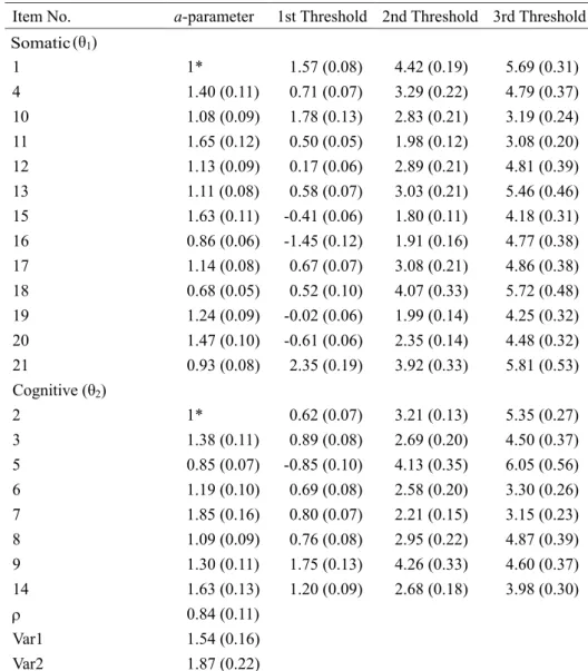
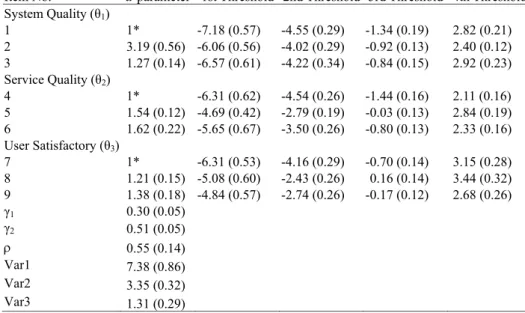
Depression and resource planning are two empirical examples that illustrate the implications and applications of NSEM and the plausible-value approach.

Keywords: item response theory, latent response, nonlinear structural equation modeling, Bayesian statistics, plausible value

Chi-Ming Su

Doctoral Candidate, Department of Philosophy, National Chung Cheng University, Chia-Yi, Taiwan

Wen-Chung Wang

Chair Professor, Department of Psychological Studies, The Hong Kong Institute of Education, Hong Kong

Nonlinear Structural Equation Models: An Item Response

Modeling Approach to Categorical Response Variables

Many attributes in the human sciences can be investigated only indirectly through observable indicators, because they are hypothetical constructs. These hypothetical constructs are often referred to as latent traits. For example, mathematical proficiency (latent trait) is assessed through responses to a set of mathematical problems (indicators); anxiety (latent trait) is assessed through responses to a set of anxiety-related symptoms (indicators). A test often consists of multiple items so that a wide range of domains can be sampled and measurement precision can be increased, that is, test validity and reliability are improved. As item responses are by definition categorical (e.g., pass or fail; strongly disagree, disagree, agree, or strongly agree) rather than continuous, the relationship between latent traits and item responses cannot be linear. Various item response theory (IRT) models were thus developed to describe the nonlinear relationship between them (Lord, 1980; Rasch, 1960).

The structural relationship among latent traits is also significant and should be analyzed. An example is whether learning motivation and learning strategies can contribute to mathematical proficiency. Therefore, there are two major parts of interest. One is the measurement part, in which the relationship between latent traits and item responses is described. The other is the structural part, in which the structural relationships among latent traits are specified. Models that consider these two parts simultaneously are called structural equation models (SEM). The use of SEM has been very popular; a search for “structural equation model” in ABSTRACT in 24 November 2010 yielded 1,210 publications in PsycINFO, 1,409 publications in ERIC, 2,696 publications in MEDLINE, 1,124 publications in EconLit, and 476 publications in SPORTDiscus with Full Text

The relationship between indicators and their underlying latent traits in the measurement part of standard SEM is often assumed to be linear. The consequences of treating categorical item responses as continuous have been recognized (Muthén & Kaplan, 1985; Olsson, 1979). In general, if the number of categories is large (e.g., 5 or more) and the distribution is symmetric, then the bias in parameters will be small. For example, Glass, Peckham, and Sanders (1972) found that F tests in ANOVA could return accurate p-values on Likert items under certain conditions. Lubke and Muthén (2004) found that it is possible to recover true parameter values fairly well in factor analysis with Likert scale data, given that assumptions such as skewness, number of categories, size of the factor loadings were met. However, in a multigroup context, an analysis of Likert data under the assumption of multivariate normality may distort the factor structure differently across groups. When the number of categories is small, or the distribution is skewed, then both the parameter estimates and their standard errors tend to have a downward bias. Likewise, it has been argued that test raw scores are not interval and should not be treated as such. Embretson (1996) observed that the use of test raw scores (and their linear transformations) in factorial analysis of variance (ANOVA) can produce a biased estimation of interaction effect (i.e., zero interaction effects are often not estimated as zero, and the estimation of nonzero interaction effect is biased). In addition, the test difficulty level determines both the direction and the magnitude of the biased interaction effects. In summary, it appears that treating categorical item responses as interval responses leads to biased parameter estimates, although the magnitude of bias may not be very serious when the number of response categories is large and the item responses are

approximately symmetric.

Treating ordinal data as interval data is justifiable only if the results are robust and correct approaches are not accessible. Nowadays, many nonlinear models for categorical data have been developed and corresponding computer programs are widely accessible so that treating ordinal data as interval is no longer justified. Specifically, the development in IRT has guided practitioners to treat item responses as categorical and analyze them accordingly. This movement has gradually developed in the SEM framework as well (e.g., Muthén, 1979, 1983, 1984, 1989, 1993, 1996; Muthén & Kaplan, 1985, 1992; Muthén &

Speckart, 1983). In addition, Song and Lee (2005) used the maximum likelihood estimation approach to analyze the nonlinear function of structural equations among latent variables, and extended the EM algorithm by approximating the conditional expectation in the E-step with observations simulated from the appropriate conditional distributions of a Metropolis-Hastings algorithm within the Gibbs sampler. This Bayesian approach has been widely applied to nonlinear SEM having covariates and mixed continuous and ordered categorical outcomes (Lee, 2007; Lee, Song, Cai, So, Ma, & Chan, 2009; Lee, Song, & Tang, 2007;

Lee & Tang, 2006a; Lee & Tang, 2006b). Skrondal and Rabe-Hesketh (2004) formulated a general model framework for multilevel, longitudinal, and structural equation models and discussed a variety of Bayesian and non-Bayesian estimation procedures. Unfortunately, these studies do not explicitly link SEM with many IRT models. In the present study, we acknowledge nonlinear relationships between item responses and their underlying latent traits in the SEM framework, describe a

class of nonlinear SEM (NSEM) and parameter estimation procedures, conduct a series of simulations to assess parameter recovery, and illustrate implications and applications of NSEM with two empirical examples.

The article is organized as follows. First, several common IRT models are introduced. Second, the latent-response formulation that links categorical item responses and latent traits within the NSEM framework is described. Third, parameter estimation procedures and their corresponding computer programs for NSEM are outlined. Fourth, the plausible-value approach is introduced for structural parameters among latent traits when original item responses are not accessible. Fifth, two simulation studies were conducted to assess parameter recovery and the effectiveness of the plausible-value approach, and their results are summarized. Finally, two empirical examples of measurement models and NSEM are given.

Item Response Function

As previously stated, the relationship between latent traits and item responses cannot be linear because item responses are categorical. In IRT, the nonlinear relationship between item responses and latent traits is specified by the item response function. For example, under the 3-parameter logistic model (Birnbaum, 1968) the probability of being correct on item i for person n is defined as:

1 exp[ ( )]

)]

( ) exp[

1 (

i n i

i n i i

i

ni

a b

b c a

c

P   



 





(1)

where ai, bi and ci are the discrimination, difficulty, and pseudo-guessing

parameters of item i, respectively, and _nis the ability level of person n. If ci

is

zero for all items, then Equation 1 becomes the 2-parameter logistic model (2PLM);

if ai is a constant and ci is zero for all items, then Equation 1 becomes the Rasch model (Rasch, 1960). These three kinds of IRT models have been widely fit to dichotomous items.

For polytomous and ordinal items, various IRT models are available. For example, the generalized partial credit model (Muraki, 1992) shows:

log ( )

) 1

( i n i ij

j ni

nij

a b t

P

P

   











 (2)

where Pnij and Pni(j-1) are the probabilities of scoring j and j–1 on item i for person

n, respectively, a

i is the discrimination parameter, bi is the location parameter, and

t

ij is the j-th category parameter for item i, and _n is the ability level of person

n. If a

i is a constant for all items, then Equation 2 becomes the partial credit model (Masters, 1982); furthermore, if tij = tj (i.e., all items have the same set of category parameters), then the partial credit model becomes the rating scale model (Andrich, 1978). The graded response model (GRM) takes a different approach to describe the conditional probability (Samejima, 1969):

)]

θ ( exp[

1

)]

θ (

* exp[

ij n i

ij n

nij i

a d

d P a





  (3)

where

P

_nij^* is the probability of being scored j and above on item i, ai is the discrimination parameter of item i, dij is the j-th category threshold of item i, and

_nis the ability level of person n.

There are many other IRT models. In general, IRT models were formulated through item response functions, like those in Equations 1-3. IRT can be called

the conditional-probability formulation because item response functions are

formulated to specify conditional probability on latent traits ( ).

The Latent-Response Formation

The conditional-probability formulation for categorical data is often used in the psychometric literature. In the statistical literature, the latent-response formulation is used more often. Let yni be the response to item i for person n,

and

y

^*ni be its corresponding latent response. The realization of yni from

y

_ni^* is conducted through a threshold model:

if

if 1

if 0

*

* 2 1

* 1







































ni Si

i ni i

i ni

ni

y S

y y

y

  

(4)

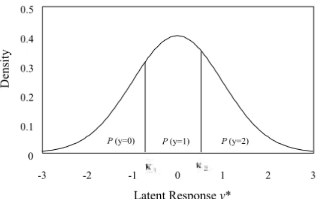
where k1i ,...,ksi are the threshold parameters for item i. Figure 1 illustrates this threshold model, which has three categories (S = 2). The areas under the curve are the probabilities of the observed responses. Dichotomous observed responses are a special case where S = 1.

Nonlinear Structural Equation Modeling

In NSEM, as in conventional SEM, there are both a structural part and a measurement part. The structural part specifies the relationship among latent traits and covariates, and the measurement part specifies the relationship between latent responses and the underlying latent traits (Skrondal & Rabe-Hesketh, 2004).

Structural Part

Let n index units or subjects. The structural model for latent traits _{n can be} specified as

(5)

where

α

is an intercept vector, B is a matrix of structural parameters governing the relations among the latent traits, Γ is a regression parameter matrix for regressions of latent variables on observed explanatory variables

x

_1n, and

ς

ⁿ _{is a} vector of disturbances (typically multivariate normal with zero mean). Note that this model is defined as conditional on the observed explanatory variables

x

_1n. Unlike conventional SEMs where all observed variables are treated as responses,

n n n

n

α Bη Γ x ς

η   

₁



0 0.1 0.2 0.3 0.4 0.5

-3 -2 -1 0 1 2 3

Latent Response y*

Density

P (y=0) P (y=1) P (y=2)

Figure 1. Threshold model for ordinal responses with three categories

no distributional assumptions about

x

_1nare necessary (Muthén, 1984; Skrondal &

Rabe-Hesketh, 2004).

For simplicity, consider that a single _nrepresents some latent trait (e.g., ability or attitude). This latent variable is regressed on observed covariates (e.g., gender, ethnicity, and their interaction):

_nγ 'x_1n_n (6)

ς

_n

~ N ( 0 , ϕ )

(7) where

γ

is a row-vector of regression parameters, which is sometimes referred to as latent regression because the dependent variable is latent rather than observed (Adams, Wilson, & Wu, 1997; Andersen, 2004; Christensen, Bjorner, Kreiner, &

Petersen, 2004; Mislevy, 1984; Zwinderman, 1991).

Measurement Part

With the latent-response formulation, the relationship between latent

responses

y

^*_n and latent traits _n and observed predictors

x

_2nis defined as:

y

^*_n

 v  Λη

_n

 Kx

_2n

 ε

_n (8) where v is a vector of intercepts,  is a factor loading matrix, and

ε

_nis a vector of unique factors or measurement errors. Muthén and Muthén (2007) extended measurement models by including the term Kx2n, where K is a regression parameter matrix for the regression of

y

^*_non observed explanatory variables x2j. Usually either v or the first threshold k1 is set at zero for model identification.

The inclusion of x_2n can be useful. For instance, if x_2n are group memberships, the corresponding parameter matrix can be used to detect construct invariance across groups (Stark, Chernyshenko, & Drasgow, 2006), which is often called differential

item functioning in the IRT literature (Holland & Wainer, 1993). When

ε

nis a multivariate normal distribution, this model (Equation 8), combined with the threshold model (Equation 4), becomes a probit model.

Generalizations

To be flexible, the measurement model can take the form:

g ( μ

ⁿ

)  v  Λη

ⁿ

 Kx

²ⁿ (9) where

g

(⋅)is a vector of link functions to handle different response types (e.g., continuous or categorical observed responses ),

μ

n is a vector of conditional means of the responses given _n and

x

_2n, and the other quantities are defined as in Equation 8. The conditional models for the observed responses given _n are assumed to follow the exponential family of distributions. There are no explicit unique factors in the model because the variability of the responses for given values of



n.

x

2nis accommodated by the conditional response distributions. The responses are implicitly specified as conditionally independent given that the latent variables _{n .}

g

(⋅)can be a logit function or a probit function for ordinal responses, a log function for count data, or an identity function for continuous responses (Hardin & Hilbe, 2007). Many IRT models can be formulated with Equation 9, including the family of Rasch models, the 2PLM, the generalized partial credit model, and the GRM (Sheu, Chen, Su, & Wang, 2005; Tuerlinckx &

Wang, 2004). Unfortunately, the 3-paramter logistic model (Equation 1) and many IRT models cannot be formulated with Equation 9.

Take the 2PLM as an example, where a set of dichotomous items measure the same latent variable . Let yni denote the item response (scored as 0 or 1) for

person n on item i, and



_niis its expected value. Equation 9 can be expressed as:

n i i ni

ni

P

ni

y

y

P

  

 









 

 v λ

) 1 ( 1

) 1 log (

) (

logit (10)

where the logit link function is used and v1 can be set at 0 and1 at 1 for model identification. For more formulations of IRT models using Equation 9, the reader is referred to Tuerlinckx and Wang (2004).

Parameter Estimation

In theory, the parameters in NSEM can be estimated with the EM algorithm (Bock & Aitkin, 1981). Unfortunately, the EM algorithm becomes inefficient or even infeasible when models contain a high dimensionality, which is almost always the case in NSEM. To resolve the computational problem, a combination of the Bayesian approach and the Markov chain Monte Carlo (MCMC) method has been proposed, which does not involve the intensive numerical integration that is often needed in the EM algorithm.

The basic idea of the MCMC method is to define a (stationary) Markov chain

M

0, M1, M2, … with states Mk = (

θ ,

^k

ζ

^k ), and simulate observations (i.e., states) from the Markov chain. Let θ be the latent variables vector and

ζ

be the unknown free parameters vector. Under suitable regularity conditions (Lee et al., 2007;

Tierney, 1994 ), the distribution of Mk, will converge to the chain’s stationary distribution π (θ,

ζ

) as k grows. The behavior of the Markov chain is determined by the so-called transition kernel:

t

[(

θ

⁰ ,

ζ

⁰),(

θ

¹ ,

ζ

¹)]

P

[

M

_k1(

θ

¹ ,

ζ

¹)|

M

_k (

θ

⁰ ,

ζ

⁰)] (11) and the probability of moving from current state(

θ

⁰ ,

ζ

⁰)to a new state(

θ

¹ ,

ζ

¹) ^. The stationary distribution satisfies:

[( , ),( , )] [( , ) ( , )] ( ¹ , ¹)

,

1 1 0 0 1

1 0

0

ζ θ ζ θ ζ θ ζ θ ζ

ζ

θ

θ







 ^{t d}

(12)

If one is able to define the kernel

t

[(

θ

⁰ ,

ζ

⁰),(

θ

¹ ,

ζ

¹)] so that the stationary distribution π (θ,

ζ

) equals the posterior distribution, then after a certain “burn- in” stage, the distribution of Mk will be approximately equal to the posterior distribution so that one can make inferences about the parameters. In general, one can use the corresponding sample statistics from the stationary distribution to estimate the parameter. For example, one can calculate the expected a posteriori (EAP) by taking the corresponding sample averages of(

θ

^k ,

ζ

^k), k =1, 2, …, L.

Gibbs Sampling

A simple calculation of Equation 11 gives the transition kernel:

t

_G[(

θ

⁰ ,

ζ

⁰),(

θ

¹ ,

ζ

¹)]

P

(

θ

¹ |

ζ

¹,

X

)

P

(

ζ

¹ |

θ

¹,

X

) (13) which has the stationary distribution equal to the posterior distribution P(θ,

ζ

| X), where X is the observed data. Markov chains utilizing the transition kernel as constructed in Equation 13 are called Gibbs samplers, which were first introduced by Geman and Geman (1984). In Equation 13, the two factors

P

(

θ

¹ |

ζ

¹,

X

) and

P

(

ζ

¹ |

θ

¹,

X

)are called complete conditional distributions.

In the Gibbs sampling, one simulates observations of parameter(

θ

^k ,

ζ

^k) ^by consecutively drawing samples from the complete conditional distributions. In order to obtain the observation of(

θ

^k ,

ζ

^k), one needs to start from(

θ

^k-1 ,

ζ

^k-1), which takes two transition steps: (a) drawing

θ

^k from the complete conditional distribution

P

(

θ

|

ζ

^k1,

X

); and (b) drawing

ζ

^k from the complete conditional distribution

ζ

^k

P

(

ζ

¹ |

θ

^k,

X

).

The Gibbs sampler draws inferences about one set of parameters by

assuming the other parameters to be fixed and known. However, the Gibbs sampler adjusts the inferences on that set of parameters for uncertainty about the other set by iterating these steps to the desired size. Note that both P(θ|

ζ

, X) and P(

ζ

^{|θ, X)} are proportional to the joint distribution P(θ,

ζ

, X)= P(X | θ,

ζ

) P(θ,

ζ

):

 ^{X θ ζ θ ζ θ}

ζ θ ζ θ X X

ζ

θ P P d

P P P

) , ( ) ,

| (

) , ( ) ,

| ) (

, |

( ＝ (14)

 ^{X θ ζ θ ζ ζ}

ζ θ ζ θ X X

θ

ζ P P d

P P P

) , ( ) ,

| (

) , ( ) ,

| ) (

, |

( ＝ (15) Assuming a priori independence of θ and

ζ

, one finds P(θ|

ζ

, X)∝

P(X ζ

|θ, )

P(θ) and P( ζ

|θ, X)∝

P(X |θ, ζ

) P(

ζ

). Because the denominators in Equations 14 and 15, known as the normalizing constants, are required, the MCMC method is designed to simplify or circumvent the calculation of those constants.

In short, the MCMC method is a combination of the Markov chain and the Monte Carlo integration estimating procedure. The first step in this procedure is to use the Gibbs sampling or Metropolis-Hastings algorithm to generate a stationary distribution of the Markov chain. The second step, according to the Monte Carlo integration method, is to utilize the sample mean close to the population mean in order to obtain the final estimation.

The MCMC method has been implemented in the freeware WinBUGS (Spiegelhalter, Thomas, & Best, 2003), which provides a great deal of information about parameter estimates, including point estimates, confidence intervals, parameter estimation process for each sampling, chart of estimated parameters, and others. WinBUGS has been widely applied to general linear and nonlinear models for continuous and non-continuous data, including complicated IRT models (Cowles, 2004; Qiu, Song, & Tan, 2002; Sturtz, Ligges, & Gelman, 2005).

Mplus Estimation

In addition to WinBUGS, computer software like Mplus (Muthén & Muthén, 2007) or LISREL (Jöreskog & Sörbom, 2006) can be used to estimate parameters in NSEM. These computer programs often use multistage methods to estimate parameters in NSEM. At the first stage, the tetrachoric or polychoric correlations and thresholds are estimated. At the second stage, the asymptotic distribution of the estimates is derived. At the final stage, the structural relationships can be analyzed through a generalized least square method. However, the multistage approach is not statistically optimal because it does not consider information about individuals, whereas WinBUGS does.

Mplus contains a basic program and three additional modules. The basic program examines the continuous latent factors and random effects and covers factor analysis, path analysis, structural equation modeling, and growth modeling.

The three additional modules are a mixture add-on, a multilevel add-on, and a combination add-on, all of which allow users to select additional modules to meet their research goals. Mplus also provides examples for IRT analyses (Muthén &

Muthén, 2007).

For binary or ordinal variables, Mplus estimates the thresholds for categorical variables using maximum likelihood estimation in the first step; estimates a matrix of tetrachoric correlations or polychoric correlations between the latent responses (also called latent correlations) in the second step; and obtains a consistent estimation of the asymptotic covariance matrix of the latent correlations with a

weighted least square estimator in the third step. Mplus is very flexible insofar as any combination of categorical and continuous observed variables can be presented in the data. It is assumed that categorical variables are associated with continuous and normally distributed latent response variables. Non-normality data can be estimated with weighted least squares (WLS) via a class of discrepancy fun

ctions:

F

_WLS (

s



σ

)

W

^1(

s



σ

) (16) where

s

= vech(S) and  = vech (Σ) and are vectorized elements of the tetrachoric (or polychoric) correlation matrix S and the implied matrix Σ, respectively;

vech(⋅)operator arranges the1/2

s

(

s

+1)nonredudant elements of the matrix into a vector, s is the number of elements; W is a u × u matrix and is a consistent

estimation of the asymptotic covariance matrix of s, and

u

=1/2

s

(

s

+1). In Equation 16,

W

⁻¹is used to adjust parameter estimation and is thus called the correct weight matrix. Different estimation strategies use different correct weight matrices. Estimation methods like unweighted least square, generalized least square and maximum likelihood can be regarded as a special application of WLS.

WLS requires a very large sample; however, developments in the WLS- based estimation of structural model parameters under non-normality have resolved the sample size problem. For example, Satorra (1992) and Muthén (1993) developed a mean-adjusted WLS estimator (WLSM) and a mean- and variance- adjusted WLS estimator (WLSMV). Both estimation methods are available in Mplus. The basic idea behind the WLSM and WLSMV is that the matrix W is chosen to be an estimate of the asymptotic covariance matrix of the estimates, denoted as . W matrix requires inversion but does not. A Taylor expansion of the asymptotic covariance matrix of the estimates yields a distinction between

W and

 . Therefore, from a computations standpoint, W can be chosen as any matrix that is easy to invert (e.g., the identity matrix). Thus, a robust estimator can be developed that does not require extensive computations or a huge sample size.

A Monte Carlo study demonstrated that the robust WLS estimator is quite general in that it allows for a combination of binary, ordered polytomous and continuous outcome variables and allows for multiple-group analysis (Muthén, 1993).

The Plausible-Value Approach

The above modeling with WinBUGS or Mplus requires original item responses. In practice, original item responses may not always be accessible and only summarized second-hand data are provided. For example, the 1983- 1984 National Assessment of Educational Progress (NAEP) provided users a set of five plausible values (PV) to represent uncertainty in ability estimates for individual test-takers (Mislevy, Sheehan, Beaton, & Johnson, 1992). Since then, the PV approach has been widely used in large-scale surveys, including the Trends in International Mathematics and Science Study (TIMSS) and the Program for International Student Assessment (PISA).

PV can be included as either dependent or independent variables (or both) in linear models. Since there are often multiple PVs, multiple analyses should be conducted, that is, one analysis for each PV. The results of these separate analyses then are combined to yield a final estimate. Let

β

ˆ_m (βˆ_m1,βˆ_m2,...,βˆ_mp),　

m

1,...,

M

(17) denote a vector of p estimated parameters from the m-th PV (M = 5 in this case),

and Um denote a p × p variance-covariance matrix of

βˆ

_m . The point estimates for the p parameters are the mean estimates across M PVs :

 

1 ˆ βˆ ,..., ˆ βˆ

1

*p 1*

*







 ^M

m m

M β

β

(18)

The variance-covariance matrix of ˆβ ^*is:





 

  



 M

1 1 ˆ )

cov( β

^*

U

^*

B

(19)

where ^M

M

m m



 







1

*

U

U

(20)

  

       

       

       



























































 



 



M m

p mp m

p mp m

p mp

p mp m

m m

m

p mp m

m m

m

T m M

m m

M M

1

* 2

*2

* 2

*1

* 1

*

*2 2

* 2 2

* 2 1

* 1 2 2

* 1*

* 1 2

* 2 1 1

* 2 1 1

* 1

*

βˆ βˆ βˆ βˆ βˆ βˆ βˆ βˆ βˆ βˆ

βˆ βˆ βˆ βˆ βˆ

βˆ βˆ βˆ βˆ βˆ

βˆ βˆ βˆ βˆ βˆ βˆ βˆ βˆ βˆ

βˆ 1

1

ˆ ˆ ˆ 1 ˆ

1













 β

β β β B

(21)

Simulation Study 1: Parameter Recovery of NSEM

In Simulation Study 1, we were interested in a comparison of Bayesian and non-Bayesian approaches to NSEM. It was expected that both WinBUGS and Mplus would yield a good parameter recovery and WinBUGS (Bayesian approach) would be slightly more efficient than Mplus (non-Bayesian approach) in parameter recovery when the data information was weak (e.g., short tests) because WinBUGS considered prior information, whereas Mplus did not.

Design and Data Generation

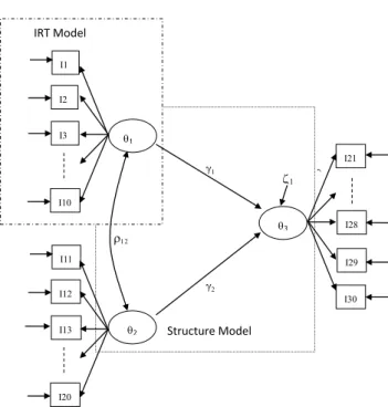
In the measurement part, the underlying IRT models were the 2PLM for dichotomous items and the GRM for 5-point items. In the structural part, there were two exogenous variables and one endogenous variable, each measured by a set of ten items following either the 2PLM or the GRM. Figure 2 presents the NSEM that was used in the simulation. The sample size was 1000; the test length was 10 items per latent trait; the two regression coefficients were 0.5 and 0.7;

and the correlation coefficient between the exogenous variables was .36. Under the 2PLM, the a-parameters ranged from 0.5 to 2.5, and the b-parameters ranged from -3 to 3. Under the GRM, the category thresholds were between -4 and 4. The examinees were generated from the standard normal distribution. The variances of the two exogenous variables were set at unity, and the residual variance of the endogenous variable was set at 0.25. The dependent variables were bias, root mean square error (RMSE), and relative efficiency in the estimates. The relative efficiency of Method A over Method B is defined as:

RE

A/B 

MSE

B/ MSEA (22) where MSE is the mean square error in the estimates. A value of RE^A/B greater than 1 indicates that Method A is more efficient than Method B.

A MATLAB 7.2 computer program was written by the authors for data generation, which consisted of the following steps:

1.The means and covariance matrix of the two exogenous variables were set according to the design.

2.Person parameters of the two exogenous variables were randomly generated from their multivariate normal distribution.

3.Person parameters of the endogenous variable were generated by multiplying its corresponding regression coefficients and adding the residual values.

4.Given the item and person parameters, the probabilities of item responses were computed according to the 2PLM or the GRM.

5. The cumulative probability was computed and compared to a number

Structure Model IRT Model

1

3

2

ε ε

λ

I1

I10 I2

…

I3

I11

I20 I12

…

I13

I30 I21

I29

…

I28

1

2



1

Figure 2. Graphic representation of a nonlinear structural equation model

randomly generated from the uniform distribution U(0, 1) to determine item score.

A total of ten replications were performed under each condition. Mplus 4.21 (Muthén & Muthén, 2007), with the default estimator of the robust maximum likelihood estimation, was used to estimate the parameters. To identify the parameters, the a-parameter of the first item for each latent trait was fixed at 1 and the mean of each latent trait was fixed at 0.The following normal priors were specified: bi ~ N(0, 4), dij ~ N(0, 4), ai ~ N(0, 4)I(0, ), where I(0, ) denotes an observation known to lie above zero; the prior for the two exogenous variances was set as inverted-Wishart (R[1;2, 1;2], 4), where R denotes a positive definite matrix and 4 is the degree of freedom; and the prior for the residual variance of the endogenous was set as inverted-Gamma (0.001, 0.001). The MCMC procedure had a run length of 5,000 iterations and a burn-in length of 1,000. These settings were similar to those used in the IRT literature (Béguin & Glas, 2001;

Bolt, Cohen, & Wollack, 2001; Bradlow, Wainer & Wang, 1999; Cowles, 2004;

Fryback, Stout, & Rosenberg, 2001; Kang & Cohen, 2007; Li et al., 2006; Raftery

& Lewis, 1996; Wang & Liu, 2007).

Results

Dichotomous Items. Parameter recovery of Mplus and WinBUGS is shown

in Tables 1 and 2, respectively. Mplus yielded a very good parameter recovery, with bias between -0.079 and 0.085, and RMSE between 0.040 and 0.222.

Likewise, WinBUGS yielded a very good parameter recovery, with bias between

-0.187 and 0.126, and RMSE between 0.027 and 0.204. The relative efficiency of WinBUGS over Mplus was between 0.30 and 8.39, with mean 1.61, indicating that WinBUGS was more efficient than Mplus, especially for the discrimination parameters.

Table1. Parameter recovery summary of NSEM with 10 dichotomous items per latent trait following the 2-parameter logistic model with Mplus in Study 1

a-parameter b-parameter

Item Gen Bias RMSE Gen Bias RMSE

θ1

1 1* 1.000 -0.044 0.088

2 0.806 0.025 0.117 -1.533 -0.001 0.123

3 0.456 0.035 0.072 -0.616 -0.010 0.077

4 1.045 0.011 0.200 1.141 -0.001 0.086

5 1.514 -0.025 0.160 0.354 -0.007 0.054

6 0.392 -0.024 0.083 -0.452 0.013 0.040

7 0.589 0.000 0.079 -0.310 0.000 0.063

8 1.604 0.036 0.168 1.771 0.000 0.145

9 0.722 0.037 0.108 0.694 0.019 0.063

10 1.249 0.057 0.176 1.516 0.025 0.124

θ2

11 1* 1.000 -0.059 0.099

12 1.310 0.085 0.182 0.339 0.029 0.083

13 0.557 0.079 0.155 -1.272 -0.050 0.076

14 1.169 -0.027 0.195 -1.724 0.006 0.138

15 1.664 0.004 0.175 -1.656 -0.021 0.153

16 1.511 0.083 0.222 -1.614 -0.079 0.155

17 0.561 -0.046 0.086 -0.187 -0.014 0.066

18 0.728 0.008 0.120 -0.211 0.003 0.065

19 1.265 0.035 0.165 0.199 0.011 0.072

20 0.401 -0.011 0.094 0.103 -0.015 0.043

θ3

21 22 23

1* 1.000 0.001 0.067

22 1.334 -0.067 0.120 0.891 -0.026 0.098

23 0.965 0.082 0.119 1.477 0.033 0.076

24 0.710 0.025 0.096 1.322 -0.007 0.064

25 0.523 0.017 0.087 -0.831 -0.006 0.088

26 1.354 0.085 0.109 0.370 -0.005 0.054

27 1.438 -0.063 0.093 1.208 -0.002 0.081

28 1.613 -0.079 0.125 1.202 0.015 0.147

29 1.199 0.072 0.139 1.781 0.021 0.082

30 0.786 -0.003 0.106 -0.950 0.020 0.064

γ1 0.500 0.020 0.068

γ2 0.700 0.026 0.092

 0.360 -0.036 0.085

Var1 1.000 -0.068 0.217

Var2 1.000 -0.063 0.173

Var3 0.250 -0.020 0.088

Note. *Fixed; Gen is generating value; RMSE is root mean square error; γ

1

is regression

coefficient of θ

3

on θ

1

; γ

2

is regression coefficient of θ

3

on θ

2

;

^

is correlation between θ

1

and θ

2

;

Var1 is the variance of θ

1

; Var2 is the variance of θ

2

; Var3 is the residual variance of θ

3

.

Table2. Parameter recovery summary of NSEM with 10 dichotomous items per latent trait following the 2-parameter logistic model with WinBUGS in Study 1

a-parameter b-parameter

Item Gen Bias RMSE Gen Bias RMSE

θ1

1 1* 1.000 -0.076 0.103

2 0.806 0.048 0.099 -1.533 -0.008 0.114

3 0.456 0.087 0.128 -0.616 -0.014 0.076

4 1.045 0.082 0.102 1.141 -0.009 0.069

5 1.514 0.057 0.073 0.354 0.014 0.048

6 0.392 0.051 0.100 -0.452 0.022 0.051

7 0.589 0.105 0.144 -0.310 -0.018 0.063

8 1.604 -0.006 0.058 1.771 -0.051 0.118

9 0.722 0.126 0.177 0.694 0.008 0.054

10 1.249 0.041 0.065 1.516 0.020 0.129

θ2

11 1* 1.000 -0.072 0.120

12 1.310 0.087 0.137 0.339 0.030 0.073

13 0.557 0.064 0.133 -1.272 -0.054 0.085

14 1.169 0.104 0.165 -1.724 -0.019 0.098

15 1.664 0.014 0.091 -1.656 -0.010 0.156

16 1.511 0.002 0.098 -1.614 -0.083 0.134

17 0.561 0.066 0.081 -0.187 -0.003 0.058

18 0.728 0.108 0.143 -0.211 -0.019 0.065

19 1.265 0.095 0.126 0.199 0.014 0.075

20 0.401 0.070 0.130 0.103 0.001 0.038

θ3

21 22 23

1* 0.000 1.000 -0.057 0.079

22 1.334 0.056 0.108 0.891 -0.002 0.064

23 0.965 0.084 0.142 1.477 -0.001 0.027

24 0.710 0.087 0.133 1.322 -0.002 0.059

25 0.523 0.063 0.098 -0.831 -0.031 0.071

26 1.354 0.091 0.109 0.370 -0.003 0.083

27 1.438 0.033 0.073 1.208 -0.033 0.095

28 1.613 0.002 0.089 1.202 -0.010 0.124

29 1.199 0.082 0.130 1.781 0.029 0.115

30 0.786 0.088 0.134 -0.950 0.012 0.059

γ1 0.500 0.036 0.063

γ2 0.700 0.029 0.078

 0.360 -0.059 0.101

Var1 1.000 -0.187 0.199

Var2 1.000 -0.172 0.204

Var3 0.250 -0.030 0.076

Note. *Fixed; Gen is generating value; RMSE is root mean square error; γ

1

is regression

coefficient of θ

3

on θ

1

; γ

2

is regression coefficient of θ

3

on θ

2

;

^

is correlation between θ

1

and θ

2

;

Var1 is the variance of θ

1

; Var2 is the variance of θ

2

; Var3 is the residual variance of θ

3

.

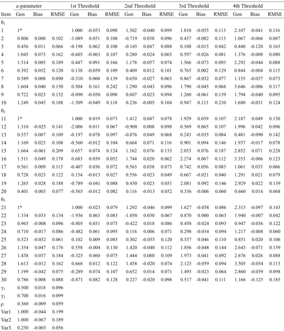
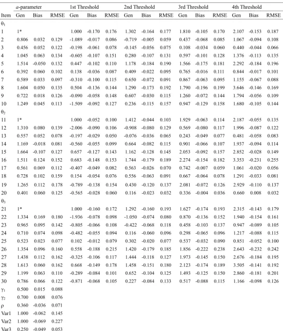
Polytomous Items. Parameter recovery of Mplus and WinBUGS is shown

in Tables 3 and 4, respectively. Mplus yielded a good parameter recovery, with bias between -0.125 and 0.161, and RMSE between 0.027 and 0.242. Likewise, WinBUGS yielded a good parameter recovery, with bias between -0.230 and 0.169, and RMSE between 0.032 and 0.255. The relative efficiency of WinBUGS over Mplus was between 0.07 and 6.10, with mean 0.99, indicating that these two programs had almost identical efficiency.

In summary, both WinBUGS and Mplus yielded a good parameter recovery for NSEM with dichotomous and polytomous items. WinBUGS was more efficient than Mplus in dichotomous items but they were similar in polytomous items, which was mainly because the priors played a relatively more important role than the data likelihood when there were only ten dichotomous items per latent trait, whereas the contribution of the priors became less important when there were ten 5-point polytomous items per latent trait. The computer time for Mplus was approximately one half of that for WinBUGS.

Table 3. Parameter recovery summary of NSEM with 10 five-point items per latent trait following the graded response model with Mplus in Study 1

a-parameter 1st Threshold 2nd Threshold 3rd Threshold 4th Threshold Item Gen Bias RMSE Gen Bias RMSE Gen Bias RMSE Gen Bias RMSE Gen Bias RMSE θ1

1 1* 1.000 -0.053 0.098 1.302 -0.040 0.099 1.810 -0.055 0.113 2.107 -0.041 0.116 2 0.806 0.000 0.102 -1.089 0.051 0.108 -0.719 0.038 0.096 0.437 -0.082 0.113 1.067 -0.066 0.087 3 0.456 0.011 0.066 -0.198 0.062 0.108 -0.145 0.047 0.088 0.108 -0.015 0.042 0.440 -0.120 0.163 4 1.045 0.073 0.162 -0.605 -0.063 0.107 0.280 -0.024 0.065 0.597 -0.026 0.081 1.376 -0.008 0.080 5 1.514 0.005 0.189 0.447 0.091 0.166 1.178 -0.057 0.074 1.566 -0.073 0.093 2.292 -0.044 0.088 6 0.392 0.052 0.120 0.138 -0.059 0.109 0.409 0.012 0.101 0.765 0.002 0.129 0.844 -0.004 0.115 7 0.589 0.008 0.090 -0.310 0.060 0.139 0.650 -0.027 0.063 0.867 -0.032 0.077 1.155 -0.037 0.073 8 1.604 0.040 0.150 0.504 0.161 0.242 1.290 -0.043 0.096 1.790 -0.045 0.068 3.646 -0.006 0.117 9 0.722 0.023 0.132 -0.090 -0.050 0.098 0.607 -0.023 0.094 1.260 -0.061 0.139 1.794 -0.040 0.095 10 1.249 0.045 0.188 -1.509 -0.049 0.118 0.236 -0.005 0.104 0.947 0.113 0.210 1.680 -0.031 0.124 θ2

11 1* 1.000 0.019 0.073 1.412 0.047 0.078 1.929 0.039 0.107 2.187 0.049 0.130 12 1.310 -0.025 0.141 -2.006 0.011 0.067 -0.908 0.008 0.098 0.569 0.065 0.107 1.996 0.042 0.096 13 0.557 0.007 0.109 -0.197 0.078 0.097 -0.076 0.049 0.068 0.243 -0.035 0.084 0.481 -0.090 0.142 14 1.169 0.023 0.108 -0.560 -0.012 0.104 0.664 0.071 0.116 0.901 0.094 0.146 1.937 -0.017 0.078 15 1.664 -0.061 0.209 0.657 0.074 0.124 1.162 0.076 0.133 2.053 0.076 0.187 2.852 0.071 0.228 16 1.511 0.049 0.178 0.683 0.039 0.052 1.744 0.020 0.062 2.274 0.067 0.112 3.353 -0.006 0.123 17

18 0.561 0.728

0.009 0.023

0.115 0.122

-0.407 0.154

0.036 -0.013

0.072 0.027

0.563 0.556

0.038 -0.023

0.073 0.049

0.742 0.667

0.056 -0.021

0.083 0.040

1.061 1.291

0.033 0.021

0.066 0.079 19 1.265 0.028 0.188 -0.789 -0.041 0.088 0.430 0.023 0.051 2.081 0.092 0.146 2.929 0.022 0.139 20 0.401 0.003 0.077 -0.565 -0.012 0.082 0.116 -0.013 0.052 0.336 -0.006 0.060 0.660 0.014 0.068 θ3

21 1* 1.000 -0.023 0.079 1.292 -0.046 0.099 1.627 -0.058 0.086 2.315 -0.097 0.143 22 1.334 0.033 0.134 -1.936 0.063 0.083 -1.050 0.030 0.067 0.870 0.000 0.063 1.940 -0.007 0.042 23 0.965 -0.008 0.096 -0.805 0.031 0.075 -0.422 0.018 0.086 0.458 -0.024 0.093 0.947 -0.036 0.122 24 0.710 -0.017 0.086 -0.482 0.061 0.095 0.116 0.006 0.071 0.298 -0.034 0.094 1.217 -0.008 0.060 25 0.523 -0.032 0.061 0.102 0.009 0.085 0.302 -0.055 0.120 0.537 0.046 0.110 0.851 0.020 0.106 26 1.354 0.047 0.176 0.558 -0.004 0.130 1.420 -0.040 0.112 1.856 -0.048 0.144 2.643 -0.071 0.159 27 1.438 0.037 0.184 -0.325 0.060 0.075 1.444 0.080 0.109 1.973 0.041 0.092 2.676 0.026 0.088 28 1.613 -0.012 0.162 0.668 0.012 0.122 1.458 -0.020 0.074 2.123 -0.059 0.094 3.505 -0.054 0.113 29 1.199 -0.042 0.075 -0.289 0.074 0.107 0.652 0.014 0.071 1.493 -0.023 0.064 2.860 -0.039 0.098 30 0.786 0.008 0.088 -0.871 0.082 0.128 0.227 -0.020 0.096 0.517 -0.041 0.111 1.166 -0.125 0.185 γ1 0.500 0.018 0.096

γ2 0.700 0.016 0.099

 0.360 -0.009 0.059 Var1 1.000 -0.044 0.199 Var2 1.000 -0.067 0.189 Var3 0.250 -0.003 0.056

Note. *Fixed; Gen is generating value; RMSE is root mean square error; γ

1

is regression

coefficient of θ

3

on θ

1

; γ

2

is regression coefficient of θ

3

on θ

2

;

^

is correlation between θ

1

and θ

2

;

Var1 is the variance of θ

1

; Var2 is the variance of θ

2

; Var3 is the residual variance of θ

3

.

Table 4. Parameter recovery summary of NSEM with 10 five-point items per latent trait following the graded response model with WinBUGS in Study 1

19 1.265 0.112 0.178 -0.789 -0.138 0.154 0.430 -0.120 0.137 2.081 -0.072 0.126 2.929 -0.110 0.137 20 0.401 0.060 0.125 -0.565 -0.028 0.060 0.116 -0.023 0.032 0.336 -0.004 0.036 0.660 0.008 0.032 θ3

21 1* 1.000 -0.160 0.172 1.292 -0.160 0.193 1.627 -0.174 0.193 2.315 -0.143 0.179 22 1.334 0.169 0.180 -1.936 -0.078 0.098 -1.050 -0.074 0.080 0.870 -0.136 0.152 1.940 -0.154 0.161 23 0.965 0.095 0.142 -0.805 -0.066 0.108 -0.422 -0.068 0.118 0.458 -0.103 0.137 0.947 -0.089 0.105 24 0.710 0.074 0.098 -0.482 -0.055 0.094 0.116 -0.060 0.096 0.298 -0.065 0.096 1.217 -0.088 0.115 25 0.523 0.023 0.077 0.102 -0.012 0.079 0.302 -0.020 0.077 0.537 -0.032 0.090 0.851 -0.052 0.100 26 1.354 0.096 0.160 0.558 -0.188 0.215 1.420 -0.179 0.185 1.856 -0.222 0.238 2.643 -0.232 0.242 27 1.438 0.112 0.162 -0.325 -0.106 0.117 1.444 -0.118 0.127 1.973 -0.145 0.150 2.676 -0.184 0.195 28 1.613 0.060 0.162 0.668 -0.149 0.178 1.458 -0.151 0.180 2.123 -0.174 0.189 3.505 -0.141 0.192 29 1.199 0.063 0.110 -0.289 -0.084 0.101 0.652 -0.104 0.125 1.493 -0.125 0.150 2.860 -0.181 0.201 30 0.786 0.066 0.122 -0.871 -0.068 0.105 0.227 -0.084 0.133 0.517 -0.088 0.115 1.166 -0.098 0.126 γ1 0.500 0.015 0.088

γ2 0.700 0.008 0.076

 0.360 -0.036 0.071 Var1 1.000 -0.062 0.145 Var2 1.000 -0.069 0.227 Var3 0.250 -0.049 0.053

Note. *Fixed; Gen is generating value; RMSE is root mean square error; γ

1

is regression coefficient of θ

3

on θ

1

; γ

2

is regression coefficient of θ

3

on θ

2

;

^

is correlation between θ

1

and θ

2

; Var1 is the variance of θ

1

; Var2 is the variance of θ

2

; Var3 is the residual variance of θ

3

.

a-parameter 1st Threshold 2nd Threshold 3rd Threshold 4th Threshold Item Gen Bias RMSE Gen Bias RMSE Gen Bias RMSE Gen Bias RMSE Gen Bias RMSE θ1

1 1* 0.000 1.000 -0.170 0.176 1.302 -0.164 0.177 1.810 -0.105 0.170 2.107 -0.153 0.187 2 0.806 0.032 0.129 -1.089 -0.017 0.086 -0.719 -0.005 0.059 0.437 -0.068 0.085 1.067 -0.094 0.108 3 0.456 0.052 0.122 -0.198 -0.061 0.078 -0.145 -0.056 0.075 0.108 -0.034 0.060 0.440 -0.044 0.066 4 1.045 0.063 0.134 -0.605 -0.107 0.151 0.280 -0.107 0.131 0.597 -0.101 0.128 1.376 -0.113 0.135 5 1.514 -0.050 0.132 0.447 -0.102 0.110 1.178 -0.184 0.190 1.566 -0.175 0.181 2.292 -0.184 0.196 6 0.392 0.060 0.102 0.138 -0.036 0.087 0.409 -0.022 0.095 0.765 -0.016 0.111 0.844 -0.017 0.101 7 0.589 0.033 0.097 -0.310 -0.100 0.115 0.650 -0.072 0.091 0.867 -0.063 0.095 1.155 -0.067 0.088 8 1.604 0.050 0.135 0.504 -0.136 0.144 1.290 -0.173 0.192 1.790 -0.196 0.199 3.646 -0.146 0.169 9 0.722 0.018 0.126 -0.090 -0.058 0.148 0.607 -0.030 0.115 1.260 -0.072 0.144 1.794 -0.056 0.109 10 1.249 0.045 0.113 -1.509 -0.092 0.127 0.236 -0.115 0.157 0.947 -0.129 0.158 1.680 -0.105 0.144 θ2

11 ^1* 1.000 -0.052 0.100 1.412 -0.044 0.103 1.929 -0.063 0.114 2.187 -0.055 0.135 12 1.310 0.080 0.139 -2.006 -0.090 0.106 -0.908 -0.080 0.129 0.569 -0.080 0.117 1.996 -0.087 0.122 13 0.557 0.052 0.078 -0.197 -0.029 0.050 -0.076 -0.036 0.065 0.243 -0.049 0.077 0.481 -0.058 0.083 14 1.169 -0.018 0.081 -0.560 -0.055 0.099 0.664 -0.082 0.115 0.901 -0.066 0.107 1.937 -0.094 0.114 15 1.664 -0.107 0.127 0.657 -0.127 0.143 1.162 -0.128 0.145 2.053 -0.092 0.157 2.852 -0.028 0.149 16 1.511 0.124 0.152 0.683 -0.148 0.153 1.744 -0.179 0.189 2.274 -0.154 0.182 3.353 -0.231 0.255 17 0.561 0.069 0.112 -0.407 -0.049 0.082 0.563 -0.026 0.070 0.742 -0.007 0.059 1.061 -0.020 0.056 18 0.728 0.102 0.159 0.154 -0.054 0.076 0.556 -0.063 0.091 0.667 -0.064 0.078 1.291 -0.033 0.081

Simulation Study 2: The PV Approach

In practice, original item responses may not be always accessible; in such cases, the above one-staged NSEM is not possible. Investigation of how the PV approach will recover the structural parameters in such a case is of great interest.

Design

The simulation design was very similar to that in Study 1, except we were interested in recovery of only the structural parameters. A set of five PVs were randomly sampled from WinBUGS. Next, five separate path analyses were performed, and their parameter estimates were combined using Equations 18 and 19. For comparison, the EAP and MLE derived from the computer programs BILOG-MG (for the 2PLM) and MULTILOG (for the GRM) were also used to conduct path analyses (visit http://www.assess.com/xcart/home.php?cat=26 for the two programs) using the software package SPSS. The test length was either 5 or 10 items per latent trait; the regression coefficients for the two exogenous variables were 0.5 and 0.7; and the correlation coefficient between the two exogenous variables was .36. Under the 2PLM, the a-parameters ranged from 0.5 to 2.5, and the b-parameters ranged from -3 to 3. Under the GRM, the category thresholds of the 5-point items were between -4 and 4. A total of 1000 examinees were generated from the standard normal distribution. The variances of the two exogenous variables were set at unity, and the residual variance of the endogenous variable was set at 0.25.

It was expected that the PV approach would recover the structural parameters

fairly well, and the results would be very similar to those found in Simulation Study 1 where Mplus and WinBUGS were applied to analyze original item responses. The EAP or MLE approach would underestimate the magnitudes of the structural parameters because measurement error in person parameters was ignored completely—the shorter the test, the larger the measurement error in person measure, and the worse the EAP and MLE approach would perform.

Results

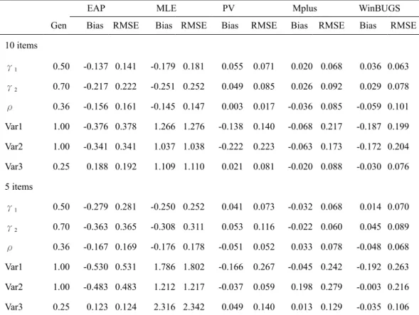
Table 5 reports the parameter recovery for the PV approach in the dichotomous items, in comparison of EAP, MLE, Mplus and WinBUGS. As expected, the PV approach yielded a small bias and a small RMSE, which were very similar to those obtained from Mplus and WinBUGS. On the contrary, the EAP approach substantially underestimated the two regression parameters, the correlation between exogenous variables, and the variances of the two exogenous variables, but it overestimated the residual variance of the endogenous variable. The MLE approach substantially underestimated the two regression parameters and the correlation between exogenous variables, but it overestimated the variances of the two exogenous variables and the residual variance of the endogenous variable. The biased estimation for the EAP and MLE approaches was more serious when the test was short (i.e., 5 dichotomous items per latent trait).

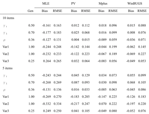
The parameter recovery of polytomous items is shown in Table 6. The EAP approach was not applicable because MULTILOG did not produce EAP. As found in the dichotomous items comparison, the PV approach performed very similarly