機器手掌與機器手臂自動抓取規劃與軌跡規劃

國立臺灣大學工學院機械工程學研究所 碩士論文

Department of Mechanical Engineering College of Engineering

National Taiwan University Master Thesis

機器手掌與機器手臂自動抓取規劃與軌跡規劃 Automated Grasp Planning and Path Planning for a Robot

Hand-Arm System

劉貽仁 Yi-Ren Liu

指導教授：黃漢邦博士 Advisor: Han-Pang Huang, Ph.D.

中華民國 105 年 7 月

July 2016

誌謝

忙碌的碩士生涯很快就要邁入尾聲，這兩年的時間裡讓我受益良多。

首先，要感謝我的家人，一直在背後默默地支持著我，為我加油打氣，讓我 無後顧之憂的完成學業；感謝指導教授黃漢邦老師在研究上給予的指導與資源，

讓我在這兩年學到了許多，對於日後必定有很大的幫助；也感謝口試委員林錫寬 教授、曾清秀教授與黃國勝教授在口試中給予許多的經驗與建議。

再來，我要感謝實驗室的朋友們。感謝聖諺、明寶、志豪、威志、煥坤及相 元學長，謝謝你們教會我許多實驗室的軟硬體基礎架構並且在我的研究上給予許 許多多寶貴意見。感謝世全、建興、尚庭、俊傑、劍航、鼎元和逸祥，不管是在 學習或生活，謝謝你們陪伴我一起奮鬥；也感謝學弟們的幫助，尤其是家豪與浩 雲。幫助我許多。在實驗室的時光，有你們這群朋友真好。也相信實驗室有你們 在會更加興盛。

再次感謝所有幫助我的每一個人。

2016/7/21 於台大機器人實驗室

摘要

多指機器手掌抓取物體的分析，一直是機器人研究中十分重要的研究議題。

日常生活中，物體並不會是個簡單的幾何形狀，例如方形、圓形、圓柱、錐形。

而是像馬克杯、小花瓶、清潔劑等，較為複雜的形狀。而多指機器手掌的自由度 比起機器夾爪多了許多，找到有效的抓取點就變得十分重要。因此，本論文旨在 探討如何在複雜幾何的物體上利用力旋量空間尋找多指機器手掌可抓取的姿態以 及根據物體邊界盒限制機器手臂可到達的區域加速找到一組可以抓取的最終姿態。

再以阻尼最小平方法解決逆運動學中奇異點問題，並且在六軸機器手臂軸空間中，

利用兩棵快速擴展隨機樹連接法尋找避開障礙物的路徑。並透過三維點雲進行點 雲處理並重建環境以及物體表面模型，以達到自動化抓取的目標。

關鍵字：機器手臂、機器手掌、抓取規劃、軌跡規劃、表面重建。

Abstract

Analysis of a multi-fingered robot hand for grasping objects is an important research issue in robotics. Objects in daily life are not simple geometric shape like square, spherical, cylindrical, conical shapes. Most are the complex geometric shapes.

Since the number of degrees of freedom of a multi-fingered robot hand is more than the simple gripper, it is important to find the grasping points. This thesis mainly focuses on how to determine the grasping points on the complex geometric shapes with the multi-fingered robot hand. Each grasping can be described by grasp wrench space (GWS). The quality measure can be determined from analyzing the GWS. The bounding box of object is a constraint on the workspace of the robot hand-arm system.

According to the constraints, the random based algorithm can speed up the searching speed. The damped least square (DLS) method is use for solving the inverse kinematics problem about singular points. The rapidly-exploring random trees (RRT) – connect algorithm is used to search for the collision-free path in the joint space of the robot arm.

The point cloud can be processed by point cloud processing and surface reconstruction.

It combines the real environment and simulation. The goal can be reached through these methods.

Keywords: Robot Hand-Arm System, Grasp Planning, Path Planning, Surface Reconstruction.

Contents

誌謝 ...i

摘要 ... ii

Abstract ... iii

List of Tables ... vii

List of Figures ... viii

Chapter 1 Introduction ... 1

1.1 Motivation... 1

1.2 Contributions ... 2

1.3 Organization ... 3

Chapter 2 Kinematics ... 5

2.1 Introduction... 5

2.2 Forward Kinematics... 6

2.2.1 Transformation Matrix ... 6

2.2.2 Kinematic Chain ... 7

2.2.3 Denavit-Hartenberg (DH) Convention ... 7

2.2.4 Forward Kinematics ... 10

2.2.5 Forward Kinematics of Multiple End-Effectors... 11

2.3 Inverse Kinematics Algorithms ... 12

2.3.1 Jacobian Matrix ... 13

2.3.2 The Jacobian Transpose Method ... 16

2.3.3 The Pseudoinverse Method ... 16

2.3.4 Damped Least Square (DLS) Method ... 18

Chapter 3 Grasp Analysis and Synthesis ... 25

3.1 Introduction... 25

3.2 Background ... 25

3.2.1 Contact Kinematics ... 25

3.2.2 Contact Models ... 27

3.2.3 Friction Cone ... 29

3.2.4 Grasp Wrench Space ... 30

3.3 Grasp Quality Measure ... 33

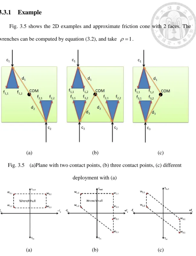
3.3.1 Example ... 35

3.4 Grasp Planning... 37

Chapter 4 Path Planning ... 41

4.1 Introduction... 41

4.2 Rapidly-Exploring Random Trees ... 42

4.2.1 The Basic RRT algorithm ... 43

4.2.2 The RRT-Connect Algorithm ... 47

4.3 Path Pruning Algorithm ... 49

4.4 Planning Algorithm ... 51

4.4.1 Path Planning Algorithm ... 51

4.4.2 Grasp with Path Planning Algorithm ... 51

4.5 Summary ... 52

Chapter 5 Object Reconstruction ... 55

5.1 Introduction... 55

5.2 Point Cloud Processing ... 56

5.2.1 Pass Through Filter ... 56

5.2.2 Down-Sampling ... 57

5.2.3 Random Sample Consensus ... 58

5.2.4 Euclidean Segmentation ... 59

5.3 Surface Reconstruction ... 61

Chapter 6 Simulations and Experiments ... 65

6.1 Hardware Platform... 65

6.1.1 Six-DOF Robot Arm ... 65

6.1.2 NTU Robotic Hand V ... 66

6.1.3 Sensors ... 69

6.2 Software Platform ... 71

6.3 Simulation Results and Experiment Demonstrations ... 73

6.3.1 Grasping Results: Ball ... 76

6.3.2 Grasping Results: Bottle ... 78

6.3.3 Grasping Results: Joystick ... 79

Chapter 7 Conclusions and Future Works ... 81

7.1 Conclusions ... 81

7.2 Future Works ... 82

References ... 83

List of Tables

Table 3.1 The grasp planning algorithm ... 39

Table 4.1 The basic RRT algorithm ... 44

Table 4.2 The RRT-Connect algorithm ... 47

Table 4.3 Path pruning algorithm ... 50

Table 4.4 Path Planning Algorithm ... 51

Table 4.5 Grasp with Path Planning Algorithm ... 52

Table 6.1 Specifications of NTU Arm ... 65

Table 6.2 Specification of NTU-Hand V ... 67

List of Figures

Fig. 2.1 Representation of a point P in different coordinate frames [51] ... 6

Fig. 2.2 Open kinematic chain ... 7

Fig. 2.3 Denavit-Hartenberg kinematic parameters ... 7

Fig. 2.4 Joint frame relation of the NTU Arm ... 9

Fig. 2.5 Joint relation using the tree to construct ... 9

Fig. 2.6 Joint frame relation of the NTU-Hand V ... 10

Fig. 2.7 Joint frame relation of the arm-hand system ... 10

Fig. 2.8 Multiple end-effectors examples [51] ... 12

Fig. 2.9 The relation between joint i and the end-effector i [51] ... 14

Fig. 2.10 The error e choose in each iteration ... 15 _i Fig. 2.11 Test example ... 20

Fig. 2.12 The Jacobian transpose method ... 20

Fig. 2.13 The pseudoinverse method ... 20

Fig. 2.14 The DLS method... 21

Fig. 2.15 Test example ... 22

Fig. 2.16 The Jacobian transpose method ... 22

Fig. 2.17 The pseudoinverse method ... 22

Fig. 2.18 The DLS method... 23

Fig. 3.1 Notation for an object in contact [9] ... 26

Fig. 3.2 Three common contact models used in robot grasping [9]... 28 Fig. 3.3 Friction cone:(a) spatial representation, (b) approximation representation.

Fig. 3.4 A sample 3 contact on a planar object. [15]... 31

Fig. 3.5 (a)Plane with two contact points, (b) three contact points, (c) different deployment with (a) ... 35

Fig. 3.6 GWS corresponding to Fig. 3.5 (a)(b)(c)... 35

Fig. 3.7 (a)Q quality measure for Fig. 3.5 (b), (b)₁ Q quality measure for ₁

Fig. 3.5 (c)... 36

Fig. 3.8 Quality measure examples with a simple ball ... 36

Fig. 3.9 Example of AABB ... 37

Fig. 3.10 Random sampling of the robot arm. ... 38

Fig. 3.11 The example of robot hand grasp ... 38

Fig. 4.1 The extend(T, q ) function [27] ... 44

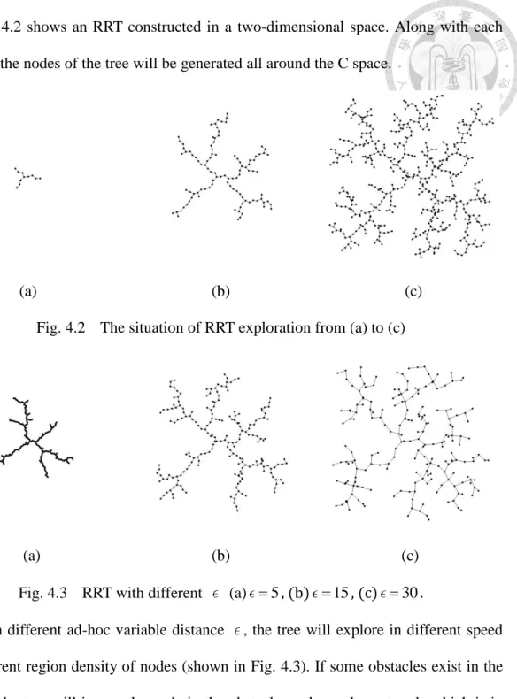
Fig. 4.2 The situation of RRT exploration from (a) to (c)... 45

Fig. 4.3 RRT with different (a) 5, (b) 15, (c) 30. ... 45

Fig. 4.4 RRT in the C-space with an obstacle. (a) Small , (b) Large . ... 46

Fig. 4.5 From start configuration to goal configuration (a) all vertices, (b) the path.47 Fig. 4.6 From start configuration to goal configuration without obstacles ... 48

Fig. 4.7 From start configuration to goal configuration (a) all vertices (b) the path. 48 Fig. 4.8 High dimension C space example (a) start configuration, (b) goal configuration. ... 49

Fig. 4.9 From start point to goal point (a) all vertices, (b) the path. ... 49

Fig. 4.10 (a) Original path, (b) the path through path pruning algorithm. ... 51

Fig. 4.11 The path (a) not consider the target, (b) consider the target. ... 52

Fig. 4.12 The path (a) not consider the table, (b) consider the table... 53

Fig. 4.13 The path (a) not consider the obstacles, (b) consider the obstacles. ... 53

Fig. 5.2 3D Imaging (a) Real environment, (b) point cloud from the depth sensor. .. 56

Fig. 5.3 Raw data of point cloud set ... 57

Fig. 5.4 The output of pass through filter ... 57

Fig. 5.5 Down-sampling algorithm (a) original point cloud, (b) after down-sampling. ... 58

Fig. 5.6 RANSAC algorithm (a) Original point cloud, (b) The plane search by RANSAC. ... 59

Fig. 5.7 Segmentation (a) Original point cloud, (b) after segmentation. ... 61

Fig. 5.8 Example of PCA. ... 62

Fig. 5.9 Surface Normal estimation. ... 62

Fig. 5.10 A quadratic function fitted on a set of data. ... 63

Fig. 5.11 Resampling and Surface Normal estimation. ... 63

Fig. 5.12 The example of surface reconstruction. ... 64

Fig. 6.1 NTU Arm with six DOFs. ... 65

Fig. 6.2 Overall System for Hand System. ... 66

Fig. 6.3 NTU five fingers hand. ... 66

Fig. 6.4 The under-actuated robotic finger. ... 68

Fig. 6.5 SEA mechanism. ... 69

Fig. 6.6 The electrical model of FSR. ... 70

Fig. 6.7 The tactile sensor. ... 70

Fig. 6.8 The Microsoft Kinect XBOX 360 device. ... 70

Fig. 6.9 Collision detection example. ... 71

Fig. 6.10 The GUI of robot simulator. ... 72

Fig. 6.11 The experimental environment. ... 73

Fig. 6.13 The detail of point cloud block. ... 74 Fig. 6.14 Objects (a) on real table, (b) point cloud, (c) simulator. ... 75 Fig. 6.15 The detail of the robot simulator block... 75 Fig. 6.16 The ball and the reconstructed surface. ... 76 Fig. 6.17 The Q₁ quality measure and final pose of robot in experiment 1. ... 76 Fig. 6.18 The procedure of experiment 1. ... 77 Fig. 6.19 The bottle and the reconstructed surface. ... 78 Fig. 6.20 The Q₁ quality measure and final pose of robot in experiment 2. ... 78 Fig. 6.21 The path planning: (a) to grasp (b) to place. ... 78 Fig. 6.22 The procedure of experiment 2. ... 79 Fig. 6.23 The joystick and the reconstructed surface. ... 80 Fig. 6.24 The Q₁ quality measure and final pose of robot in experiment 3. ... 80 Fig. 6.25 The procedure of experiment 3. ... 80

Chapter 1 Introduction

1.1 Motivation

Robots are becoming increasingly important in daily life. To make our lives more convenient, humans use technology to create robots for service tasks involving fetching or transporting objects. In the tasks that require object acquisition, the pick-and-place motion is performed by an autonomous manipulator. Within the surfaces of the desired placement for picking, it is important to operate a direct reach-to-pick to achieve object acquisition; however, in an unstructured environment or one that is not designed for the purpose and where the object placement may be changeable, the motion of a direct reach-to-pick may not be always convenient for object picking. Therefore, the ability required for efficient object picking is worthy of discussion. This thesis is inspired by the following three motivations.

First, in the industry field, robots with six joints and single DOF end effector are typically used to grip objects. For specific environment, industrial robots with grippers can achieve fast and accurate manipulation action for object picking because the grippers are lightweight and easy to control. However, grippers cannot perform fine manipulation or adapt to an unstructured environment. Therefore, we use multi-fingered robot hands with multiple DOFs and multiple joints to realize precise placement and adaptation.

Second, visual perception plays an important role in the interaction between the robot hand and the object for manipulating tasks. Vision is used not only to obtain relevant information about the objects such as position and orientation but also to reduce the uncertainty of achieving precise contact. With information about the objects,

using vision sensors to detect the objects and the environment, we can make object grasping more robust.

Third, even though the multi-fingered robot hand has more degrees of freedom than gripper, without the strategy which determines the suitable contact points, the benefit of multi-fingered robot hand cannot come out. With classical theory of the robot hand, there is a fast algorithm to evaluate the grasp quality. The quality score is generated from the physical meaning of human-like motion. This is convenient to find appropriate contact points with some random base pose generator.

With these three motivations, we integrate some methods and use a multi-fingered hand and a robotic arm system to perform the object grasping.

1.2 Contributions

This thesis attempts to develop the strategy of a grasp planning and path planning system to grasp arbitrary objects in an unstructured environment. Four main contributions of this thesis are as follows:

 Use a quality measure to score the grasp points and create a random based pose generator which easily searches for the grasp points for the robot arm-hand system.

 Use the RRT-Connect algorithm in the high-dimensional configuration space to find the collision free path from an initial configuration to goal configuration.

 Use point cloud processing to reconstruct the object surface and combine the real environment and simulation environment.

1.3 Organization

The remainder of this thesis is organized as follows.

Chapter 2 introduces the basic kinematics of robotics. Kinematics describes the frame relationship. The robot hand frame model is different from the robot arm. The branch part and the passive joint part will be considered. Jacobian computation and different inverse kinematics algorithms will be addressed. The kinematics is the basis of many applications like workspace, collision detection, etc.

Chapter 3 is scoring the grasping from a physical viewpoint. In recent researches the grasping quality is usually measured from learning viewpoint, but must with the completely physical simulator. In physical viewpoint, the grasping is explored mainly from friction cones. The grasp wrench and the determination of the final configuration of the robot arm-hand system will be discussed. With the fast quality measure computation, the random based pose generator can deal with this problem well.

Chapter 4 presents the searching path problem. Path planning is the other important issue in robotics. To search for the collision free path, we use the RRT-Connect in the configuration space.

Chapter 5 introduces several point cloud processing methods. The depth sensor can easily collect the 3D environment information. But there exist problems about the point cloud, such as noise, low precision, many unnecessary points. The point cloud is used to reconstruct the object surface.

Chapter 6 presents the simulation results and experiment results. Conclusions and future works are given in Chapter 7.

Chapter 2 Kinematics

2.1 Introduction

Kinematics describes the relation about all frames which are used to describe the joints in robot system. With this relation in simulation, it can help to detect collision if the link has self-collision information like CAD model in simulator, because the location about every joint and link are known. The end-effector of the robot arm is important information, and can help the palm of the robot hand to determine the pre-grasp pose.

On the other hand, inverse kinematics (IK) determines the corresponding joint space values that can move the end-effector to the goal described in base frame.

This chapter presents forward kinematics and inverse kinematics. Some inverse kinematics algorithms are widely used in the robotics, such as cyclic coordinate descent methods [57], pseudoinverse methods [58], Jacobian transpose methods [7, 59], the Levenberg-Marquardt damped least squares methods [38, 56], quasi-Newton and conjugate gradient methods [57], and neural net and artificial intelligence methods [43].

This thesis focuses on the iteration method of IK.

2.2 Forward Kinematics 2.2.1 Transformation Matrix

As shown in Fig. 2.1, consider an arbitrary point p in the space. Let p⁰ ³ be the vector of P with respect to the reference frame O , and ₀ p¹ ³ with respect to the reference frame O . ₁ p and ⁰ p have the relation: ¹

0 0 0 1

1 1

p o R p

0 0 0 1

0 1 1 0 1

1 0^T 1 1 1

p R o p

p       T p

     

      (2.1)

0 3

o1  is the origin of Frame 1 with respect to Frame 0, and R1⁰ ^{3 3} SO

 

 

Fig. 2.1 Representation of a point P in different coordinate frames [51]

It is easy to verify that a sequence of coordinate transformations can be composed of the product as

0 0 1 1

1 2... _n^{n n}

p T T T ^ p (2.2)

where T_i^i1 denotes the transformation relating a point in Frame i to the same point in Frame i1.

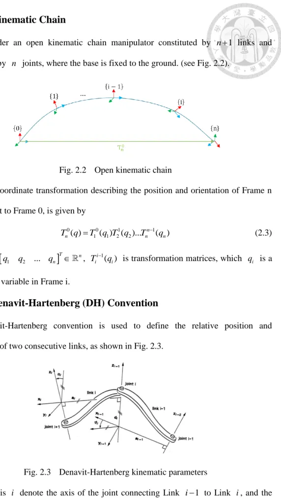
2.2.2 Kinematic Chain

Consider an open kinematic chain manipulator constituted by n1 links and connected by n joints, where the base is fixed to the ground. (see Fig. 2.2).

Fig. 2.2 Open kinematic chain

Then, the coordinate transformation describing the position and orientation of Frame n with respect to Frame 0, is given by

0 0 1 1

1 1 2 2

( ) ( ) ( )... ⁿ ( )

n n n

T q T q T q T ^ q (2.3)

where q





2.2.3 Denavit-Hartenberg (DH) Convention

Denavit-Hartenberg convention is used to define the relative position and orientation of two consecutive links, as shown in Fig. 2.3.

Fig. 2.3 Denavit-Hartenberg kinematic parameters

Let axis i denote the axis of the joint connecting Link i1 to Link i , and the

transformation matrix Ti^i1  f a





a : the shortest distance from i zˆ_i1 to ˆz , measured along ˆ_i x axis. _i

i:the offset angle from zˆ_i1measured about ˆx axis. _i

d :the shortest distance from i xˆ_i1 to ˆx , measured along _i zˆ_i1 axis.

i: the offset angle from xˆ_i1 measured about zˆ_i1 axis.

1

1 1

cos( ) sin( ) cos( ) sin( ) sin( ) cos( ) sin( ) cos( ) cos( ) sin( ) cos( ) sin( )

0 sin( ) cos( )

0 0 0 1

0 1

i i i i i i i

i i i i i i i

i i

i i i

i i

i i

T

a T a

d

R p

     

     

 



 

  

  

 

 

 

 

 

  

 

(2.4)

where Ri^i1 ^{3 3} ^{SO 3}

 

i , ^i1p_i ³ is the distance vector between Frame i and Frame i1 describe in Frame i1.

If the joint i is the revolute joint, T_i^i1 also the function of the joint value q : _i

1

1 1

cos( ) sin( ) cos( ) sin( ) sin( ) cos( )

sin( ) cos( ) cos( ) sin( ) cos( ) sin( )

( ) 0 sin( ) cos( )

0 0 0 1

( ) ( )

0 1

i i i i i i i i i i i

i i i i i i i i i i i

i

i i

i i i

i i

i i i i

T

q q q a q

q q q a q

T q

d

R q p q

     

     

 



 

    

 

      

 

 

 

 

 

  

 

(2.5)

The joint frame relation of the NTU Arm is shown in Fig. 2.4. Each frame will record the parent frame and the transformation matrix about the child frame. For the arm, the joint relation likes a linked list. To construction the joint frame relation for the robotic hand, the tree data structure is used store the joints (Fig. 2.5). The root of the tree is the robotic hand base as shown in Fig. 2.5 with as a red cycle. The children of the root are the first joint of each finger, and then the next DH construction is the same as the normal DH convention method. The final result is shown in Fig. 2.6. Hence, the robotic arm-hand system can be constructed using the tree data structure, as shown in Fig. 2.7.

Fig. 2.4 Joint frame relation of the NTU Arm

Fig. 2.5 Joint relation using the tree to construct

Fig. 2.6 Joint frame relation of the NTU-Hand V

Fig. 2.7 Joint frame relation of the arm-hand system

2.2.4 Forward Kinematics

The one end-effector robot like pure robot arm can use the method of section 2.2.2, 2.2.3 to derive the position and orientation of end-effector by solving the equation (2.3), and T q is the answer. _n⁰( )

Let s ⁶ be the Cartesian vector as

 

3 3

where

x y z

x y z

T T

e e e x y z e

T T

e e e e x y z

s p p p k k k p k

p p p p k k k k

 

  

   

     

(2.6)

Each finger of the robot hand can be treated as a robot arm. Therefore, we have

   

0 4 4

n 3

T q  ^ SE . Note that p is the position vector which equals to the _e ⁰p_n

(equation (2.4)) in T , and k is the orientation vector. _n⁰

0

R (equation (2.4)) in n T and k can be obtained as _n⁰

2.2.5 Forward Kinematics of Multiple End-Effectors

When the kinematic chain has separate branches in some nodes, the multiple end-effectors is generated (see Fig. 2.8). Let t denote the frame attached to the torso, r and l the base frames, respectively, of the right arm and the left arm, and rh and lh the frames attached to the two hands (end-effectors). It is possible to compute for the right arm and the left arm, respectively.

0 0 3

3

t r

rh t r rh

T T T T T (2.7)

0 0 3

3

t l

lh t l lh

T T T T T (2.8)

Then, we can convert T_rh⁰,T to _lh⁰ s_rh,s_lh ⁶, which will be used in next section.

Fig. 2.8 Multiple end-effectors examples [51]

2.3 Inverse Kinematics Algorithms

The complete configuration of the robot is specified by the scalars q₁,...,q _n describing the joint’s configurations, and the joint angles are written as





q q q q  . Assume that there are n joints. Certain points on the links are identified as end-effectors. There are k end-effectors, and their positions are denoteds₁,...s . Each end-effector _k s_i ⁶ is a function of joint angles (forward kinematics), ans we have s





The robot will be controlled by specifying target positions for the end effectors,

and target positions are given by a vector t





 

( ), 1,...,

i i

t s   i k (2.9)

2.3.1 Jacobian Matrix

The function s is linearly approximated using Jacobian matrix. The Jacobian _i matrix J is function of q are

 

, i k n

j i j

J q s

q

   

   (2.10)

This matrix is the Differential Kinematics which describes the relation between the end-effectors twists (section 3.2.1) and the joint velocities:

 

sJ q q (2.11)

From (2.11), we have

1 1 1

n n n

i

i ij j j ij

j j j j

s J q s q s

  q 

   

 



The geometric meaning of equation (2.12) is that s can be a linear combination _i of s which the differential joint value of joint j generates the pose change of the i_ij -th end-effector.

To compute the Jacobian matrix, we use equation (2.12) and the geometry (see Fig.

2.9) between the joint and the end-effector [41]. If the j -th joint can affect the i -th end-effector, then we have

 

1 1

1

ˆ ˆ

j j ei i

ij ij j

j j

q z p p

s J q

q z

 



   

 

 

 

 

 

1 1

1

ˆ ˆ

j ei i

ij j

z p p

J z

 



   

 

 

(2.13)

where ³

ei

p  is the position of the i -th effector described in base frame and p  3 is the position of the j -th joint frame described in base frame. zˆ is the

rotation axis of the j -th joint frame described in base frame.

Fig. 2.9 The relation between joint i and the end-effector i [51]

If the j -th joint cannot affect the i -th end-effector, then we have

ij 0

J  (2.14)

If the frame is described by passive joints [31], then the computation of Jacobian element is different from active revolute joint. Assume the (n1)-th joint is passive joint which the parent is the n-th joint an active revolute joint. Then, by the definition of Jacobian matrix we have

1

1 1

1 1

1 1

if

n i

i j

j j

i i i

n n

n n

n n n n

s s q

q

s s s

q q q

q q q

q q q q







 

 



  

   

  

  



1 1

1 1

^{i i i} _n

n n

s s s

q q

q q  q _



 

  

      (2.15)

Equation (2.15) shows the Jacobian elements relation between passive and active joints.

Clearly, the end-effector influenced by passive joint can be combined to the element in parent active joint, and multiplied by the factor  which is the joint value related the passive joint to the active joint.

The Jacobian leads to an iterative method for solving equation (2.9). Given the current joint values q , Jacobian ^{J J q}

 

q  q q (2.16) From (2.11), we have

s J q

   (2.17)

Define the error vector e  t s ^6k. The goal is to make  s e. Then, equation (2.17) becomes e J q. But it is not suitable. Because equation (2.17) is only possible when s is small. Thus, we clamp the magnitude of e in each iteration [16] (see Fig.

2.10) as

 

 

1 2

max

...

, where

, ( , )

,

k

i i

e t s e e e

e ClampMag e D

e J q

w if w d

ClampMag w d w

d otherwise w

  



 

 

 



(2.18)

Fig. 2.10 The error e choose in each iteration _i

Then, the only problem is how to solve the inverse problem of equation e J q. Jacobian transpose, pseudoinverse, and damped least square will be used to solve the

2.3.2 The Jacobian Transpose Method

The Jacobian transpose method was used for inverse kinematics [8, 59].The basic idea is very simple: using the transpose of J instead of the inverse of J . That is, we set q equal to

q J eT

  (2.19)

The suitable  can be derived by e J q as

     

T

T T

T T T

e J q JJ e

JJ e e JJ e JJ e





  



 

   

, ,

T T T

T T T

T T

JJ e e JJ e e

JJ e JJ e JJ e JJ e

   (2.20)

Of course, the transpose of the Jacobian is not the same as the inverse; however, it is possible to justify the use of the transpose in terms of virtual forces.

2.3.3 The Pseudoinverse Method

The pseudoinverse method sets the value q equal to q J e^

  (2.21)

Equation (2.21) can be derived by solving the cost function ^C

 

 

 

 

 

2

2

1

min min

2 0

q q

T

T T

C q J q e

J q e C q

C J J q e

q

q J J J e J e

 

 

   

   

    



  

If e is in the range space of J, then J q e. If e is not in the range space of

J then J q e. However, q has the property that it minimizes the magnitude of the difference J q e  .

The pseudoinverse tends to have stability problems in the neighborhood of singularities. At a singularity, the Jacobian matrix no longer has full row rank,

corresponding to the fact that there is a direction of movement of the end effector which is not achievable. If the configuration is exactly at a singularity, then the pseudoinverse method will not attempt to move in an impossible direction, and the pseudoinverse will be well behaved. However, if the configuration is close to a singularity, then the

pseudoinverse method will lead to very large changes in joint angles, even for small movements in the target position.

If the robot system has redundant joints, it can be used to prevent joint limits, obstacle avoidance, and singularity avoidance [32, 61, 62].

In reality, the pseudoinverse of Jacobian is computed by the singular value decomposition (SVD) as

J UDVT

1 T

J^ VD U^ (2.22)

2.3.4 Damped Least Square (DLS) Method

The damped least square method was first used for inverse kinematics by Wampler [56] and Nakamura and Hanafusa [38]. It can avoid difficulties in the pseudo inverse method, and give a numerically stable approach of selecting q.

The cost function is slightly different from the pseudoinverse method

 

 

 

   

2 2 2

2 2 2

2

1 1

2 2

min min

2 2 0

q q

T

T T T T

C q J q e q

J q e q C q

C J J q e q

q

q J J I J e J JJ I e







 

 

 

     

     

      



    

Thus





q J J  I ^ J e

   (2.23)





T T

q J JJ  I ^ e

   (2.24)

If the number of the degrees of freedom of the robot, n, is greater than 6 k , then the computation of (2.24) is faster than (2.23). It is due to the size of the matrix









2.4 Summary

The last section introduced three types of IK algorithms. Jacobian transpose method is simple, but the convergent speed is too slow to use. And the method does not guarantee to converge to target. Pseudoinverse method is powerful when the Jacobian matrix is always full row rank, but in multiple end-effectors like a robotic arm-hand system that the Jacobian matrix is not full rank at all, the singular values are too big (near infinite) and make the joint space diverge. The DLS method penalizes the change rate of joint space to ensure convergence of the joint space, and the result is the global minimum of the cost function. Namely, even though the targets are not able to reach for this robotic arm-hand system, the DLS method guarantees that the end-effectors will approach to the targets as near as possible.

Two test examples are shown in Fig. 2.11 and Fig. 2.15. Different points with different colors represent the target of different end-effectors (fingers). The case in Fig.

2.11 has a solution in joint space, and three types of IK methods are used to test convergence. Fig. 2.15 is another example that does not have a solution in joint space, and it is suitable to observe the three types IK methods. Note the example is focued on the multiple end-effectors and the position IK problem without orientation.

Fig. 2.11 Test example

Fig. 2.12 The Jacobian transpose method

Fig. 2.13 The pseudoinverse method

Fig. 2.14 The DLS method

The Jacobian transpose method is illustrated in Fig. 2.12 and Fig. 2.16. The method is simple but the effect is with jaw-dropping. It can converge to some values, but not for every case. Sometimes, the method will fall into a specific joint space, and dose not work in next iteration. The problem may occur in one end-effector case. Another defect is that the convergent speed is slow.

The pseudoinverse method is illustrated in Fig. 2.13 and Fig. 2.17. It is very well in one end-effector like a robot arm. But the singular point problem still happens in all robot configurations. The multiple end-effectors cannot work very well even through it can reach the target in the beginning. However, it converges fast when the Jacobian matrix is full row rank, and the Jacobian matrix will not fall into a singular point during iteration process. It is not useful in the robot with many singular points.

The DLS method is illustrated in Fig. 2.14 and Fig. 2.18. It works well in most of situations. The method can resist the singular point and bound the change rate of joint value.

Fig. 2.15 Test example

Fig. 2.16 The Jacobian transpose method

Fig. 2.17 The pseudoinverse method

Fig. 2.18 The DLS method

Compare three types of IK methods. The DLS is better than the Jacobian transpose.

The worst method is the pseudoinverse method. In this thesis, we choose the DLS method to solve the IK. But it only uses in the robot arm which means only with one end-effector. The reason is that to determine the target points for multiple end-effectors is difficult. The IK solver is very slow when the joint space is high dimension and most of the joints are trivial in the robotic hand.

In next chapter, the finger configuration is determined according to the object geometry, and the hand palm pose is an IK problem of the robot arm.

Chapter 3 Grasp Analysis and Synthesis

3.1 Introduction

This chapter presents the background knowledge regarding grasp analysis and grasps synthesis.

A grasp is commonly defined as a set of contacts on the surface of the object. The purpose is to constrain the potential movements of the object in the event of external disturbances [13, 37, 50].

For a specific robotic hand, different grasp types are planned and analyzed in order to decide which one to be executed. A contact model should be defined to determine the forces or torques that the robot manipulator must exert on the contact areas. Most of the works in robotics assume point contacts and larger areas of contact are usually discretized to follow this assumption [13].

Grasp analysis consists of finding whether the grasp is stable using common closure properties, given an object and a set of contacts. Then, grasp quality measures can be evaluated in order to enable the robot to select the best grasp to execute.

Grasp synthesis is the problem of finding a suitable set of contacts, given an object and some constraints on the allowable contacts, and reducing the search space to speed up finding the potential grasp contact points.

3.2 Background

3.2.1 Contact Kinematics

Consider a manipulator contacting a rigid body whose position and orientation is specified by the location of the origin of a coordinate frame

 

 

the world. Let p ³ be the position of the object and c_i ³ the location of a contact point i relative to

 

 





Fig. 3.1 Notation for an object in contact [9]

A twist is the representation of the linear velocity and the angular velocity of the object and can be written as t ⁶:

t 



   

  (3.1)

where  ³ is the linear velocity of point p and  ³ is an angular velocity of the object which describes in the world frame

 

The force applied by a finger at the contact point generates a wrench on the object with force and torque components, represented by vector w_i ⁶:

 

/ /

i i i

i i i

f f

w   c p f 

 

 

       (3.2)

where f_i ³ is the force applied to the object at the point c , _i _i ³ is the resultant moment at the point p,  is a constant that defines the metric of the wrench space. Possible choices for this parameter include the object’s radius of gyration and the largest distance from the object’s center of mass (CM) to any point on the object’s surface [44]. This restricts the maximum torque to the maximum applied force.

If there are multiple contacts acting on an object, then the total set of wrenches or resultant wrench w is the linear combination of all individual wrenches _o

1 n

o i

i

w w







where n is total contact points at the object.

To prevent a grasp from slipping, the forces at the contact point subject to any disturbing external wrench w have to be in equilibrium _ext

o ext 0

w w  (3.4)

This equation is always valid, however, the contact forces must satisfy some contact constraints described in contact models.

3.2.2 Contact Models

A contact model maps the forces that can be transmitted through the contact to the resultant wrenches w to the object. This map is determined by the geometry of the _i contact surfaces and the material properties of objects. Friction and possible contact deformation [23] play key roles.

Fig. 3.2 Three common contact models used in robot grasping [9]

Salisbury [47] proposed a taxonomy of eight contact models. Among models, the most common contact models used in robotic grasping (see Fig. 3.2) are the point contact without friction, hard-finger contact model, and the soft-finger contact model [34].

Point contact without friction

The applied force is always normal to the contact boundary, and no deformations are allowed at the points of contact between two bodies.

Hard-finger contacts model

The applied force has a component normal to the contact boundary and may have another one tangential to it. Several models have been developed to capture the essence of complicated friction phenomena [40]. The classical model called Coulomb friction, is based on the idea that friction opposes the motion and its magnitude is independent of the velocity and contact area. Namely, f_t f_n , where  is called the friction coefficient of the contact materials. This contact model is most common used in the robot grasp analysis.

Soft-finger contacts model

It allows the application of the same forces as the hard-finger contact plus a torque around the direction normal ˆn to the contact boundary. The soft contact model is used _i

when the surface friction and the contact patch are large enough to generate significant friction forces and a friction moment about the contact normal [60].

3.2.3 Friction Cone

In the contact model of hard-finger contact, the friction forces can be represented geometrically as a friction cone where the set of all forces that can be applied is constrained to be inside a cone centroid about the surface normal with half-angle

tan ( )1

  ^  (see Fig. 3.3 (a)). The friction cone can be defined by

2 2

, 0

i i i i

t o n n

f  f f f  (3.5)

Fig. 3.3 Friction cone:(a) spatial representation, (b) approximation representation. [9]

In order to find the total grasp wrench space (will be talked at next section), it needs a finite basis set of vectors. So it is necessary to approximate this cone with a proper pyramid with m faces [39] (see Fig. 3.3 (b)). The larger the m is, the better the approximation will be. A larger m means larger computational cost. How to select suitable m is discussed in [14]. If 4 vectors are used to span the friction cone, the worst case error is almost 30%. While 8 vectors will reduce the error to bearable 8%.

Many famous robot hand grasping simulators [36, 55], choose m as 8, as shown in Fig.

𝑓_𝑖1 𝑓_𝑖2 𝑓_𝑖3 𝑓_𝑖4 𝑓_𝑖5 𝑓_𝑖6 𝑓_𝑖7

𝑓_𝑖8

3.3 (b). The contact force f is represented as a combination of 8 force vectors around _i the boundary of the cone [35]

1 1

, 0, 1

m m

i j ij j j

j j

f  f  

 







In order to implement the friction cone in the simulation, two informations need to be know, including the contact point p , and the contact unit normal vector ˆn . Others parameters, such as friction coefficient , and the maximun force acting on the contact point, are independent of geometry. Thus we create a template friction cone to store the m vectors of f . If the collision occurs in the simulator, it will return the information _j about the contact point and the normal vector of the object surface. Based on the normal vector, we rotate the template m vectors of friction cone to the correct direction. Then, the contact wrench is generated by using the information of the contact point and the center of mass of the object.

3.2.4 Grasp Wrench Space

Form closure, force closure, and grasp matrix [12, 37, 50] are used in grasping research. They define the equilibrium and stability of grasping. Basically in the hard-finger contact model, three contact points are required and grasp matrix must be full row rank for force closure. The contact force must lie in the friction cone for stable grasp. The computation problem can be solved by analyzing total wrench space at the contact point.

Assume that the grasp consists of n point contacts with friction. In each contact, a force within the friction cone can be applied to the object. Note that the friction cone is usually drawn in the interior of an object and contact forces point out of the cone. For ease of display, Fig. 3.4 inverts the convention.

Fig. 3.4 A sample 3 contact on a planar object [15]

The Grasp Wrench Space (GWS) [14, 42] contains all wrenches. The wrench can be counterbalanced by applying forces to n contacts for a given grasp. This space is composed of all n wrenches which are constrained in the friction cone

 

1

is in the friction cone

n

o o i i

i

GWS w w w f i



   

 

    

 

 





Equation (3.7) is an exact description of the GWS.

To estimate the GWS, two common constraints on finger forces f are required _i [21]. The first one is that the force applied by each finger is individually restricted, which corresponds to a limited independent power source for each finger. For simplicity, it is assumed that all finger forces are less than a unit force.

1, 1,..., .

fi  i n (3.8)

By approximating the friction cone (mentioned in section 3.2.3) with a proper pyramid having m faces, the force f applied by the finger can be expressed as a _i positive linear combination of unit forces f_ij, j1,...,m (see equation (3.6)) along the pyramid edges (or usually called primitive forces). The wrench w produced by _i f at _i

c can be expressed as a positive linear combination of the wrenches i w produced by _ij

f . ij

 

1 1 1 1

with , 0, 1

/

n n m m

ij

o i ij ij ij ij ij

i i j i ij j

f

w w w w

c p f

  

    

 









By considering the possible variations of _ij, the set of grasp wrench space is the convex hull of the Minkowski sum of primitive wrenches w . _ij





1 ,...,

n

i im

i

GWS ConvexHull w w



 

  

  (3.10)

The second common constraint in the finger forces is that the sum of the forces applied by n fingers is limited. It corresponds to a limited common power source for all fingers. The constraint of unit force is distributed over all grasp points.

1

1

n i i

f





By approximating again the friction cone, the resultant wrench on the object is given by

1 1 1 1

with 0, 1

n m n m

o ij ij ij ij

i j i j

w  w  

   







According to this constraint forces, the set of grasp wrench space is





1

,...,

n

i im

i

GWS ConvexHull w w



 

  

  (3.13)

Although there are several types of constraints on finger forces, the physical interpretations are not as evident as the above two constraints and have not been widely implemented.

Equation (3.10) has more physical meaning than equation (3.13). Unfortunately, the computation complexity is more difficult than (3.13). Suppose the friction cone is approximated by 8 faces. Consider equation on (3.10). The calculation of the