共整合向量模型之平均數-變異數動態投資組合方法探討

(1)

Department of Graduate Institute of Mathematics College of Science

National Taiwan University Master Thesis

-

Dynamic Approaches to

Mean-Variance Portfolio Selection

in Cointegrated Vector Autoregressive Systems

Meng-Yu Chan

Advisor:Shu-Ing Liu, Ph.D.

99 12 December, 2010

國立臺灣大學

數學所碩士論文

共整合向量模型之平均數

異數動態投資組合方法探討 - 變

孟諭詹

撰民國九十九年十二月

(2)

2011.2.11.

(3)

PCB VAR(1)

Markowitz(1952) (Mean Variance optimization

approach)

PCB Markowitz

(4)

Abstract

This paper uses the PCB Cointegration Model to organize the sequence

information of the price of financial commodity into the VAR(1) type. The parameters

in the formula VAR(1) must meet the formulas in this paper. We extend Markowitz’s

mean-variance optimization approach published in 1952, which is to maximize the

return under the fixed risk, to multi-stage asset allocation, and use this new model to

discuss the one-stage method and the two-stage method. The paper then compares the

net returns of the two methods when undertaking the same risk, under the condition of

transaction cost and intercept. We will also examine the one-stage method and the

two-stage method in the special cases to determine which one can bring the better net

expected return under the same risk.

Key Words: PCB Cointegration Model, Markowitz Mean-Variance Optimization Approach, Multi-stage Asset Allocation, One-stage Method, Two-stage Method

(5)

Contents of Appendix

Appendix 1. One-stage method ... 38

Appendix1.1 Λ≠0;

β

≠0 ... 38

Appendix1.1.1 Obtained the initial estimate λ^∗₁ by Taylor expansion ... 38

Appendix1.1.2 The identical equation sorts out from the formula 2 0 O T COr x w Var =σ ... 39

Appendix1.2 Λ≠0;

β

=0 ... 39

Appendix1.3．Λ=0;β ≠0...40

Appendix1.3.1 One-stage method of the maximum return method ... 40

Appendix1.3.2 One-stage method of the minimum variance method ... 42

Appendix1.4 Λ=0;β =0 ... 42

Appendix2. Two-stage method ... 43

Appendix2.1 Λ≠0;

β

≠0 ... 43

Appendix2.1.1 Deriving the vector of expected return and the matrices of variance and expected transaction cost ... 43

Appendix2.1.2 Obtained the initial estimate λ^∗₂ by Taylor expansion ... 47

Appendix2.1.3 The identical equation sorts out from the formula 2 0 0 =σ ∗ Z x V Var ^T ... 48

Appendix2.2 Λ≠0;

β

=0 ... 49

Appendix2.3 Λ=0;β ≠0 ... 51

Appendix2.3.1 Two-stage method of the maximum return method ... 51

Appendix2.3.2 Two-stage method of the minimum variance method.…….52

Appendix2.4 Λ=0;β =0 ... 55

Contents of Figure

Figure 1. Framework……….. ...7

Contents of Table

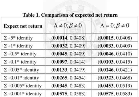
Table 1. Comparison of expected net return……..………...31

Table 2.Comparison of expected net return……..………...32

Table 3.Comparison of expected net return……..………...33

Table 4.Comparison of net return and the return per risk unit under 0 ; 0 ≠ ≠ Λ β ……..………...33

(7)

1 Introduction

1.1 Motivation and purpose

Today, in our society, accumulation of wealth could be a difficult task for most

people due to generally low salary structure, high commodity price, and low interest

rate. Hence, investment turns out to be one of the effective ways to solve this issue.

According to Brinson, Singer, and Beebower (1991), the main factors affecting

investment returns are asset allocation, entry timing, and stock picking, among which

asset allocation is the most influential one. In fact, the degree of influence of asset

allocation to the return of investment can be up to 91.5%. For economists or investors

who want to have satisfactory investment return figures, asset allocation is a very

important topic.

The main concept of traditional asset allocation is derived from the Mean-Variance

Portfolio Model published by Markowitz in 1952. This model deals mainly with the

asset allocation problem of a single period. However, today, in our modern society,

Markowitz’s model has become insufficient to cope with the rapidly changing

investment environment. In this paper, we first extend the Mean-Variance Portfolio

Model to two-period and then combine with other models to address the shortcoming of

the original model. Below is a brief introduction about the concept of the asset

allocation of single and multi-period. Asset allocation of single period, also known as

(8)

the traditional M-V model: No matter how the investment environment changes,

investors make investment decision only at the beginning of the period. Asset allocation

of multi-period: In several successive investment phases, investors will adjust the

allocation strategy according to the latest information after each period. The new and

much needed strategy is to readjust allocation weight in order to maximize the total

return of their investments or to minimize the overall risk of the investments.

Early discussion about asset allocation involved using past data as a basis for

future decision-making. However, Elam & Dixon (1988) pointed out that price series

data of the financial commodity are often non-stationary. The price showed random

walk, which means that price series of this period is not affected by that of the previous

period, so using past data to predict future price is not efficient. In addition, as

mentioned in the articles of Michaud (1989), Chopra & Ziemba (1993), Scherer (2002),

and Wolf (2006), estimation error of the mean, variance and covariance will have a

tremendous impact on the optimal portfolio. Therefore, information for future

decision-making is considered very important.

If a variable appears as a random walk type, then it is considered a non-stationary

variable. Granger and Newbold (1974) found that there would be spurious regression

phenomenon among non-stationary variables. Traditionally in the empirical research,

people mainly use regression methods to estimate the causal relationship between

(9)

variables. However, overlooking spurious regression might lead to the misinterpretation

of the result of empirical research. Hence, this fact that check whether variables are in

steady state cannot be ignored when time series variables are used for the study.

Therefore in this paper we check whether variables are in steady state first before we

use time series variables for the empirical study.

Later studies found that many time series of economic or financial variables have

non-stationary characteristic. Nelson and Plosser (1982) used a unit root test method to

study macroeconomic data collected in the U.S. and found that most of the

macroeconomic variables have the phenomenon of a unit root. In other words, most of

the economic variables follow non-stationary process. In tradition, people would

difference time series; however, important information might be lost as the result of

differencing the time series. Granger (1983) proposed the concept of cointegration

which uses cointegration vector to represent the relationship of the long-term mobile

trend between the non-stationary time series. When the data appears to be cointegrated,

it means that there is some information which may have a linear relationship. Thus the

data doesn’t need to go through the difference to be converted into stationary time series,

which solves the problem of information loss from differencing the time series. Engle

and Granger (1987) proposed the cointegration theory. According to their theory, if there

is cointegration phenomenon in the regression relationship between non-stationary

(10)

variables, then such a regression relationship still has economic significance.

Therefore, this paper uses the PCB Cointegration Model to organize the sequence

information of the price of financial commodity into the VAR (1) type. However, the

parameters in the formula VAR(1) must meet the formulas(4) (5) (6) in this paper.

Then we solve the problem of the future decision-making information with this model.

Traditionally, transaction cost is often overlooked in the discussion of asset

allocation. When examining multi-period asset allocation, one should worry about the

transaction cost becoming larger than the investment return due to frequent trading. In

fact, transaction cost is always imposed when trading financial products. In order to

model the common practice, transaction cost will be included in the following

discussion.

This paper uses the above model to compare the one-stage method with the

two-stage method: under the same risk, which method can bring a higher net return at

the end of the two periods. Net return is defined as the total return subtracting

transaction cost. With the one-stage method, the investment decision for both stages is

made at the beginning of the first stage based on the information available at time.

With the two-stage method, we make the investment decision for the first stage at the

beginning of the stage according to the information available at time; and when the first

(11)

phase is ended, we then use the new information available to make the best decision for

the second phase.

1.2 Framework

This article is divided into five chapters. A brief description of the content in each

chapter is as follows:

Chapter 1 Introduction

This chapter describes the motivation, purpose, and structure of the research in this

paper.

Chapter 2 The Cointegration Model

This chapter describes the cointegration model.

Chapter 3 Research Method

This paper uses formula(3) transformed from PCB Cointegration Model to

organize the sequence information of the price of the financial commodity, and then

uses the mean-variance optimization method to set the objective function for this paper.

We examine the one-stage method and the two-stage method of the dynamic portfolio

selection approach and determine which one can produce better net expected return

when undertaking the same risk.

Chapter 4 Numerical Illustrations

Among the 19 sector indices in the Taiwan market, we pick 5 that are I(1)

(12)

sequences then find their cointergration relationship. Next, estimate the model

parameters and use numerical methods to compare one-stage method and two-stage

method.

Chapter 5 Conclusions and Recommendations

We draw conclusions from the empirical results in chapter 4 and make

recommendations of future research on this topic.

(13)

Figure 1. Framework

Motivation and Purpose

The Cointegration Model

Research Method

One-stage method:

Complete the optimal asset allocation for both phases at the beginning of the first phase

based on the initial price.

Two-stage method:

Complete the optimal asset allocation for each phase at the

beginning of each phase based on prices at that time.

Discuss dynamic asset allocation using the mean-variance optimization method.

Comparison of Two Methods

Numerical Illustrations

Conclusions and Recommendations

Forecast asset price using PCB Cointegration Model.

,

, 2 1 , 2 2 , 2

, 1 , 2 1

, 1













+ +

=

+ Ξ +

=

− t

t t

t t T t

b x x

θ

θ t =1,2,...,n; ~ (0, )

, 2

,

1  Σ







= N b

b b

iid

t t t

(14)

2 The Cointegration Model

In this chapter, we will show Cointegration Model which will be used to organize

the sequence information of the price of the financial commodity in this paper.

Before being engaged in each type of statistical inference of the time series, we

should first examine whether the sequence is in stationary state. When the time series is

stationary, its data follows a stochastic process, but the probability distribution of this

stochastic process does not change along with time; otherwise, this time series is called

non-stationary time series.

Elam & Dixon (1988) pointed out that the price series of financial products usually

show the characteristic of non-stationary process. That means the price sequence is a

random walk type in which the price sequence of current period is not affected by the

price sequence of the previous period. If a time series is non-stationary, the commonly

used method to convert it to stationary is to take the difference on the variable or

eliminate the tendency item. However, the conversion could potentially eliminate the

implicit long-term message from the data, so to avoid this potential problem, we could

adopt the cointegration concept proposed by Granger. According to the cointegration

concept, a stable long-term balanced relation might exist between unstable variables,

and this relation might cause synchronized tendency on the variables. Therefore, we use

(15)

formula(3) transformed from PCB Cointegration Model to model price sequence of

finance commodity in this paper.

PCB Cointegration model

,

, 2 1 , 2 2 , 2

, 1 , 2 1

, 1













+ +

=

+ Ξ +

=

− t

t t

t t T t

b x

x

b x x

θ

θ t =1,2,...,n; ~ (0, )

, 2

,

1  Σ







= N

b b b

iid

t t

t (1)

First, move x₁_,_t、x₂_,_t to the left of formula(1) as below:













+ +

=

+

= Ξ

−

− t

t t

T t

b x

x

b x

x

, 2 1 , 2 2 , 2

, 1 1 , 2 ,

1

θ

θ (2)

Next, rewrite Eq.(2) in vector andmatrix forms.





 +













 +







=



















 −Ξ

−

t t

t t T

b b x

x x I

x I I

, 2

, 1

1 , 2

1 , 1

2 1

, 2

, 1

0 0 0

0 θ

θ



















 −Ξ

+



























 −Ξ

+



















 −Ξ

=







 ⁻

−

t t T

T

t t

b b I

I x

x I I

I I

I x

x

, 2

, 1 1

1 , 2

1 , 1 1

2 1 1

, 2

, 1

0 0 0 0 0

0 θ

θ



















 Ξ

+



























 Ξ

+



















 Ξ

=

−

t t T

T

b b I I x

x I I

I I

I

, 2

, 1

1 , 2

1 , 1

2 1

0 0 0 0 0

0 θ

θ

_t

t t T

x u x I +



















 Ξ

+

=

−

− 1 , 2

1 , 1

0

β 0

_t

t

t u

x x +





 Π +

=

−

− 1 , 2

1 ,

β 1 (3)

t t

t x u

x =β +Π ₋1 + , its form is similar to VAR(1). Its coefficient vector and matrix, β^&Π, and random vector, u , are as follows: _t





















 Ξ

=

2 1

0 θ

β θ

I I ^T

(4)

(16)











 Ξ

=

Π I

T

0

0 where the property of Π:

Π1 =Π−I; 



 



− Ξ

=

Π¹ 0 0 I T

; Π^k =Π, k =1,2,3...; Π₁Π=0⁽⁵⁾

~ (0, )

0 2,

,

1  Σ∗



















 Ξ

= N

b b I u I

iid

t t T

t where

T T T

I I I

I 









 Ξ

Σ











 Ξ

= Σ^∗

0

0 (6)

3 Research Method

3.1 Notations

x denotes the random vector of asset prices taken logarithm at time t. According to t

formula(3), x_t =β +Πx_t₋1+u_t^{. When}t≥², thex can be rewritten as: _t

( )

t

i i

t t x u u

x = + − Π +Π +Π

∑

⁻ +

= 1

1

1 β 0

β (7)

r ,t rt =xt −xt₋₁ , denotes the random vector of asset return during the time interval,

(

^t⁻¹^,^t

)

.According to formula(3):

t t t

t

t x x x u x x u

r = − ₋₁ =β+Π ₋₁+ − ₋₁ =β +Π₁ ₋₁+ (8) Whent≥2, thex can be rewritten as: _t

t t t

t

t x x u u

r = − ₋₁ =Πβ +Π₁ ₋₁ + (9) State : Eachx represents state t. _t

Stage : Stage t represents the range between x_t₋₁ and x . Stage is also called period. _t

w denotes the weight of asset allocation between t x_t₋₁ and x . This is the weight that _t we allocate at stage t. When we know the price of assetsx , we should know all the _t

weights that are less than or equal to that at staget+1. For example, when we

(17)

know the price of assetsx₁, we should know the price of assetsx , then we can ₀

know the weightsw₁andw₂. In addition, positive weight represents buying of

stocks; negative weight means selling or short selling of stocks. Prices of financial

products do not always go up; they may go down as well. Short selling is the

trading option to maximize profits during down time, thus we allow short selling in

this paper. Because our assumption allows short selling of stocks, the sum of the

weights in each stage does not need to be equal to one.

Λ denotes the fees charged for different trading methods, such as buying, selling, and

short selling of stocks. It is determined based on the weight. For the convenience of

problem solving and calculation, we represent it using a fixed ratio. And we assume

that Λis a symmetric positive definite matrix. The model of the transaction cost in

this paper is w^TΛw 2

1 . The reason we use quadratic form to present the model of

transaction costs in this paper is to avoid the transaction costs becoming negative.

Because we allow negative weight, we must use the quadratic form to ensure that

transaction cost is positive.

Since we apply two-period dynamic asset allocation, the maximum number of t =2.

3.2 Objective functions

Markowitz's mean-variance portfolio optimization methods provide two

approaches: (1) under fixed risk, find the maximum return or (2) under fixed

(18)

remuneration, minimize the risk. The method that we chose in this paper is the former,

which is to find maximum return under fixed risk. In the special case of the following

section, we will verify that both methods give the same return when undertaking a unit

risk.

This paper uses two-stage mean-variance portfolio optimization framework, and

the objective function is as follows:

( )

1 1 2 2 0 1 1

(

2 1

) (

2 1

)

0

2 ,

1 2

max 1 ,

2 1

x w w w

w w w E x

r w r w E w

w

f ^T ^T ^T ^T

w

C = w + − Λ + − Λ − (10)

Restriction is as follow:

Var w¹^Tr¹+w²^Tr² x⁰ =σ⁰²

That means we want to optimize the net expected return of two-period, which is

deducting transaction cost under the constraint of restricting the variance of total return

toσ₀²at the end.

The objective function (10) and its restriction in this case which use the Lagrange

multipliers method can be rewritten as:

( )

1 1 2 2 0 1 1

(

2 1

) (

2 1

)

0

2 ,

1 2

max 1 ,

2 1

x w w w

w w w E x

r w r w E w

w

f ^T ^T ^T ^T

w

C = w + − Λ + − Λ −

[

¹ ¹ ² ² ⁰ ⁰²

]

2 σ

λ ₊ ₋

− ^C Var w^Tr w^Tr x (11)

where λ_C is a Lagrange multiplier.

Below we will discuss one-stage method and two-stage method respectively.

(19)

3.3 Dynamic portfolio selection methods

3.3.1 One-stage method

At statex , we optimize asset allocation for two periods according to asset prices ₀

at statex .₀

First, the objective function sort out from (11) is as follow:

( )

^w ⁼^E ^w ^r ^x⁰ ⁻¹₂^w ^Λ^∗^w⁻

^λ

₂¹

[

^Var ^w ^r ^x⁰ ⁻

^σ

⁰²

]

f_CO ^T ^T ^T

[

⁰ ⁰²

]

1

0 2 2

1 _Λ ₋

λ

₋

σ

−

=w^TE r x w^T ^∗w w^TVar r x w

[

⁰²

]

1

2 2

1 _Λ ₋

λ

₋

σ

−

=w^TA w^T ^∗w w^TBw

(12) The vectors andmatrices represent respectively:





 



=

2 1

w

w w ； 



 



=

2 1

r

r r ； 



 





Λ Λ

−

Λ

−

= Λ Λ^∗ 2

；









=

=

0 2

0 1

0 E r x

x r x E

r E

A ；







=

=

0 2 0

1 2

0 2 1 0

1

0 ,

, x r Var x

r r Cov

x r r Cov x

r x Var

r Var B

Then to optimize the objective function, we perform the first order differential equal to

zero on it.

1 =0

− Λ

− ^∗w Bw

A λ

w_CO =Ψ⁻¹A where ^Ψ ⁼

(

^Λ^∗ ⁺^λ¹^B

)

(13)

(20)

According to 3.1 (8)、(9), the results are derived as follows:

0 1 0

1 0 1 0

1 x E x u x x

r

E = β +Π + =β +Π β

β+Π + =Π Π

= 1 1 2 0

0

2 x E u u x

r

E Σ∗

= +

Π +

= 1 0 1 0

0

1 x Var x u x

r

Var β

D x u u Var

x r

Var 2 0 = Πβ +Π1 1 + 2 0 = ^where D=Π₁Σ^∗Π₁^T +Σ^∗

0 2 1 1 1

0 1 0

2

1,r x Cov x u , u u x

r

Cov = β +Π + Πβ +Π +

x T

u u

Cov ₁,Π₁ ₁ ₀ =Σ Π₁

= ^∗

Since weight w_CO(13) contains an unknown figure λ₁, we try to use the equation of

constraint to solve λ₁. In fact, in the process of finding solution, we will see λ₁^{in the}

anti-function, and there is no way to find solution from that function directly.

Therefore, our approach is to get a starting estimate λ₁^∗ by using Taylor expansion first.

(The detailed derivations are in Appendix1.1.1.)

A B

B A

A B

A

T T

⋅ Λ

⋅

⋅ Λ

⋅

⋅ Λ

⋅

−

⋅ Λ

⋅

⋅ Λ

≈ ⋅ ₋

− ∗

∗

∗−

∗

1 1

1

2 0 1

1

1 2

λ σ (14)

Then from the formulaVar w_CO^T r x₀ =σ_O², we can sort out an identity equation.

2 0 1 1

1

1⋅ − ⋅Ψ ⋅Λ ⋅Ψ ⋅ =λ ⋅σ

Ψ

⋅ ⁻ A A ⁻ ^∗ ⁻ A

A^T ^T (15)

Next, we take the initial estimated value λ^∗₁ into the function Ψ⁻¹of the left side of Eq.

(15), and then we can get a new estimated value from the right side of the equation. We

(21)

then confirm if the difference between the initial estimated value and the new estimated

value is less than the estimated error of our setting. If not, we take the new estimated

value and substitute it into the left side of the formula until the values of two sides are

very close, expressing convergence, then we stop. If so, we can get an answer directly,

which results in a more accurate estimated valueλ₁^S^.

The optimal weight of one stage method:

w_CO^∗ =Ψ^∗⁻¹A where ^Ψ^∗ ⁼

(

^Λ^∗ ⁺^λ¹^S^B

)

(16) Expected return after deducting transaction cost of one-stage method as follows:

^∗ − ^∗ Λ^∗ ^∗ = ^∗ − ^∗ Λ^∗ ^∗CO

T CO T

CO CO T CO T

CO r x w w w A w w

w

E 2

1 2

1

0

= A^T ⋅Ψ^∗⁻¹⋅A− A^T ⋅Ψ^∗⁻¹⋅Λ^∗⋅Ψ^∗⁻¹⋅A 2

1

⁼ ^A^T ^⋅^Ψ^∗⁻¹^⋅^A⁻₂¹

(

^A^T ^⋅^Ψ^∗⁻¹^⋅^A⁻^λ¹^S ^⋅^σ⁰²

)

⁼ ¹₂

(

^A^T ^⋅^Ψ^∗⁻¹^⋅^A⁺^λ¹^S ^⋅^σ⁰²

)

3.3.2 Two-stage method

At beginning of the first period, we will allocate the weight of asset based on the

initial price. We will then re-allocate the weight of asset again based on the asset price at

beginning of the second period.

In this method, we use the backward way to solve it. In other words, we get the

optimal weight of the second phase by using the objective function of the second phase.

(22)

Then we apply the optimal weight of the second stage to the overall objective function

to get the optimal weight of the first phase.

In this paper, we don’t consider the transaction cost in the objective function of the

second stage. Instead, we use an undetermined coefficient a₁ to adjust the change.

Step1.

Supposex and₀ x₁are known, the objective function of the second phase is as follow:

( )

² ² ² ⁰ ¹ ² ² ⁰ ¹

2 ,

2

,x 1Var w r x x x

r w E w

f = ^T − ^T

2 1 0 2 2 1

0 2

2 ,

2

,x 1w Var r x x w x

r E

w^T − ^T

=

We want to obtain the optimal decision of the second stage, so we perform the first

order differential equal to zero on it.

0 ,

, ₁ ₂ ₀ ₁ ₂

0

2 x x −Var r x x w =

r E

( )

2 0 1

1 1 0 2

*

2 Var r x ,x E r x ,x

w = ⁻

According to 3.1 (8)、(9), the results are derived as follows:

1 1 1

0 2 1 1 1

0

2 , ,

r x x E x u x x x

E = β +Π + =β +Π Σ∗

= +

Π +

= 1 1 2 0 1

1 0

2 , ,

r x x Var x u x x

Var β

The deduced result is obtained:

1

*

2 x

w =γ +Φ where ^γ ⁼

( )

^Σ^∗ ⁻¹^β ^；^Φ⁼

( )

^Σ^∗ ⁻¹^Π¹

We apply factor a₁ then it becomes:

(

1

)

1

* 2

1w a x

a = γ +Φ (17)

(23)

Step2.

Next, we must take the optimal weight of the second phase (17), which multiplies

an undetermined coefficienta₁, to substitute it into the optimal objective function of two

periods (11), as shown below:

(

¹ ¹

)

¹ ¹ ¹ ² ² ⁰ ¹ ¹

(

¹ ² ¹

) (

¹ ² ¹

)

⁰

2

,a E w r a w r x 1E w w a w w a w w x w

f_CT = ^T + ^∗^T − ^TΛ + ^∗− ^TΛ ^∗ −



 + −

− ² ₁ ₁ ₁ ₂^∗ ₂ ₀ ₀²

2 σ

λ Var w^Tr aw^Tr x

The objective function is sorted out as following:

( )

^V ⁼^E ^V ^Z ^x⁰ ⁻₂¹^E ^V ^CV ^x⁰ ⁻^λ₂²

[

^Var ^V ^Z ^x⁰ ⁻^σ⁰²

]

f_CT ^T ^T ^T

⁰ ⁰ ²

[

⁰ ⁰²

]

2 2

1 ₋λ ₋σ

−

=V^TE Z x V^TE C x V V^TVar Z x V ²

[

⁰²

]

2 2

1 ₋λ ₋σ

−

=V^TF V^THV V^TGV (18)

The vectors andmatrices represent respectively:



 



=

1 1

a

V w ； 



 



= _∗

2 2

1

r w

Z rT ； 



 





Λ Λ

−

Λ

−

= Λ_∗ _∗ ^∗_∗

2 2 2

2 2

w w w

C _T _T w ；











=

= _∗

0 2 2

0 1

0 E w r x

x r E x

Z E

F ^T ；













Λ Λ

−

Λ

−

= Λ

= _∗ _∗ _∗

∗

0 2 2 0

2

0 2 0

0

2

x w w E x w E

x w E x

E x

C E

H T T ;

















=

= ∗

0 2 2 0

1 2

* 2

0 2

* 2 1 0

1 0

,

, x r w Var x

r r w Cov

x r w r Cov x

r Var x

Z Var

G _T _T

T

After the first order differential, we get:

2 =0

−

−HV GV

F λ

(24)

F

V^∗ =Ω⁻¹ where ^Ω⁼

(

^H ⁺^λ²^G

)

(19) According to 3.1 (8)、(9), the results are derived as follows:

(

1 0 1

)

1 0

0

1 x E x u x

r

E = β +Π + =β +Π

=l

0 2

*

2 r x

w

E ^T where l=^L^TΠβ +^tr

( )

ϕ ; L=

(

γ +Φβ

)

; =Φ Π1Σ^∗

ϕ T

Σ∗

= +

Π +

= 1 0 1 0

0

1 x Var x u x

r

Var β

k x r w

Var ^T 2 0 =

*

2 where D=Π₁Σ^∗Π₁^T +Σ^∗； =Φ Π1Σ^∗

ϕ T

(

^γ

)

^β

( )

^ϕ

( )

^ϕ

(

^β

)

^β

γ

γ + + Φ + + + Π Φ+ Π Σ Φ Π

= 1 ^∗ ^T

2

T 2 ^T ^T 2 ^T

T

TD L D tr tr L

k

N x r w r

Cov ^T 2 0 =

* 2

1, where ^N ⁼^Σ^∗

(

^Π¹^T^γ ⁺^Π¹^T^Φ^β ⁺^Φ^T^Π^β

)

Λ

=

Λ 2

2 x₀

E

L x

w

E Λ 2^∗ 0 =Λ where L=

(

γ +Φβ

)

( )

1 0

2

2 ^w ^x ^L ^L ^trϕ

w

E ^∗^TΛ ^∗ = ^TΛ + where L=

(

γ +Φβ

)

； ϕ1 =Φ^TΛΦΣ^∗

Same as one-stage method, the vector V^∗of two-stage method also contains unknown figureλ₂ and there is no way to utilize equation of constraint to solveλ₂. Hence, we

also get a starting estimateλ^∗₂ by Taylor expansion.

F H G H G H F

F H G H F

T T

⋅

−

⋅

≈ ⋅ ₋⁻ ₋⁻ ₋

∗

1 1

1

2 0 1

1

2 2

λ σ (20)

Then from the formulaVar V^∗^TZ x₀ =σ₀², we can sort out an identity equation.

(25)

2 0 2 1

1

1⋅ − ⋅Ω ⋅ ⋅Ω ⋅ =λ ⋅σ

Ω

⋅ ⁻ F F ⁻ H ⁻ F

F^T ^T (21)

Next, we take the initial estimated value λ^∗₂ into the function Ω⁻¹of the left side of

Eq.(21), so that we can get a new estimated value of the right side of the equation. We

then confirm if the difference of the initial estimated valueλ^∗₂and the new estimated

value is less than the estimated error of our setting. If not, we take the new estimated

value and substitute it into the left side of the formula until the value of two sides are

very close, expressing convergence, then we stop; If so, we can get an answer directly,

which would result in a more accurate estimated valueλ^S₂^.

The two-stage method obtains a vectorV_λ^∗which is combination of the optimal weight of

the first stage and a scale factor. V_λ^∗ =Ω^∗⁻¹F where ^Ω^∗ ⁼

(

^H⁺^λ^S²^G

)

(22) Expected return of two-stage method minus transition cost is represented as follows:

0

0 2

1E V CV x

x Z V

E _λ^∗^T − _λ^∗^T _λ^∗

∗

∗ −

=V_λ^TF V_λ^THV_λ 2

1

= F^T ⋅Ω^∗⁻¹⋅F − F^T ⋅Ω^∗⁻¹⋅H⋅Ω^∗⁻¹⋅F 2

1

⁼ ^F^T ^⋅^Ω^∗⁻¹^⋅^F ⁻¹₂

(

^F^T ^⋅^Ω^∗⁻¹^⋅^H ⁻^λ²^S ^⋅^σ⁰²

)

⁼ ¹₂

(

^F^T ^⋅^Ω^∗⁻¹^⋅^F ⁺^λ²^S ^⋅^σ⁰²

)

(26)

3.4 Special Cases

In this section, we will show four special cases.

Case #1: The first example is the typical Markowitz mean-variance portfolio

optimization approach in which asset allocation decisions are made at the beginning of

the investment period according to the price at the time regardless of the length of the

investment period. In other words, the asset allocation weight will not be changed

through time. This method is also known as static method. In this paper, we will

transform the PCB Cointegration Model to formula(3), and then incorporate the new

model together with the transaction cost model into the static method.

The objective function of the static method is as follows:

^f^C

( )

^w ⁼^max_w ^E ^w^T^r ^x⁰ ⁻¹₂^w^T^Λ^w⁻

^λ

₂

[

^Var ^w^T^r ^x⁰ ⁻

^σ

⁰²

]

[

⁰²

]

2 2

1 _Λ ₋λ ₋σ

−

=w^TA_S w^T w w^TB_Sw

According to the definition of return in 3.1 (8)、(9), the return random vector is as

follows:

(

2 1

) (

1 0

)

2 1 1 1 2 1 0 1

0

2 x x x x x r r u u x u

x

r = − = − + − = + =Πβ+Π + +β +Π +

=Π1x0 +

(

Π+I

) (

β + Π1+I

)

u1+u2 =Π1x0 +

(

Π+I

)

β+Πu1+u2 (23) After taking the first order differential, we get:

S

S A

w =Μ⁻¹ where Μ =

(

Λ+λBS

)

(24)

(27)

Result derived according to Eq.(23) is as follows:

(

^I

)

β ^u ^u ^x ^x

(

^I

)

β

x E x r

E 0 = Π1 0 + Π+ +Π 1 + 2 0 =Π1 0 + Π+

Var r x0 =Var Π1x0 +

(

Π+I

)

β +Πu1+u2 x0 =ΠΣ^∗Π^T +Σ^∗ Then, with the same approach used previously to estimate valueλ, we get a more

accurate estimateλ_S, thus the expected return after deducting transaction cost of static

method is as follows:

^E ^w^∗^S^T^r ^x⁰ ⁻¹₂^w^∗^S^T^Λ^w^S^∗ ⁼¹₂

(

^A^S^T ^⋅^Μ^∗⁻¹^⋅^A^S ⁺^λ^S ^⋅^σ⁰²

)

Case #2: Given the conditionΛ≠0;β =0, compare the two dynamic methods to

determine which method gives higher expected return after deducting transaction cost.

(See Appendix 1.2、2.2 for the detailed derivations)

The objective function is as follows:

( )

1 1 2 2 0 1 1

(

2 1

) (

2 1

)

0

2 ,

1 2

max 1 ,

2 1

x w w w

w w w E x

r w r w E w

w

f ^T ^T ^T ^T

w

C = w + − Λ + − Λ −

⁻^λ₂^C

[

^Var ^w¹^T^r¹⁺^w²^T^r² ^x⁰ ⁻^σ⁰²

]

Expected return after deducting transaction cost of one-stage method is as follows:

^E ^w^∗^CO^T^r ^x⁰ ⁻¹₂^w^CO^∗ ^T^Λ^∗^w^CO^∗ ⁼ ₂¹

(

^A⁰^T ^⋅^Ψ^∗⁻¹^⋅^A⁰ ⁺^λ³^S ^⋅^σ⁰²

)

Expected return after deducting transaction cost of two-stage method is as follows:

^E ^V^λ^∗^T^Z ^x⁰ ⁻₂¹^E ^V^λ^∗^T^CV^λ^∗ ^x⁰ ⁼ ¹₂

(

^F⁰^T ^⋅^Ω⁰^∗⁻¹^⋅^F⁰^T ⁺^λ⁴^S ^⋅^σ⁰²