國立臺灣大學電機資訊學院電信工程研究所 碩士論文
Graduate Institute of Communication Engineering College of Electrical Engineering and Computer Science
National Taiwan University Master Thesis
廣義分頻多工系統中頻寬效率最大化之原型濾波器設計 Prototype Filter Designs for Maximizing Spectral
Efficiency in Generalized Frequency Division Multiplexing Systems
貝律祥 Lucien Bernard
指導教授:蘇柏青 博士 Advisor: Borching Su, Ph.D.
中華民國 107 年 7 月 July, 2018
Acknowledgements/誌謝
I am now able to complete my master’s thesis, and I must politely thank the many people who contributed to the exercise, and finally the accomplish- ment of the work required by the dual degree program for which I was enrolled for this academic year.
Firstly, I pay particular attention to the dedication and patience shown by my master’s advisor, Professor 蘇柏青, who produces a very hard work at the lowest estimate, in order to develop the autonomy of his students in terms of individual productivity, through weekly meetings, and encouraging group work through the connection of projects to common bases. Thanks to my previous experience of project autonomy in the field of microwaves as part of my engineering studies in France, I was led to work on a problem already developed by several colleagues in the laboratory; precisely, the candidate waveforms of the next-generation communication systems, in order to solve a new problem of convex optimization, which turns out to be the teaching speciality of Professor 蘇. Through this process, I solved a problem of max- imization of subcarriers and subsymbols, which constitutes the major part of this master’s thesis.
Secondly, I would like to thank 黃彥銘 for allowing me to have a different approach to understanding the master’s thesis on which I base my research.
This valuable assistance became my initial motive for the whole document
and yielded fruitful results. At the same time, I would like to thank 林 政 諺 for the many valuable opinions and suggestions it provided me during my research. Thanks also to the laboratory colleagues 許家霖, 賈才 and 邱浩則 who honestly and sincerely contributed well to technical support and mutual aid during this academic year. Moreover, thanks to the tolerance and support of my family, I can concentrate on my research and carry out this thesis.
Finally, I thank once again Professor 蘇 柏 青 for his many suggestions and encouragement, so that I can successfully edit a master’s thesis marking the completion of one of my engineering trainings. I acquired a lot of pro- fessional knowledge and research methods from Professor 蘇. I express my deep gratitude here.
v
Abstract
Generalized frequency division multiplexing (GFDM) is a recent block filtered multicarrier modulation scheme featuring low out-of-band (OOB) ra- diation and low latency. By using a matrix-based characterization of GFDM transmitter matrices, opposed to traditional vector-based characterization with prototype filters, and deriving properties of GFDM (transmitter) matrices, one can design prototype filters that are found to correspond to the use of unitary GFDM matrices many scenarios, while avoiding the problem of noise en- hancement, thereby showing the same MSE performance as orthogonal fre- quency division multiplexing (OFDM).
In this thesis, a new problem related to bandwidth efficiency, and espe- cially for OOB part, has been formulated in order to manage and design the number of used subcarriers and used subsymbols, so that the spectral effi- ciency can be maximized, regarding specifications needed by the prototype filters designers. A previous work introducing a filter optimization algorithm, originally introduced as a non-convex problem, tackled to an algorithm of two convex problems, that minimizes OOB radiation while maintaining good in- band performance is developed for GFDM is used in order to solve this prob- lem, knowing that the spectral efficiency will be a main constraint.
Since the main problem is about a maximization of sets of used subcarriers and used subsymbols, the resolution technique is however not well developed
in the literature, while it is a known encountered problem. From that point on, the thesis proposes three methods to address this problem. The first intro- duces a raw force calculation, improved by a stopping criterion, knowing the non-decreasing nature of the function put into play under constraint. The two others methods propose an advanced algorithmic calculation in order to speed up the resolution of the maximization problem, by comparing the values al- ready calculated, and knowing before the next calculation, which solution can potentially be better. The different simulations results show that the designer can choose a method and this number of subcarriers and subsymbols so that to treat the number of users, for the proper utilization of this characteristic GFDM system.
Keywords: Generalized frequency division multiplexing (GFDM); charac- teristic matrix; optimal prototype filters; out-of-band (OOB) radiation; spec- tral efficiency; parameter design; performance constraints
vii
Contents
口試委員會審定書 ii
Acknowledgements/誌謝 iv
Abstract vi
1 Introduction 1
2 Characterization of GFDM Systems & Problem Statement 5
2.1 Related work to matrix characterization for GFDM systems . . . 5
2.1.1 Characterization of GFDM Matrices: Basic Definition . . . 6
2.1.2 Unitary and Invertible GFDM Matrices . . . 7
2.1.3 GFDM Transmitter Implementations . . . 8
2.2 Definition of Prototype Filters for Maximizing Spectral Efficiency . . . . 10
2.2.1 Optimization Problem maximizing the spectral efficiency . . . . 10
2.2.2 Problem formulation . . . 11
3 Proposed methods 13 3.1 Method 1: complete calculation by raw force . . . 14
3.2 Method 2: 2D to 1D matrix reshaping . . . 16
3.3 Method 3: 2D matrix calculation . . . 19
3.3.1 Comparison between Method 3.2 and Method 3.3 . . . 21
4 Results and discussion 23 4.1 Simulation results . . . 24
4.1.1 Method 3.1: complete calculation by raw force . . . 24
4.1.2 Method 3.2: 2D to 1D matrix reshaping and Method 3.3: 2D ma- trix calculation . . . 26
4.2 Limits of the methods and discussion . . . 29
5 Conclusion 31 Bibliography 33 Power Spectral Density and OOB Leakage 35 Used algorithm 39 Proof of non-convexity for (B.2d) 43 Add-ons about about g settlement and PSD calculation 45 .1 Proof of discrete-time Fourier transform of gm[n] . . . . 45
.1.1 No cyclic prefix (L=0) . . . . 45
.1.2 With cyclic prefix (L=0) . . . . 47
.2 Rewriting Sa(f ) . . . . 48
ix
List of Figures
2.1 Block diagram of the transceiver. . . 6 3.1 Sequential flowchart of the proposed method . . . 20
Chapter 1 Introduction
Generalized frequency division multiplexing (GFDM) [1], extensively studied in recent years, is a potential modulation scheme for incoming wireless communication systems, particularly in the Internet of things (IoT), because it features good properties including low out-of-band (OOB) radiation and flexible time-frequency structures to adapt to var- ious application scenarios, such as cognitive radios and low latency applications [2]. A recent work [3] proposed a matrix characterization for GFDM systems. Specifically, it introduced low complexity minimum mean-square error (MMSE) receivers and optimal filters. In order to continue in this particular settlement, a filter optimization of OOB radiation with performance constraints for GFDM systems has been studied [4]. An opti- mization problem has been formulated, along with descriptions of the characteristic matrix and closed-form expressions for the noise enhancement factor (NEF) and power spectral density (PSD) of GFDM signals.
However, although this previous work studied the feasibility of low-complexity MMSE receivers in presence of multipath channels and propose the first implementation with lin- earithmic complexity, it thus does not provide a preliminary research of design the number and position of guard subcarriers and subsymbols. The prototype filters already used in different studies involving GFDM choose these parameters in an undefined way, or even in an arbitrary manner. Beside this, it is still unclear in the literature to find explanations about a good management of those paramaters. That is why we want to arise this question
in this thesis.
In addition, given that the optimization problem is formulated in terms of the proposed characteristic matrix of the GFDM transmitter matrix, results of the previous work [4] have shown that under the same spectral efficiency, optimized filters perform the best in terms of both OOB radiation and symbol error rate (SER) performance, compared to RC filters, Dirichlet pulses, and OFDM. Finally, the advantage of GFDMA using CMCM filters, including the Dirichlet and modified Dirichlet pulses, over OFDMA has been verified through numerical results. In this thesis, we manage some suggestions to design those prototype filters [4], based on the previously introduced characteristic matrix, in order to design the number and position of guard subcarriers and subsymbols, while maximizing spectral efficiency under OOB radiation and keeping performance constraints.
This thesis thus offers one main contribution. Under prototype transmit filters in re- ceiver mean square error (MSE), we investigate the utilization of the previous matrix char- acterization [3], to introduce two methods of calculation, in the idea of minimizing the number of calculation steps necessary to quickly and efficiently calculate the number of subcarriers and subsymbols satisfying an optimization problem. This non-convex opti- mization problem proposes to maximize the product of those numbers of subcarriers and subsymbols. Then, thanks to the potential multiple results that could lead to the same result given by this product, we show how it is possible to determine certainly the exact number of subcarriers, and the exact one about subsymbols. This has to be shown, since one of the constraints introduced in the optimization problem, is to keep the maximum spectral efficiency under a limit fixed by the designer.
The remainder of this thesis is structured as follows. In Chapter 2, we present the GFDM system model and a previous consistent research. We also remind some deriva- tions of properties of GFDM matrices and present low-complexity transmitter implemen- tations, to finally the maximization problem. In Chapter 3, we plan to emphasize the
2
proposed methods to solve the problem introduced in the preceding chapter. In Chapter 4, simulation results about the problem are shown and discussed. Finally, the study con- clusion is provided in Chapter 7.
Notations: Boldfaced capital letters denote matrices, and boldfaced lowercase letters are reserved for column vectors. We use⟨·⟩D, (·)∗, (·)T, and (·)H to denote modulo D, complex conjugate, transpose, and Hermitian transpose, respectively. We also use (·)−H to denote(
(·)−1)H
. Given a matrix A, we denote by [A]m,n, [A]:,r, ∥A∥F, vec(A), tr(A), rank(A), and A−1its (m, n)-th entry (zero-based indexing), r-th column, Frobenius norm, column-wise vectorization, trace, rank, and Hadamard inverse (defined by[
A−1]
m,n = [A]−1m,n, ∀ m, n), respectively. For any diagonal matrix A, [A]n denotes [A]n,n. For any matrices A and B, A⊗ B denotes their Kronecker product, and A ◦ B their Hadamard product. Given a vector u, we use [u]n to denote the n-th component of u,∥u∥ the L2- norm of u, diag(u) the diagonal matrix containing u on its diagonal, and Ψ(u) the circulant matrix whose first column is u. We define Ip to be the p× p identity matrix, 1pthe p× 1 vector of ones, Wp the normalized p-point DFT matrix with [Wp]m,n = e−j2πmn/p/√p for any positive integer p, and δklthe Kronecker delta. We use E{·} to denote the expectation operator. Finally, we useH+D to denote the set of Hermitian positive semidefinite D× D matrices, and⪯ to denote the matrix inequality.
Chapter 2
Characterization of GFDM Systems &
Problem Statement
2.1 Related work to matrix characterization for GFDM systems
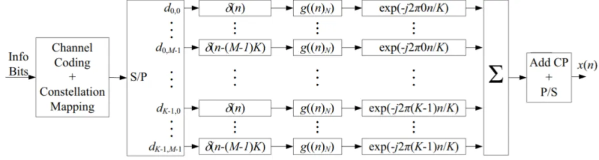
GFDM is a block-based communication scheme as shown in Figure 2.1 [2], which are proposed to satisfy the requirements of 5G. In this section, we summarize some important results of a previous work that we will use in this thesis to build up further investigations.
In a GFDM block, M complex-valued subsymbols are transmitted on each of the K sub- carriers, so a total of D = KM data symbols are transmitted. The data symbol vector d[l]
is decomposed as
d[l] = [d0,0[l]· · · dK−1,0[l] d0,1[l]· · · dK−1,1[l]· · · dK−1,M−1[l]]T ,
where dk,m[l] is the data symbol on the k-th subcarrier and m-th subsymbol in the l-th block, taken from a complex settlement. Therefore, it is possible to engineer the spectrum regarding given requirements and enabling pulse shaping on a subcarrier basis. By con- sidering that the data symbols are zero-mean and independent and identically distributed (i.i.d.) with symbol energy ES, id est, E{d[l]dH[n]} = ESIDδln. Each data symbol dk,m[l]
is thus transmitted via a pulse-shaped filter by the vector gk,mwhose n-th entry is a circu- larly shifted version of gk,0, and the complex exponential designates the shifting operation in the frequency domain :
[gk,m]
n = [g]⟨n−mK⟩
Dej2πkn/K, n = 0, 1,· · · , D − 1 (2.1)
where g is a D× 1 vector, referred to as the prototype transmit filter [2]. Let x[l] = [x0[l] x1[l]· · · xD−1[l]]T be the vector containing the transmit samples. They are under- stood as the superposition of all transmit symbols. Then, the GFDM modulator can be formulated as the transmitter matrix [2]
A =[
g0,0· · · gK−1,0g0,1· · · gK−1,1· · · gK−1,M−1
] (2.2)
such that x[l] = Ad[l]. The matrix A as defined in (2.2) is called hereafter a GFDM matrix with a prototype filter g. The vector x[l] is further added a cyclic prefix (CP) before sending to the receiver through a linerar time-invariant (LTI) channel. The complexity of
Figure 2.1: Block diagram of the transceiver.
this form is in O(KM log KM ). Yet, it has been shown in [3] that this implementation is advantageous for receiver implementation.
2.1.1 Characterization of GFDM Matrices: Basic Definition
In the literature, GFDM transmitter matrices are often characterized by a prototype trans- mit filter g. We will mainly use this notation in order to continue our study.
6
In this thesis, we use another means for characterizing a GFDM transmitter matrix, namely, the characteristic matrix G of size K× M. A formal definition of this character- ization of a GFDM transmitter matrix necessary for the understanding and continuation of the study, is given as follows.
Definition (Characteristic matrix) Consider a KM × KM GFDM matrix A in (2.2) with a prototype filter g. We define the characteristic matrix G of the GFDM matrix A as
G =√
D reshape(g, K, M )WM (2.3)
where reshape(g,K,M) is a K× M matrix whose (k,m)-entry is [g]k+mK, ∀ 0 ≤ k < K, 0 ≤ m < M. The reshape process needs to be used many times, especially for the de- velopment of our future methods. Since we will limit our study to a 2 dimensional matrix, we simply explain that the processus of reshaping proposes to rearrange the order of the elements of an initial matrix, under new conditions of size, so that the number of elements is still kept.
2.1.2 Unitary and Invertible GFDM Matrices
With the characteristic-matrix-domain implementation, we can also easily identify the class of unitary GFDM matrices as follows.
Theorem 1 (Unitary GFDM matrices) Let A be a GFDM matrix with a K× M char- acteristic matrix G. Then, A is unitary if and only if G contains unit-magnitude entries:
|[G]k,l| = 1 ∀ 0 ≤ k < K, 0 ≤ l < M.
The following theorem introduced in [3] is needed to express the conditions for the non-singularity of a GFDM matrix in terms of its characteristic matrix and related prop- erties.
Theorem 2 (Properties of A−1) Let A be a GFDM with a K× M characteristic matrix G. Then,
a A is invertible if and only if G has no zero entries ;
b if A is invertible, then A−H is also a GFDM matrix whose characteristic matrix H satisfies [H]k,l = 1/[G]∗k,l,∀ k, l, id est,
H = (G∗)◦−1 ; (2.4)
c if A is invertible, the squared norm of each row of A−1 equals the energy of A−H, ξH =∥H∥2F/D.
Note: a proof of this theorem is proposed in [3].
2.1.3 GFDM Transmitter Implementations
The transmitter simply modulates the data symbol vector by
x[l] = Ad[l]. (2.5)
Then, x[l] is passed through a parallel-to-serial (P/S) converter, and a CP of length L is added, as shown in 2.1. DenoteK ⊆ {0, 1, · · · , K − 1} and M ⊆ {0, 1, · · · , M − 1}
as the set of used subcarriers and set of used subsymbols respectively, that are actually enrolled.
The digital baseband transmit signal of GFDM is expressed as
x[n] =
∑∞ l=−∞
∑
k∈K
∑
m∈M
dk,m[l]gm[n− lD′]ej2πk(n−lD′)K , (2.6)
8
where D′ = D + L and
gm[n] =
[g]⟨n−mK−L⟩
D, n = 0, 1 . . . , D′− 1 0, otherwise
(2.7)
which is finally the transmitted part as shown in Figure 2.1.
Because GFDM is confined in a block structure of D samples, with K subcarriers car- rying M subsymbols each, it is possible to design the time-frequency structure to match the time constraints of low latency applications. Different filter impulse responses can be used to filter the subcarriers and this choice affects the OOB emissions and the SER performance. However, a simple example of M-ary Frequency Shift Keying (MFSK) has shown [5] that increasing the number of symbols leads to a poor spectral efficiency. Spec- tral efficiency means to utilize the available spectrum as efficient as possible. One could say that maximizing the spectral efficiency should base on the channel gains of the users.
It is also known that using by convention guard subcarriers or subsymbols for engineer- ing is still affordable and understandable, since it generally stems from a inter-symbol interference. Instead of just dividing the spectrum into subcarrier and separating them by introducing guard bands these carriers overlap but are orthogonal due to the nature of the pulse shaping.
As a reminder, we denoteK ⊆ {0, 1, · · · , K − 1} and M ⊆ {0, 1, · · · , M − 1} as the set of used subcarriers and set of used subsymbols. In [4], K has been selected as an odd number for each case because RC filters are essentially not applicable to cases where both K and M are even, as GFDM transmitter matrices under such cases are singular. By computing the method in [4], we can also notice that setting different couples (|K|; |M|) give a better spectral efficiency for a same result of a product of these parameters. Since it is still unclear to obtain a true determination of a design for the utilization of involved subcarriers for the setK and involved subsymbols for the set M in a GFDM system, this raises a main consequent problem, that is to say how to settle and designK and M so that
we can maximize the number of users through maximizing the spectral efficiency.
2.2 Definition of Prototype Filters for Maximizing Spec- tral Efficiency
In this section, we use the design of previous prototype filters [4] considering performance and OOB radiation simultaneously.
The following lemma would be useful for derivations of low-complexity transceiver implementations and optimal prototype filters later, whose proofs can be consulted in [3].
Lemma Let A be a GFDM matrix with a K × M characteristic matrix G, a D × 1 prototype filter g, and energy ξG, where D = KM . Then, the prototype filter g can be expressed as g = vec(
GWHM) /√
D.
2.2.1 Optimization Problem maximizing the spectral efficiency
In order to design our prototype filters, we need to include a filter optimization problem minimizing OOB radiation while maintaining good in-band performance, introduced in [4]. By considering a GFDM system with the GFDM transmitter matrix A and prototype filter g, let K, M , L,K, ES, Ts, p(t) andBO denoting the set of frequencies considered out of band. LetM = {1, 2, · · · , M − 1}, id est, one guard subsymbol is used, which is conventional in the literature [6]. Let D = KM and η be some positive real number. The optimization problem is given by
minimize
g max
f∈BO
Sa(f ) (2.8a)
subject to ∥g∥2F = 1, (2.8b)
ξH ≤ η, (2.8c)
where Sa(f ) is the PSD (see 5) of the GFDM analog baseband transmit signal, and ξH is the energy of A−1. Actually, ξH determines the signal-to-noise ratio (SNR) reduction of
10
a GFDM system. The constraint (2.8c) pertains to maintain a sufficiently good MSE or SER performance. The constraint (2.8b) is set as the normalization the prototype filter g.
Besides, according to (2.3) and the definition of energy of a GFDM matrix, the constraint (2.8b) implies a natural constraint ξH ≥ 1. Thus, the problem (2.8) is feasible only if η≥ 1. In particular when η = 1, the feasible set is equivalent to using unitary transmitter matrices.
2.2.2 Problem formulation
In this subsection, we bring the main problem that constitutes the main contribution of this master’s thesis. As mentioned in 5, some guard symbols and guard subcarriers are often used for GFDM [3].The design of the prototype filter based on the characteristic matrix together with the design of the number and position of guard subcarriers and subsymbols for maximizing spectral efficiency under OOB-radiation and performance constraints can be studied. The motivations presented above therefore invite us to pose the problem in this way.
Thus, we are led to introduce an optimization problem characterized by a maximiza- tion of parameters of subcarriers and subsymbols values, while the in-band filter part is efficient and the spectral efficiency is maximized. Let us introduce a GFDM system char- acterized by a GFDM transmitter matrix and a prototype filter g. Let K, M ,K, M and BO
be set according to the frequency sample used, whereBOdesignates the set of frequencies classified out of band of the filter waveform. It should again be noted thatK is the set in- cluding the subcarriers involved in a situation, called used subcarriers. Respectively,M is the set including the subsymbols involved in the same situation, called used subsymbols.
Let ξ be the noise enhancement factor, characterized as
ξ = 1 D
K∑−1 k=0
M∑−1 l=0
1
|[G]k,l|2
. Let ρ and η be some positive real numbers.
We formulate the optimization problem as following :
maximize
g,K, M |K||M| (2.9a)
subject to ∥g∥2F = 1, (2.9b)
fmax∈BO
Sa(f )≤ ρ, (2.9c)
ξ≤ η, (2.9d)
where the objective function (2.9a) induced about maximization, is written as the product of the absolute values of the numbers of used subcarriers and used subsymbols, according to the point of view adopted and willing to be satisfied. The constraint (2.9b) is the nor- malization of the prototype filter used, under the Frobenius norm. The constraint (2.9c) caracterized by maxf∈BOSa(f ), particularly specifies the maximization of the spectral ef- ficiency where Sa(f ) is the PSD detailed in 5, detailed calculations of which are proposed in 5, to ensure the veracity of the reformulations involved. Specifically, this is the PSD of the GFDM analog baseband transmitted signal, which needs to be maximized because this is one the main interests of this contribution work on designing prototype filters. Trivially, f designates the frequency used, and is taken here inBO. The physical representation of this constraint where the PSD maximization below the ρ parameter must be interpreted as the maximum power spectral efficiency desired by the designer. Finally, the constraint (2.9d) pertains to maintain a sufficiently good MSE or SER performance. This param- eter is set to 1, to have a minimized mean-square error (MSE) for the zero-forcing (ZF) receiver under AWGN channel.
12
Chapter 3
Proposed methods
With regard to the problem statement introduced at the end of the previous chapter, we propose to solve it here in this independent chapter. The objective function (2.9a) of this problem, that is to remind maximizeg,K,M|K||M|, is to maximize the product of the num- ber of used subcarriers in the setK and the number of used subsymbols in the set M involved. To deal with the under- statement g, in the objective function for the maximiza- tion problem, this will be settled as the prototype filter introduced in [4], so that it can be based on the characteristic matrix involved and used by the designer. Precisely, the trans- formation, is as the one proposed in 5. Since the constraint (2.9c) is the most important constraint to understand in terms of definition and calculation (see 5 and 5), it will there- fore be the heaviest mathematical part to exploit. By using an algorithm studied in [4]
and detailed in 5, which was recently designed to address the problem presented in the equation (2.8), we are now able to deal with the different constraints of the optimization problem (2.9) and to have an approach in order to solve the main problem of this thesis described in it.
Thus, we are suggesting to solve this problem under three different aspects. We intend to solve this optimization problem by first proposing a method by brute force, putting for- ward a matrix of size K× M, thus calculating all the elements of the matrix concerned to determine the couple solution of the problem. Secondly, another method is to transform the matrix of size K×M into a matrix of size 1×(K ∗M) knowing the possible combina-
tions of couples (K′;M′), whereK′andM′are respectively the number of used subcarri- ers in the setK and the number of used subsymbols in the set M, and the non-decreasing property of the PSD function involved. The last method is finally a two-dimensional cal- culation, of which we will present the details of calculations and the limits of the method.
3.1 Method 1: complete calculation by raw force
As mentioned earlier, we propose in this section to calculate the completeness of the K × M size matrix elements, and to determine the maximum PSD values in the out- of-band portion of the transmitted signal of the GFDM system. To do this, we use the algorithm introduced in [4], a detailed explanation of which is provided in 5, which is dealing with the constraint 2.9d introduced in our problem.
We make sure to choose the parameters of the sets of used subcarriersK and used sub- symbolsM involved one by one, and by incrementation, first of the subsymbols and then of the subcarriers, we complete the matrix of size K × M, by entering the value of PSD obtained in the out-of-band part after calculation and stop of the algorithm used, thanks to the fixed stopping criterion for the loop involved in 5.
Finally, in order to to find the optimal solution, and more precisely the optimal cou- ple (K′;M′) of the problem of maximization of these parameters that are the number of used subcarriersK and used subsymbols M involved to maximize the spectral density of power out of band, and thanks to the desired maximum solution of PSD involved by ρ, we can make a simple comparison about multiplied sets between them, under the constraints of the problem (2.9), so that we can point out the sets of used subcarriersK and used sub- symbolsM as the optimal solution.
14
The method is summarized in the following algorithm:
Algorithm 1 Raw force complete calculation Result: OptimalK′, OptimalM′
initialization: empty D = K× M matrix forK′ = 0 to K − 1 do Evolutionary loop
forM′ = 1 to M do Evolutionary loop D(K′,M′) = maxf∈BO Sa(f ) end
end
Find (OptimalK′; OptimalM′) such as max D(K′;M′)≤ ρ
Whatever other methods are introduced later, this method naturally holds its place here, since it guarantees the solution of this problem including a non-decreasing function, in all cases.
Note: Since the literature does not propose a good solution for this kind of known problem, the raw force is the universal method to solve the problem (2.9). That is why, in order to speed up the resolution of the problem, and given the function characterizing the power spectral density partly out of band, and knowing that the values of the subcarriers and subsymbols give this calculation a higher value plus their number increases, id est, the power spectral density function is a non decreasing function, it goes without saying that this method can be set a stop parameter during the calculation as soon as the desired PSD value for a couple solution (K′;M′) is exceeded in the solution search under this constraint (2.9c). To some extent, we expect to obtain a matrix rudely looking like a superior triangle shape.
Algorithm 2 Raw force complete calculation with stopping criterion Result: OptimalK′, OptimalM′
initialization: empty D = K× M matrix forK′ = 0 to K − 1 do Evolutionary loop
forM′ = 1 to M do Evolutionary loop D(K′,M′) = maxf∈BO Sa(f )
if maxf∈BO Sa(f )≥ ρ then K′ =K′+ 1
M′ = 1
Break current loop end
end end
Find (OptimalK′; OptimalM′) such as max D(K′;M′)≤ ρ
3.2 Method 2: 2D to 1D matrix reshaping
This method proposes to reshape the matrix of size K×M into a matrix of size 1×(K∗M), in order to carry out a linear research of the calculation of the optimal solution of the stud- ied problem (2.9). Actually, it is a simple method to understand, since it is a question of reforming from a 2-dimensional matrix to a 1-dimensional matrix. The general organiza- tion of the algorithm is to take the half-sum between two values already calculated, and this until convergence of the calculation, from which we can extract the couple solution, by comparing both whether the calculated value is higher or lower than the desired PSD value for the constraint (2.9c).
Beside this, knowing that the PSD expressed and used in one of the constraints (2.9c) of the problem studied is a non-decreasing function, we know by default that the value of the PSD obtained in the out-of-band part gradually increases in terms of used subcarriers K′ and used subsymbolsM′, that is to say the more the numbers of subcarriers and sub-
16
symbols involved are important.
However, given that several solution pairs are possible, we obviously encounter a prob- lem of reshaping coming from the choice of parameters and consequently, a way of or- dering the elements to be positioned in the calculation matrix, before solving the problem via the application of the algorithm concerned.
In fact, we will notice later, thanks to a conjecture attested by a large number of results, that the primary ordering of the sets including the numbers of used subcarriersK′and used subsymbolsM′ to be put into play for the calculation of the PSD and the resolution of the maximization problem (2.9), must be done such that the number of used subcarriers K′ is the largest, and respectively, the number of subsymbolsM′ must be the smallest and really small compared toK′, in order to guarantee a maximum out-of-band PSD. The resolution process for knowing the optimal couple then remains the same, as it is simply a matter of looking into a one-dimensional matrix, when the desired solution criterion is met.
We denote (K(2);M(2)) the minimum couple (K′;M′) such as (K(2);M(2)) > ρ. Re- spectively, we denote (K(3);M(3)) the maximum couple (K′;M′) such as (K(3);M(3))≤ ρ. The method is summarized in the following algorithm:
Algorithm 3 Reshaping 2D matrix to 1D matrix Result: OptimalK′, OptimalM′
initialization:
empty D = K× M matrix
D = sort(reshape(D, [1 K∗ M])) K′ =⌈K/2⌉
M′ =⌈M/2⌉
D(K′,M′) = maxf∈BO Sa(f ) while 1 do
if D(K′,M′)≤ ρ then
K′ =K′+⌊(K(2)− K′)/2⌋ M′ =M′ +⌊(M(2)− M′)/2⌋ D(K′,M′) = maxf∈BO Sa(f ) else
K′ =K′− ⌈(K′− K(3))/2⌉ M′ =M′ − ⌊(M′− M(3))/2⌋ D(K′,M′) = maxf∈BO Sa(f ) end
if D(K′,M′)≤ ρ and D(K′+ 1,M′+ 1) > ρ then Break while loop
end end
Find (OptimalK′; OptimalM′) such as max D(K′;M′)≤ ρ
sort and reshape are two functions used respectively to sort a matrix and to reshape it.
18
3.3 Method 3: 2D matrix calculation
In this last section, we propose an empirical method of calculation in order to solve this problem in a higher dimension (here limited to two dimensions), which will achieve the same results proposed in the two previous methods, as long as the limits we will see in 4 are respected, but which generally requires more calculation since the constraint involved about PSD is a non decreasing function, because more parameters and criteria are natu- rally and logically to be taken into account in order to arrive at the same convergence of couple solutions (K′;M′) for the problem involved.
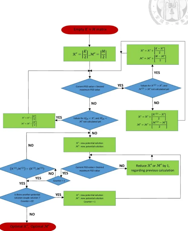
Since the algorithmic sequencing of this section is complex, we propose a flowchart to explain and synthesize the operations performed. The method generally follows the di- agram presented in the previous section, but has been considered for a convergence in two dimensions, which is therefore presented on the following page in the form of a detailed flow chart, indicating the different steps leading to convergence, then the solution of the problem, verifying by a penultimate step, that no potential best couple solution (K′;M′) has not already been calculated.
This last step is an additional calculation performed to ensure that the solution is the best. The fact that we work on a matrix of two dimensions, requires this step of calcula- tion, via the method that we propose, which implies beforehand a research of half-sum, among the couples solutions already calculated, below the desired solution, which could potentially be better, and those above, which are not possible for the user.
Figure 3.1: Sequential flowchart of the proposed method
20
3.3.1 Comparison between Method 3.2 and Method 3.3
Actually the second method, about matrix reshaping from a 2-dimensional matrix to a 1- dimensional one and the third method, which is a 2-dimensional matrix calculation, both methods deserve to be introduced and presented in the thesis, because they all converge to the same results. In addition, the 1-dimensional matrix has precisely a O(KM log KM ) complexity, and the 2-dimensional matrix is about K2M2. A study about the complexity part can be found in [3]. Obviously, the latter method has a higher cost since it requires the last step of calculation, which is to verify that no better potential couple solution has already been calculated.
However, we previously noticed that a problem by choosing the right couple (K′;M′) when the product obtain by calculating the objective function give the same result, was induced. Specifically, we found a conjecture about the settlement of those parameters, which is such that the number of used subcarriersK′ is the largest, and respectively, the number of subsymbolsM′ must be the smallest, so that to reduce the possibility of same result for different couples (K′;M′) in order to guarantee the resolution of the maximum out-of-band PSD.
That is why the last method is present here, because it permits the algorithm to favour the direction of calculation. To be more precise, the conjecture proposes thatM′ is very small in front ofK′so that the second method (1D-matrix) is faster than Method 3.3 (2D- matrix) and would therefore require fewer calculations. Conversely, whenK′is very close toM′, the method does not work and is therefore the limit we find to problem solving through this method. The second method is thus really useful for some narrow cases. Fi- nally, it thus introduces some limits about both last methods, since this calculation problem is already known, but the literature does not propose a clever method yet.
Chapter 4
Results and discussion
Through the resolution method introduced in 5, and by conscientiously following the al- gorithms presented in the previous chapter, we are able to present the problem (2.9) results for different numerical values. Specifically, we need to know the utilization of the CVX tool [7] to understand how our algorithm works under the specific constraints, especially (2.9c). In order to define the out of band partBO of our filters, we define a discretiza- tion on f about 1/(16DTs) Hz. Thus, in order to have a good shape representation of the prototype filters involved, we choose to setBOis defined as :
BO = (
−∞;−K′+ 2 16Ts
)
∪
(K′ + 2 16Ts ;∞
)
We can note therefore that we will not obtain a result for cases whereK′ = K, which can be understood and used as a guard subcarrier, even if the calculation can be run well for upper values of K′ and M′, that is to say the problem can always be solved. The prototype filter is normalized, and the sets of used subcarriers K and used subsymbols M, are changed regarding the method used. For the Method 3.1, using raw force, the numbers of used subcarriersK′ and used subsymbolsM′ are set to the minimum value, and increased one by one in order to complete the empty matrix. Precisely, the value of M′ is firstly increased from 1 to M , before the value ofK′is increased from 0 to K− 1.
The Method 3.2 and 3.3, as mentioned in the Algorithm 3 and the following flowchart, has an initialization ofK′ =⌈K/2⌉ and M′ =⌈M/2⌉.
The other parameters used for the constraint (2.9c) follow the ones introduced in [4].
The results are translated into decibels to have a more physical aspect of the result ob- tained by the constraints of the problem (2.9). Then, in all the results, the desired solution corresponding to ρ in the constraint (2.9c) has been fixed arbitrarily to−27 (dB). To avoid confusion, this is the value that the user does not want to exceed in maximizing the out- of-band PSD of the signal transmitted by the prototype filter. Also, to facilitate reading of results of the problem in 2D matrices involving the results of the PSD out of band, the first row and the first column of each matrix indicate the number of used subcarriersK′ and used subsymbolsM′ involved in the calculation.
4.1 Simulation results
4.1.1 Method 3.1: complete calculation by raw force
Algorithm 1
In this case, K = 10 and M = 5. We can verify in the following table that, whileK′ and M′ are incrementing, the value of the out of band PSD the function is well non- decreasing. We propose in the following table to see the product ofK′ andM′ obtained
24
for the objective function of the problem (2.9) :
1 2 3 4 5 6 7 8 9 10
2 4 6 8 10 12 14 16 18 20
3 6 9 12 15 18 21 24 27 30 4 8 12 16 20 24 28 32 36 40 5 10 15 20 25 30 35 40 45 50
The optimal solution of the problem in this case is therefore 25.
Algorithm 2
Since the Algorithm 2 is based on Algorithm 1, and simply add the changing criterion to redefineK′andM′, the results obtained are obviously the same.
The results introduced in the following subsection, are settled for three cases. In case 1, K = 5 and M = 3, while in case 2, K = 8 and M = 3, and finally in case 3, K = 8 and M = 7. For the Method 3.2, the result should be read in a 1× (K ∗ M) matrix, that is to say read line by line. The two-dimensional reading remains unchanged for Method 3.3.
4.1.2 Method 3.2: 2D to 1D matrix reshaping and Method 3.3: 2D matrix calculation
Case 1 : K = 5 and M = 3
This first case is simple and give a understanding about the results of the given processes of different algorithms. The first matrix is corresponding to second method :
0 0 0 0 0
0 0 −55.97 0 0
0 −37.03 0 −33.67 0
This second matrix is corresponding to the third method :
1 2 3 4 5
1 0 0 0 0 0
2 0 0 −55.97 0 0
3 0 0 −37.03 −33.67 0
Once again, we propose in the following table to see the product ofK′ andM′ obtained for the objective function of the problem (2.9) :
1 2 3 4 5
2 4 6 8 10
3 6 9 12 15
Since the algorithm constantly searches which new couple to calculate according to which it can be a better couple solution (K′;M′) to the problem, that is why no more calculations are needed to find the solution here, to be 12.
26
Case 2 : K = 8 and M = 3
In this case, we propose to improve more the number of used subcarriersK′. The first matrix is corresponding to second method :
0 0 0 0 0 0 0 0
0 0 0 −33.01 0 0 0 0
0 0 −28.54 0 0 −28.03 −26.78 0
This second matrix is corresponding to the third method :
1 2 3 4 5 6 7 8
1 0 0 0 0 0 0 0 0
2 0 0 0 0 −31.26 0 −28.54 0 3 0 0 0 0 0 −28.03 −26.78 0
The following table is about seeing the product ofK′ andM′ obtained for the objective
function :
1 2 3 4 5 6 7 8
2 4 6 8 10 12 14 16 3 6 9 12 15 18 21 24
The result obtained for this case is therefore 18.
Case 3 : K = 8 and M = 7
We now present the last case where the first following matrix is still the second method :
0 0 0 0 0 0 0 0
0 0 0 0 0 0 0 0
0 0 0 0 0 0 0 0
0 0 0 −30.00 0 0 0 0
0 0 0 0 0 0 0 0
0 −27.28 −27.58 −25.54 −26.49 0 0 0
−24.57 0 0 0 0 0 0 0
We notice here the main limitation of the Method 3.2, obtained whenM′ is close toK′. We can not determine precisely in one dimension, when a lot of so many different couple solutions (K′;M′) are present.
As a same schema from the previous cases, we present the Method 3.3 in this case :
1 2 3 4 5 6 7 8
1 0 0 0 0 0 −32.80 0 0
2 0 0 0 0 0 0 0 0
3 0 0 0 0 0 −28.03 0 0
4 0 0 0 0 −28.24 −26.78 −25.54 0
5 0 0 0 0 −27.28 0 0 0
6 0 0 0 −28.24 −26.49 −25.02 0 0
7 0 0 0 −27.58 0 0 0 0
The final table is to determine the product ofK′andM′obtained for the objective function
28
:
1 2 3 4 5 6 7 8
2 4 6 8 10 12 14 16
3 6 9 12 15 18 21 24
4 8 12 16 20 24 28 32 5 10 15 20 25 30 35 40 6 12 18 24 30 36 42 48 7 14 21 28 35 42 49 56
The result obtained for this case is therefore 28.
4.2 Limits of the methods and discussion
Other simulations that are not appropriate for the presentation suggest strongly that the number of used subcarriersK′ has to be really important face to the number of used sub- symbols M′ in order to be efficient, guarantee to maximize the out of band PSD, and furthermore, being more efficient that the last method. since the Method 3.2 is easy to understand and determine how it works. A few narrow cases, such as the Case 1, are how- ever working for this method, since we do not meet so many times different couples for a same result obtained for the objective function.
And that is precisely there that we finally expect to propose the last method (Method 3.3) which promises to be strong and efficient in calculation, and sure to find the results.
Knowing the already calculated values, the algorithm still compare them with the last cal- culated value, in order to see where a new potential solution should be encountered, in order to satisfy the resolution of the problem (2.9). We expect finally helping and propos- ing the literature another line of study in order to develop and advance in the search for solutions to this known problem.
Unfortunately, the limitation of the computer’s memory capacity does not allow us to offer more calculation results for much larger matrices, especially for Method 3.2. How-
ever, Method 3.3 will use the same process to solve the calculation for larger matrices, whose memory usage is different.
30
Chapter 5 Conclusion
In this thesis, we used a matrix-based characterization of generalized frequency division multiplexing (GFDM), in order to design and improve prototype filters used here to max- imize the spectral efficiency. This characterization used properties derived from the con- ventional GFDM matrix transmitter, which were not easily exploitable from the conven- tional filter prototypes observed in the research. From here, we settled to manage the sets of used subcarriers K and used subsymbols M, in order to maximize the spectral effi- ciency in out of band.
In addition, the new optimization problem introducing, firstly solved by raw force, the product maximization of used subcarriers and used subsymbols for out-of-band radiation was addressed under two other main aspects: one resolution in one dimension, and the other in two dimensions. The results showed in the first case and for objective function values having the same result, that the higher the number of used subcarriersK′ is, the better the maximization result will be. Thus, we will choose to maximize this number of used subcarriersK′, within the physical limit possible, to keep an convenient compromise between the devices to maintain and maximize out-of-band spectral efficiency.
The third method, for its part, proposes a solution as convergent as the second, but currently requiring a much larger number of calculations than for the first method, in or- der to solve the proposed maximization problem (2.9).
Moreover, we have emphasized that a good management and design of pairing the couples given by used subcarriers and used subsymbols does permit the maximization of spectral efficiency, a demonstration of this is given is more detailed in the following 5. The contribution involved by this work thus show that an improvement can be studied and developed in order to brighten and perfect the utilization of various prototypes already encountered in the literature, whose primary choice of parameters studied in our main ob- jective function was not adequately defined.
For possible further work, a search for a new effective method for rapid calculation this type of problem certainly already encountered but not yet solved in a formal way, leading to a convergence known in advance. Also, other mathematical methods can be introduced in order to decrease, even drastically and effectively reduce the logarithmic complexity involved in this maximization calculation for a non-decreasing function in both directions (two-dimensional matrix). In view of the memory problem encountered for very large matrices, it could also be envisaged to propose other means of calculation in order to accommodate a larger number of users on a large scale.
32
Bibliography
[1] G. Fettweis, M. Krondorf, and S. Bittner. GFDM - generalized frequency division multiplexing. Veh. Technol. Conf., 2009. VTC Spring 2009. IEEE 69th, pages 1–4, 04 2009.
[2] N. Michailow, M. Matthé, I. Gaspar, A. Caldevilla, L. Mendes, A. Festag, and G. Fet- tweis. Generalized frequency division multiplexing for 5th generation cellular net- works. IEEE Trans. Commun., 62(9):3045–3061, 09 2014.
[3] Po-Chih Chen, Borching Su, and Yenming Huang. Matrix characterization for GFDM:
Low complexity MMSE receivers and optimal filters. IEEE Transactions on Signal Processing, 65(18):4940–4955, 06 2017.
[4] Po-Chih Chen and Borching Su. Filter optimization of out-of-band radiation with performance constraints for GFDM systems. Signal Processing Advances in Wireless Communications (SPAWC), 12 2017.
[5] Ghaith Al-Juboori, Evgeny Tsimbalo, Angela Doufexi, and Andrew R. Nix. A com- parison of OFDM and GFDM-based MFSK modulation schemes for robust IoT ap- plications. 2017 IEEE 85th Vehicular Technology Conference (VTC Spring), 11 2017.
[6] M. Matthé, N. Michailow, I. Gaspar, and G. Fettweis. Influence of pulse shaping on bit error rate performance and out of band radiation of generalized frequency division multiplexing. Proc. IEEE ICC Workshop, pages 43–48, 2014.
[7] M. Grant and S. Boyd. Cvx: Matlab software for disciplined convex programming, version 2.1.
[8] S. Boyd and L.Vandenberghe. Convex Optimization. Cambridge University Press, 2009.
[9] J. Dattorro. Convex optimization Euclidean distance geometry. Meboo Publishing, 2016.
34
Power Spectral Density and OOB Leakage
In this section, which serves as an aid for simulation later, we define the OOB leakage O as a performance measure for the OOB radiation of transmit signals. To evaluate O for GFDM, we first address the power spectral density (PSD) of GFDM signals. We derive an analytical PSD expression encompassing an interpolation filter used in a D/A converter.
Actually, from the GFDM digital baseband transmit signal x[n], we obtain the analog baseband transmit signal xa(t) is obtained by passing x[n] through a D/A converter with a sampling interval Ts and an interpolation filter p(t), id est, xa(t) = ∑∞
n=−∞x[n]p(t− nTs). The PSD of xa(t) is defined as Sa(f ) = limT→∞E{2T1 |∫T
−T xa(t)e−j2πftdt|2}. Let P (f ) =∫∞
−∞p(t)e−j2πftdt be the Fourier transform of p(t), and Gm(ejw) =∑∞
n=−∞
gm[n]e−jwn be the discrete-time Fourier transform of gm[n], where gm[n] is defined in (2.7). Assuming the data symbols are zero-mean and i.i.d. with symbol energy ES, we can derive that
Sa(f ) = ES|P (f)|2 D′Ts
∑
k∈K
∑
m∈M
Gm
(
ej2π(f Ts−Kk)) 2. (1) With some derivations, we further obtain that
Gm(ejw) =
D∑′−1 l=0
[ g(m)f
]
l
sincD′(wl′)e−jwl′D′2−1, (2)
where wl′ = w− (2πl/D′) and [
g(m)f ]
l = D D′
D∑−1 k=0
{
[gf]ksincD′
( 2π
(k D − l
D′ ))
ejπ(Dk−D′l )(D′−1)e−j2πkmK+LD }
. (3)
Since gf is the frequency-domain prototype transmit filter, defined as the D-point DFT of g, id est,
gf =√
DWDg, (4)
and
sincp(x) =
(−1)k(p−1), x = 2πk, k∈ Z sin(px/2)
p sin(x/2), otherwise
(5)
is the periodic sinc function for any positive integer p. Using (1), (2), (3) and (4), we can express the PSD with gf, which enables designing the PSD in terms of the frequency- domain prototype transmit filter. A special case that leads to a simple expression of Gm(ejw) is L = 0. When L = 0, (2) can be reduced to
Gm(ejw) =
D∑−1 l=0
[gf]le−j2πlmMsincD(wl)e−jwlD−12 , (6)
where wl = w− (2πl/D).
To characterize the OOB radiation, we define the OOB leakage as
O = |BI|
|BO| ·
∫
f∈BOSa(f ) df
∫
f∈BISa(f ) df . (7)
In (7),BOandBIare the set of frequencies considered out of band and in band respec- tively, and|BO| and |BI| denote the lengths of the corresponding intervals. Recall that K is the set of subcarrier indices actually used. The nominal frequencies of the subcarriers inK lie in BI, several guard subcarriers are used betweenBOandBI, andBOis reserved
36
for the use of other users.
Finally, note that in (2.6), the setsK and M are not required to be K = {0, 1, · · · , K − 1} or M = {0, 1, · · · , M − 1}. This means some guard symbols or guard subcarriers can be used. GFDM is proposed to exhibit low OOB radiation. This advantage is particularly significant if some guard symbols and guard subcarriers are used [6].