A Comparative Study of Two High Performance Current Control Techniques for Three-Phase Shunt Active Power Filters

A Comparative Study of Two High Performance Current Control Techniques for Three-Phase Shunt Active Power Filters

Wanchak Lenwari

Dept. of Control System and Instrumentation Engineering

King Mongkut’s University of Technology Thonburi Bangkok, Thailand

wanchak.len@kmutt.ac.th

Milijana Odavic

Dept. of Electrical and Electronic Engineering The University of Nottingham

Nottingham, United Kingdom milijana.odavic@nottingham.ac.uk

Abstract -- In recent years, the increase of non-linear loads in electrical power system has sparked the research in power quality issue. The shunt active power filter (SAPF) is a power electronic device which has been developed to improve power quality. The current control of shunt power filters is critical since poor control can reinforce existing harmonic problems.

Various control strategies have been proposed by many researchers. In this paper, a comparative evaluation of the performance of two current control techniques, resonant and predictive controller, is presented with identical system specification. The design procedure and principle of both current control methods are also presented in detail. Simulation results show the comparison of transient response, steady state control and performance in the presence of variation of supply impedance between two control techniques.

Index Terms--active filters; power quality; power system harmonics; current control; resonant controller; predictive controller

I. I NTRODUCTION

There are two types of loads in electrical power systems, linear and non-linear loads. A linear element in a power system is a component in which the current is proportional to the voltage. On the other hand, the current shape of a non- linear load is not the same as the voltage. Nowadays, non- linear loads are a major source of harmonic generation for most power networks and can cause resonance problems and degrade the power quality, in particular, rectifiers which are commonly used in switched mode power supplies for many domestic appliances. In addition, rectifiers are extensively used as interface circuits for power electronics system in industry. The conventional method to filter out the harmonics is to use tuned passive filters but active power filters have superior in filtering performance.

An active power filter has two main configurations: 1) Shunt configuration which the filter is connected in parallel with harmonic loads and 2) Series configuration which the filter is connected in series with the loads. Considering harmonic cancellation basic idea, shunt active filter injects current to directly cancel polluting current while series active filter compensate the voltage distortion caused by non-linear

loads. This paper will focus on the control of shunt active power filters which has been widely used to improve power quality. The performance of active filter is dependent on two parts: the harmonic reference generation and current control system.

A vast variety of current control methods for active power filters has been introduced by many researchers in order to track the reference currents with the lowest possible error which is the main target for all harmonic compensations [1]- [3]. These methods are hysteresis control [4], predictive control [5]-[11], resonant control [12]-[15], instantaneous reactive power theory [16], and repetitive control [17]-[18].

Among current control techniques, resonant based compensator and predictive based compensator appear to be suitable for active filter control as both provide precise control and good speed of response. This leads to the main objective of this paper which aims to evaluate and compare both current control schemes. This paper presents the comparative performance evaluation of these two high performance current control strategies: resonant based compensator and predictive based compensator. Comparison criteria considered here is based on the control performance.

The design procedures and principles of two control techniques are discussed here. The simulation results of the comparison are presented, which is done according to the identical system parameter.

II. C ONTROL OF S HUNT A CTIVE P OWER F ILTER

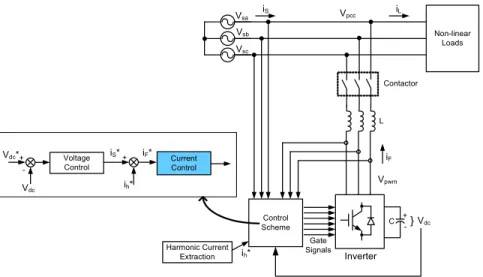
The standard shunt active filter has the structure illustrated

in Fig. 1 where control structure consists of two control loops,

dc voltage control (outer loop) and current control (inner

loop) which mainly determines the filtering performance. The

output voltage of the inverter, V pwm , is controlled with respect

to the voltage at the point of common coupling, V pcc , to force

the output current (i F ) to match harmonic reference values

obtained from harmonic current extraction methods. The

voltage loop has a bandwidth which is much smaller than that

of current control hence it can cause no interference to current

controller performance investigated in this paper. Resonant

based compensator and predictive based compensator are

discussed as follows.

C + -

Non-linear Loads

Current Control

Gate Signals Voltage

Control

V

_pcc

V

sa

V

_sb

V

_sc

V

pwm

L

Harmonic Current Extraction i

h

* +

}

+ -

V

dc

V

dc

*

Inverter Contactor

i

L

i

S

Control Scheme V

dc

i

S

* i

F

* i

F

i

_h

*

Fig. 1. The structure of three-phase shunt active filter

0 5 10 15 20 25 30 35

M agnit ud e (dB)

10

¹

10

²

10

³

10

⁴

10

⁵

Frequency (rad/sec)

+ + + _

i

dq_ref

(n)

z ⁻ 1 ^I

^dq

^(t)

Computation Delay

+ ZOH

PWM Inverter

1 Ls R +

T

s

i

dq

(n)

d cz z

b az

+

−

−

2

f ez z

d cz

+

−

−

2

K

P

Active Filter

A. Design of Resonant Based Current Control

The resonant compensator was developed to accurately control the signal at resonant frequency, whilst rejecting all other frequencies. The basic controller is given in (1) [12]- [13].

∑ ₊

+

=

h

ih

p s h

s K K

s

C _{2 2}

) . ( ) .

( ω ⁽¹⁾

The compensator provides a very high gain at the tuned resonance frequencies thus zero or quasi-zero steady state error can be achieved. Another advantage of this control scheme is the ability to eliminate the signal having the same frequency as the tuned resonance frequencies which act as external disturbance to the current control system. In order to precisely design a controller, the modified transfer function of resonant controller is proposed in [14]-[15] as expressed in (2) where K p and K rh are the gain of proportional term and each resonant term respectively while Q is a quality factor of resonant term.

∑ _{+ +}

+

=

h h h h

h rh

p s Q s

s K K

s

C _{2 2}

) ( ) / ( ) .

( ω ω

ω (2)

It is obviously seen that the control parameters in (2) require a complicated design procedure particularly when many harmonics are compensated by a controller. The use of dq frame of reference alleviates this complication since two pairs of harmonics are seen as the same frequency (i.e. 5 ^th and 7 ^th harmonics both appear at 300 Hz) however with a different sign of q-axis component. Therefore, four main harmonics (5 ^th , 7 ^th , 11 ^th , and 13 ^th ) can be controlled by one controller having two resonant frequencies at 300 Hz and 600 Hz as presented by the bode plot in Fig. 2.

Fig. 2. Bode plot of resonant controller having two resonant frequencies at 300 Hz and 600 Hz

Fig. 3. z-domain current control loop in dq frame of reference

In this paper, the design was undertaken in the discrete domain by the discrete root locus of the closed-loop system considering one computation delay as shown in Fig. 3. The PWM inverter was represented by a zero-order hold.

In addition, the continuous time is discretized by using a

forward rectangular approximation to obtain all discrete

model including the plant. The choosing of controller

parameters in Fig. 3 requires a complicated procedure and in

this paper, the criteria are based on a similar principle as

presented in [15]. As all designed controller parameters

determine the control performance therefore a compromise

between control accuracy, speed of response, stability and

robustness must be taken into account in the design in particular where the power system impedance is varied.

B. Design of Predictive Based Control

The predictive current controller [10] is designed to be able to work even though the microprocessor incurs a processing time delay. The employed current control approach is based on the following discrete linear model of the system [5]:

L T R b e L T e R

a

b k V k E a k i k i

s sL T R s

sL T

R

≈ − ⋅ = − ≈

=

⋅

− +

⋅

= +

⋅

⋅

− /

, 1 1

)) ( ) ( ( ) ( ) 1

( (3)

where a and b are the coefficients approximated by a Taylor series. The time constant of the ac side of the SAPF is denoted by L/R. The SAPF current at time instants k and k+1 are denoted by i(k) and i(k +1) respectively. In order to design two-steps ahead predictive current controller the discrete SAPF model for the sample period between the time instances k+1 and k+2 can be rewritten from (3) in the following form:

b k V k E a k i k

i ( + 2 ) = ( + 1 ) ⋅ + ( ( + 1 ) − ( + 1 )) ⋅ (4) The SAPF reference voltage (6) can be calculated from (4) by introducing (5). The aim of the controller proposed in this work is to predict the SAPF voltage reference for the next sampling period (between the sampling instants k+1 and k+2) to minimise the current error at the instant k+2, as shown in Fig. 4.

0 ) 2 (

) 2 ( ) 2 ( ) 2

(

^*

≈ + Δ

+ Δ

− +

= + k i

k i k i k

i (5)

[ ^{i k i k a} ]

k b E k

V ( + 1 ) =

_p

( + 1 ) − 1

_p^*

( + 2 ) −

_p

( + 1 ) ⋅ (6) Equation (6) should be calculated during the period between samples k and k+1 and it should be noted that current and voltage values for the next sampling period (i.e.

i(k+1) and E(k+1)) are not available and need to be predicted.

The predicted values of i(k+1), i*(k+2) and E(k+1) are respectively denoted by i p (k+1), i p *(k+2) and E p (k+1). The current reference is predicted two-steps ahead of its appearance using values from a few previous sampling instants. In numerical mathematics, this process of constructing new values outside the known set of discrete data is called extrapolation. Generally a two-ahead extrapolation of the current reference using values from n previous sampling instants can be expressed in the following nth-order discrete form:

) ( ...

) 2 ( ) 1 ( ) ( ) 2

(

2 ^{* *}

* 1

* 0

*

k a i k a i k a i k a i k n

i

p

+ = ⋅ + ⋅ − + ⋅ − + +

n

⋅ − (7)

where a i (i = 0 to n) are the coefficients of the n-order extrapolation. In this work to determine the extrapolation coefficients, the interpolation polynomial in the Lagrange form [10] is used with the advantage that the sampling frequency is constant. However, when a step change occurs a large error is introduced to the prediction for the next few sampling instants depending on the order of the extrapolation used. To decrease this effect, when a reference change is detected the prediction over the next few sampling instants can be frozen; the current reference value at the instant of change can be used instead.

t k T s t k+1

i _k i* _k

V k+1

i k+1

t k+2

T s

i * k+1

i * _k+2 V k

i k+2

t V

i

i _k

Fig. 4. Predictive controller principal

The SAPF current prediction can be defined as [10]:

( )

) 1 ( ) 1 ( ) 1 (

1 ))

( ) 1 ( ( ) ( ) 1 (

*

* *

+

− +

= + Δ

+ Δ +

− + +

= +

k i k i k i

k i k i k i k i k i

p p

p

p

(8)

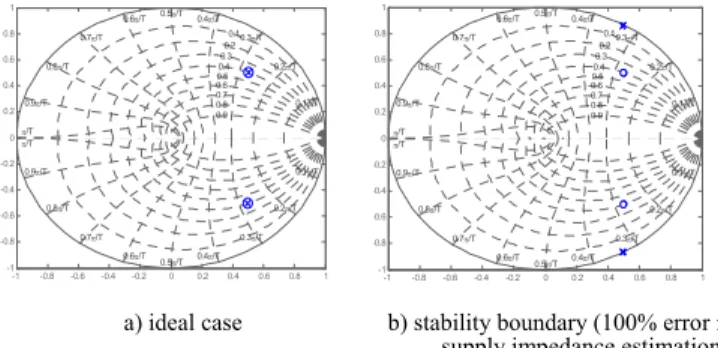
The performance of the analyzed predictive current controller, which is a model-based controller, depends on the accuracy of the model parameters used. The pole-zero placement of the closed current control loop is shown in Fig.

5. If the modeled input impedance of the system perfectly matches the actual value, the SAPF current will follow the reference value without introducing any delay, Fig. 5a. The system remains stable for all underestimates of the input inductance [10]. Overestimates in the input inductance are tolerated until a 100% error is reached, Fig. 5b. This stability analysis therefore shows the control has very good robustness to parameter inaccuracy.

-1 -0.8 -0.6 -0.4 -0.2 0 0.2 0.4 0.6 0.8 1

-1 -0.8 -0.6 -0.4 -0.2 0 0.2 0.4 0.6 0.8 1

0.1π/T 0.2π/T 0.3π/T 0.4π/T 0.5π/T 0.6π/T 0.7π/T 0.8π/T

0.9π/T π/T

0.1π/T

0.2π/T

0.3π/T 0.4π/T 0.5π/T 0.6π/T 0.7π/T 0.8π/T 0.9π/T π/T

0.1 0.2 0.3 0.4 0.5 0.60.7 0.8 0.9

^{-1-1 -0.8 -0.6 -0.4 -0.2 0 0.2 0.4 0.6 0.8 1}

-0.8 -0.6 -0.4 -0.2 0 0.2 0.4 0.6 0.8 1

0.1π/T 0.2π/T 0.3π/T 0.4π/T 0.5π/T 0.6π/T 0.7π/T 0.8π/T

0.9π/T π/T

0.1π/T

0.2π/T

0.3π/T 0.4π/T 0.5π/T 0.6π/T 0.7π/T 0.8π/T 0.9π/T π/T

0.1 0.2 0.3 0.4 0.5 0.6 0.7 0.8 0.9

a) ideal case b) stability boundary (100% error in supply impedance estimation )

Fig. 5. Poles-zeros placement for the proposed predictive controller as

L varies

III. C OMPARISON R ESULTS

The SAPF model including the control systems were simulated using Matlab-Simulink and the Simpowersystem toolbox. Shunt active power filters and common parameters used for simulation are shown in Table I. The comparison results between two control techniques presented are as follows: Fig. 6 shows steady state control of both 5 ^th (5A) , 7 ^th (3A) , 11 ^th (1A) and 13 ^th (0.5A) harmonics combined. Fig. 7 shows the steady state control of 5 ^th (5A) , 7 ^th (3A) , 11 ^th (1A) and 13 ^th (0.5A) harmonics together in the presence of variation of supply impedance. The transient response to a step change is investigated as shown in Fig. 8 where the 5 ^th harmonic current reference is changed from 0A to 5A at time 0.5 second.

IV. C ONCLUSION

This paper has presented the comparative study in the control performance of the two high performance current control systems for shunt active filtering. The comparison is carried out by simulating. For steady state control, results show excellent accurate harmonic control for both current control systems with very small magnitude and phase errors.

For transient response, predictive control provides a considerable error according to its algorithm used the previous data to predict signals. Techniques can be applied to improve this poor transient behavior. For design consideration, the performance of resonant based control is determined by controller parameters and to obtain these parameters is relatively complicated particularly when higher order harmonic compensation is required. Instead, the predictive based control is less complicated regarding the design procedure and can control many harmonics, not only the selected harmonics. On-going work is looking at a practical comparison and performance evaluation of more current controllers.

R EFERENCES

[1] H. Akagi, “New trends in active filters for power conditioning,” IEEE Trans. Industry Application, vol. 32, pp. 1312–1322, November/December 1996.

[2] S. Buso, L. Malesani, and P. Mattavelli, “Comparison of current control techniques for active filter applications,” IEEE Trans.

Industrial Electronics, vol. 45, no. 5, pp. 722 – 729, October 1998.

[3] B. Singh, K. Al-Haddad, and A. Chandra, “A review of active filters for power quality improvement,” IEEE Trans. Industrial Electronics, vol. 46, no. 5, pp.960 – 971, October 1999.

[4] L. Malesani, P. Mattavelli, and P. Tomasin, “High-performance hysteresis modulation technique for active filters,” IEEE Trans. Power Electronic, vol. 12, no. 5, pp.876–884, September 1997.

[5] Osman Kukrer, “Discrete-Time current control of voltage-fed three- phase PWM inverters,” IEEE Trans. Power Electronics, vol. 11, pp.

260–269, March 1996.

[6] D. G. Holmes and D. A. Martin, “Implementation of a Direct Digital Predictive Current Controller for Single and Three Phase Voltage Source Inverters,” in Conf. Rec. IEEE-IAS Annu. Meeting, San Diego, October 1996, pp. 906-913.

[7] Seung-Gi Jeong, Myung-Ho Woo, “DSP-Based Active Power Filter with Predictive Current Control,” IEEE Trans. on Industrial Electronics, vol. 44, no. 3, pp. 329–336, June 1997.

[8] Mohammad Sedighy, Shashi B. Dewan, Francis P. Dawson, “A robust digital current control method for active power filters,” IEEE Trans.

Industrial Applications, vol. 36, no.4, pp.1158-1164, July/August 2000.

[9] H. Abu-Rub, J. Guzinski, Z. Krzeminski and H.A.Toliyat, “Predictive current control of voltage source inverters,” IEEE Trans. Industrial Electronics, vol. 51, no.3, pp.585–593, June 2004.

[10] M. Odavic, P. Zanchetta, M. Sumner, “A “Two ahead” Predictive Controller for Active Shunt Power Filters,” in Proc. of 32nd Annual Conference of the IEEE Industrial Electronics Society, IECON’06, Paris, France, pp. 4713–4718.

[11] J. Rodriguez, J. Pontt, C. A. Silva, P. Correa, P. Lezana, P. Cortes, U.

Ammann, “Predictive current control of a voltage source inverter”, IEEE Trans. Industrial Electronics, vol.54, no. 1, pp. 495-503, February 2007.

[12] D.N. Zmood, D.G. Holmes, and G. Bode, “Frequency domain analysis of three phase linear current regulators,” IEEE Trans. Industry Application, vol. 37, no. 2, pp. 601– 610, March/April 2001.

[13] M. Liserre, R. Teodorescu, and F. Blaabjerg, “Multiple harmonics for three-phase grid converter systems with the use of PI+RES current controller in a rotating frame,” IEEE Trans. Power Electronics, vol.

21, No. 3, pp. 836 – 841, May 2006.

[14] W. Lenwari, M. Sumner, P. Zanchetta, and M. Culea, “A high performance harmonic current control for shunt active filters based on resonant compensators” in Proc. of 32nd Annual Conference of the IEEE Industrial Electronics Society, IECON’06, Paris, France, pp.

2109–2114.

[15] W. Lenwari, M. Sumner, and P. Zanchetta, “The use of genetic algorithms for the design of resonant compensators for active filters,”

IEEE Trans. Industrial Electronics, vol. 56, no. 8, pp. 2852 – 2861, August 2009.

[16] R.S. Herrera, P. Salmeron, and Hyosung Kim, “Instantaneous Reactive Power Theory Applied to Active Power Filter Compensation: Different Approaches, Assessment, and Experimental Results,” IEEE Trans.

Industrial Electronics, vol. 55, no. 1, pp. 184–196, January 2008.

[17] R. Grino, R. Cardoner, R. Costa-Castello, and E. Fossas, “Digital Repetitive Control of a Three–Phase Four-Wire Shunt Active Filter,”

IEEE Trans. Industrial Electronics, vol. 54, no. 3, pp. 1495-1503, March 2007.

[18] B. Cheowait, B. Panomruttanarug, and W. Lenwari, “Design and Analysis of Current Control for Shunt Active Filter Based on Repetitive Control Technique using Optimization in the Frequency Domain” in Proc. of the IEEE International Conference on Robotic and Biomimetic(ROBIO 2008), Bangkok, Thailand, pp. 871– 876.

TABLE I

S HUNT A CTIVE P OWER F ILTER AND C OMMON P ARAMETERS Shunt Active Power Filter: 5mH, 0.4Ω

AC Input Voltage: 120Vrms, 50Hz

DC-link PI Controller: (0.3z-0.295)/(z-1)

Vdc*: 400V

DC-link Capacitor: 1000 µF

Sampling Frequency: 5kHz

Switching Frequency: 5kHz

0.5 0.52 -10

-5 0 5 10

Time(s)

C u rre n t(A )

i _real i _ref

Resonant Control

0.5 0.52

-10 -5 0 5 10

Time(s)

Cu rr e nt (A)

Resonant Control

i _real i _ref

0.5 0.52

-10 -5 0 5 10

Time (s)

Cu rr en t (A )

Predictive Control

i ref i real

^{0.5 0.52}

-10 -5 0 5 10

Time (s)

C ur rent ( A )

i real

i ref Predictive Control

Fig. 6. 5th,7th, 11th, and 13th harmonic control. Fig. 7. 5th,7th, 11th, and 13th harmonic control in the presence of supply inductance variation(+20%)

0.5 0.52 0.54 0.56

-5 0 5 10

Time(s)

Cu rr e n t( A )

Resonant Control i _ref

i _real

0.5 0.51 0.52 0.53 0.54 0.55 0.56

-5 0 5 10

Time (s)

C urre nt (A)

Predictive Control i real

iref

Fig. 8. Step response to a change in 5th harmonic reference