嵌入式奈米石墨烯板三維非局部彈性力學漸近理論之發展與應用

全文

(1)科技部補助專題研究計畫成果報告期末報告. 嵌入式奈米石墨烯板三維非局部彈性力學漸近理論之發展與應用(第3年). 計計執執. 畫畫行行. 類編期單. 別號間位. ：：：：. 個別型計畫 MOST 106-2221-E-006-036-MY3 108年08月01日至109年07月31日國立成功大學土木工程學系（所）. 計畫主持人：吳致平計畫參與人員：博士班研究生-兼任助理：李維宸. 本研究具有政策應用參考價值：■否 □是，建議提供機關（勾選「是」者，請列舉建議可提供施政參考之業務主管機關）本研究具影響公共利益之重大發現：□否 □是中華民國 109 年 06 月 17 日.

(2) 中文摘要：本計畫擬以三年為期，分別應用微擾方法和多尺度方法，發展非局部彈性力學漸近解析方法，並將其應用於嵌入式單層與多層式奈米石墨烯板結構之三維振動和挫屈等力學問題，發展之方法將以傳統文獻既有之SLGS和MLGS結構靜動態問題之精確解進行驗證，爾後再針對傳統文獻欠缺之SLGS和MLGS結構各類結構行為進行參數分析與預測。計畫中第一年之研究工作聚焦於:(1) 結合微擾方法和多時間尺度方法，在基於三維非局部彈性力學理論架構下，發展適用於SLGS奈米結構自然振動分析之三維漸近理論與解析方法。在理論推衍中，該嵌入式奈米尺度石墨烯板結構與其周遭之高分子材料間之互制效應將以具二參數之Pasternak基礎模式模擬之。該自然振動問題之時間場量變數假設為簡諧函數，x-y平面域內之空間變數則以雙傅立葉函數模擬之，文獻中極為少數之標準驗證範例精確解，則用以評估該三維解析方法之精確與收斂率。計畫中第二年之研究工作聚焦於(2) 結合微擾方法和多尺度方法，在基於三維非局部彈性力學理論架構下。發展適用於SLGS奈米結構受雙軸壓力作用下，挫屈分析之三維漸近理論與解析方法。同樣的，在理論推衍中，該嵌入式奈米尺度石墨烯板結構與其周遭之高分子材料間之互制效應將以具二參數之Pasternak基礎模式模擬之。該挫屈問題之x-y平面域內之空間變數將以雙傅立葉函數模擬之，臨界挫屈參數則展開成多尺度挫屈參數之級數解形式。在高階問題中將引入可解條件和歸一化條件，以消除奇異項，並進而求得唯一解。文獻中極為少數之標準驗證範例精確解，則用以評估該三維解析方法之精確與收斂率。計畫中第三年之研究工作聚焦於(3) 引入奈米石墨烯板層與層間之凡得瓦爾力，延伸第一和第二年單層奈米石墨烯板結構之三維靜動態漸近理論與解析方法之研究成果。進而發展適用於多層奈米石墨烯板結構靜動態問題之漸近理論與解析方法，理論分析中將針對目前既有文獻中之二類凡得瓦爾力互制模式進行比較，探討其影響。中文關鍵詞：挫屈，振動，石墨烯板，多尺度方法，微擾方法，凡得瓦爾力。英文摘要： This proposal is organized as a three-year-term project. Based on the perturbation method and the method of multiple scales, we developed the three-dimensional (3D) asymptotic nonlocal elasticity theory for various 3D vibration and stability analyses of single-layered (SL) and multi-layered (ML) graphene sheets (GS) embedded in an elastic medium. The asymptotic solutions will be compared with the accurate solutions of some benchmark problems available in the literature to assess the accuracy and convergence rate of the current asymptotic theory. In the first year, the research work focused on “Development of the 3D asymptotic nonlocal elasticity theory and its application to the 3D free vibration analysis of simply supported, SLGS embedded in an elastic medium”. In the formulation, the interaction between the SLGS and its surrounding medium was modelled as a two-.

(3) parameter Pasternak foundation. The time variable was expanded as a power series of a perturbation parameter with different time scales. The variations of assorted field variables in time domain were assumed to be a harmonic function, while those in the in-plane domain were expanded the double Fourier series functions. Some benchmark solutions available in the literature were used to estimate the accuracy and convergence rate of the current asymptotic theory. In the second year, the research work focused on “Development of the 3D asymptotic nonlocal elasticity theory and its application to the 3D buckling analysis of simply supported, SLGS embedded in an elastic medium and under bi-axial compressive loads”. In the formulation, the interaction between the SLGS and its surrounding medium was modelled as a two-parameter Pasternak foundation. The critical load was expanded as a power series of a perturbation parameter. The variations of assorted field variables in the in-plane domain were expanded the double Fourier series functions. The solvability and normality conditions were introduced in order to eliminate the secular terms in the higher-order problems and to obtain a unique solution. Some benchmark solutions available in the literature were used to estimate the accuracy and convergence rate of the current asymptotic theory. In the last year, the research work focused on “Development of the 3D asymptotic nonlocal elasticity theory and its application to the 3D free vibration and buckling analyses of simply supported, MLGS embedded in an elastic medium”. In the formulation, the results of first two years for the analysis of SLGS were extended to the analyses of MLGS by introducing the van der Waals (vdW) interactive force between adjacent layers constituting the MLGS. Two vdW interaction models given by He et al. and Ru were introduced, and the results obtained using these two vdW interaction models were compared with each other. 英文關鍵詞： Buckling, vibration, graphene sheets, multiple scale methods, perturbation methods, van der Waals interaction..

(4) 行政院科技部科學委員會補助專題研究計畫成果報告. 嵌入式奈米石墨烯板三維非局部彈性力學漸近理論之發展與應用 Development and Application of the 3D Nonlocal Asymptotic Elasticity Theory of Embedded Nanoscale Graphene Sheets. 計畫編號：MOST 106-2221-E-006-036-MY3 執行時間：106 年 8 月 1 日至 109 年 7 月 31 日主持人：吳致平教授執行機構及系所：國立成功大學土木工程學系.

(5) Abstract This project was organized as a three-year-term one. On the basis of the Eringen nonlocal elasticity theory and multiple time scale method, we aimed to developing an asymptotic approach for three-dimensional (3D) bending, buckling and the cylindrical bending vibration analysis of simply-supported nanoplates and graphene sheets (GSs) embedded in an elastic medium. Nonlocal classical plate theory (CPT) is derived as a first-order approximation of the 3D nonlocal elasticity theory, and the motion equations for higher-order problems retain the same differential operators as those of nonlocal CPT, although with different nonhomogeneous terms. In the first year, the research work focused on “Free vibration analysis of embedded single-layered nanoplates and graphene sheets by using the multiple time scale method”. In the formulation, the small length scale effect is first introduced to the nonlocal constitutive equations by using a nonlocal parameter, then the mathematical processes of nondimensionalization, asymptotic expansion and successive integration are performed, and finally recurrent sets of motion equations for various order problems are obtained. The interactions between the nanoplates (or GSs) and their surrounding medium are modelled as a two-parameter Pasternak foundation. Some 3D nonlocal elasticity solutions of the natural frequency parameters of nanoplates (or GSs) with and without being embedded in the elastic medium and their corresponding through-thickness distributions of modal field variables are given to demonstrate the performance of the 3D asymptotic nonlocal elasticity theory. In the second year, the research work focused on “Asymptotic nonlocal elasticity theory for the buckling analysis of embedded single-layered nanoplates/graphene sheets under biaxial compression”. In the formulation, the Eringen nonlocal elasticity theory is used to capture the small length scale effect, and the interaction between the SLNP/SLGS and its surrounding medium is simulated using a Pasternak-type foundation. After performing the mathematical processes of nondimensionalization, asymptotic expansion and successive integration, we finally obtain recursive sets of governing equations for various order problems. Some accurate nonlocal elasticity solutions of the critical load parameters of simply-supported, biaxially-loaded SLNP/SLGS with and without being embedded in the elastic medium are given to demonstrate the performance of the 3D asymptotic nonlocal elasticity theory. In the last year, the research work focused on “Cylindrical bending vibration of multiple graphene sheet systems embedded in an elastic medium”. Both the interactions between the topmost and bottommost GSs and their surrounding medium and the interactions between each pair of adjacent GSs are modelled as one-parameter Winkler models with different stiffness coefficients, namely, respectively. In the formulation, the small length scale effect is introduced to nonlocal constitutive equations using a nonlocal parameter, and then the nondimensionalization, asymptotic expansion, and successive integration mathematical processes are performed for a typical GS. After assembling the motion equations for each individual GS to form those of the multiple GS system, finally, recurrent sets of motion equations can be obtained for various order problems. Some nonlocal plane strain solutions for the natural frequency parameters of the multiple GS system with and without being embedded in the elastic medium and their corresponding mode shapes are presented to demonstrate the performance of the asymptotic nonlocal elasticity theory. Keywords: Eringen nonlocal elasticity theory, asymptotic approach, nanoplates, graphene sheets(GSs), asymptotic nonlocal elasticity theory.. I.

(6) Contents Abstract……………………………………………………………………………………………….I Chapter 1 Introduction…………..……………………………………………………………………1 Chapter 2 Free vibration analysis of embedded single-layered nanoplates and graphene sheets by using the multiple time scale method………………………….……….……………….3 2.1 Basic equations of 3D nonlocal elasticity theory……….………….…………………....3 2.2 Nondimensionalization………………………………………………………………….4 2.3 Asymptotic expansion…………………………………………………………………...6 2.4 Asymptotic integration and various order problems……………………………….……7 2.4.1 The 0 -order problem………………………………………………………………...7 2.4.2 The 2 -order problem………………………………………………………………...8 2.5 Applications……………………………………………………………………...…….10 2.5.1 0 -order solution………………………………………………………………..……10 2.5.2 First-order modifications……………………………………………………………..11 2.6 Illustrative examples………………………………………….………………………..12 2.6.1 Isotropic nanoplates………………………………………………………………….12 2.6.2 Isotropic graphene sheets with and without being embedded in the elastic medium..13 Chapter 3 Asymptotic nonlocal elasticity theory for the buckling analysis of embedded single-layered nanoplates/graphene sheets under biaxial compression………………..21 3.1 Basic equations of 3D nonlocal elasticity theory………………………………………21 3.2 Nondimensionalization………………………………………………………………...23 3.3 Asymptotic expansion……………………………………………………….…………24 3.4 Asymptotic integration and various order problems…………………………………...25 3.4.1 The 0 -order problem……………………………………………………………….25 3.4.2 The 2 -order problem……………………………………………………………….26 3.5 Applications……………………………………………………………………………27 3.5.1 0 -order solution……………………………………………………………………..27 3.5.2 First-order modifications……………………………………………………………..28 3.6 Illustrative examples…………………………………………………………………...30 3.6.1 Bending of orthotropic nanoplates…………………………………………………...30 3.6.2 Buckling of isotropic nanoplates……………………………………………………..30 3.6.3 Buckling of single-layered GSs……………………………………………………...31 3.6.4 Buckling of single-layered GS embedded in an elastic medium…………………….31 Chapter 4 Cylindrical bending vibration of multiple graphene sheet systems embedded in an elastic medium………………………………………………………………………………..….39 4.1 Nonlocal Plane Strain Elasticity Theory……………………………………………….39 4.2 Nondimensionalization………………………………………………………………...40 4.3 Asymptotic Expansion…………………………………………………………………41 4.4 Asymptotic Integration and Various Order Problems………………………………….42 4.4.1 The 0 -order problem……………………………………………………………….42 4.4.2 The 2 k -order (k=1, 2, 3, …) problem………………………………………………..43 4.5 Applications……………………………………………………………………………45 4.5.1 0 -order solution……………………………………………………………………..45 4.5.2 First-order modifications…………………………………………………………….46 4.6 Illustrative examples…………………………………………………………………...47 4.6.1 Laminated composite macroplates…………………………………………………...47 4.6.2 Nanobeams…………………………………………………………………………...48 4.6.3 Multiple GS systems…………………………………………………………………48 II.

(7) Chapter 5 Conclusions………………….………………………………………………………..….58 Chapter 6 References………………………………………………………………......……………60. III.

(8) Table Contents Table 2.1…………………………………………………………………….………………………15 Table 2.2……………………………………………………………………….……………………16 Table 3.1………………………………………………………………………….…………………33 Table 3.2………………………………………………………………………………….…………34 Table 3.3…………………………………………………………………………………………….35 Table 4.1…………………………………………………………………………………………….50 Table 4.2…………………………………………………………………………………………….51 Table 4.3…………………………………………………………………………………………….52. IV.

(9) Figure Contents Figure 2.1……………………………………………………………………………………………17 Figure2.2…………………………………………………………………………………………….18 Figure2.3…………………………………………………………………………………………….19 Figure2.4…………………………………………………………………………………………….19 Figure2.5…………………………………………………………………………………………….20 Figure2.6…………………………………………………………………………………………….20 Figure 3.1……………………………………………………………………………………………36 Figure 3.2……………………………………………………………………………………………37 Figure 3.3……………………………………………………………………………………………38 Figure 3.4……………………………………………………………………………………………38 Figure 4.1……………………………………………………………………………………………53 Figure 4.2……………………………………………………………………………………………54 Figure 4.3……………………………………………………………………………………………54 Figure 4.4……………………………………………………………………………………………55 Figure 4.5……………………………………………………………………………………………56 Figure 4.6……………………………………………………………………………………………57. V.

(10) Chapter 1 Introduction In recent years, the fields of nanoscience and nanotechnology have developed significantly, since some nanostructured elements, such as the beam-like (or circular hollow cylinder-like) carbon nanotubes (CNTs) [1] and plate-like graphene sheets (GSs) [2], were first discovered. Due to their excellent mechanical, chemical, thermal and electrical material properties, CNTs and GSs have thus been introduced in a variety of potential applications to both micro- and nano-electro-mechanical systems (MEMs and NEMs), such as communication, machinery, information, and biological technologies [3-6]. They have also been used as the embedded reinforcements to enhance the performance of laminated composite macrostructures [7-9]. A comprehensive literature survey with regard to the application of nonlocal elastic models in the modeling of CNTs and GSs has been undertaken, and can be found in the literature [10-15]. Since nonlocal continuum mechanics [16-18] is more computationally efficient than the atomistic [19] and hybrid atomistic-continuum mechanics approaches [20], most of the studies in the open literature with regard to the free vibration and buckling analysis of nanoplates and GSs are based on two-dimensional (2D) nonlocal plate theories, such as the nonlocal classic plate theory (CPT), first- and higher-order shear deformation plate theories (FSDPT and HSDPT), two-variable refined plate theory (TVRPT) and sinusoidal shear deformation plate theory (SSDPT), which are reformulated by combining their local counterparts with the Eringen nonlocal elasticity theory (ENET). However, a close literature survey shows that there are relatively few articles that carry out the three-dimensional (3D) free vibration and buckling analysis of simply-supported, nanoplates and GSs, as compared to the 2D analysis of these structures. To the best of the authors’ knowledge, the perturbation method [21] has never been applied to the 3D mechanical analysis of nanoplates and GSs, even though it has been successfully applied to that of macrostructures, such as laminated composite structures [22-27] and FG elastic/piezoelectric ones [28-32]. In chapter 2,within the 3D nonlocal elasticity theory, we thus developed an asymptotic theory for the 3D free vibration analysis of simply-supported, single-layered rectangular nanoplates and GSs embedded in the elastic medium by using the method of multiple time scales and Eringen’s nonlocal elasticity theory. In the formulation, we first reduce the fifteen partially differential equations (PDEs) of the 3D nonlocal elasticity theory to six PDEs in terms of six primary variables, which are three displacement components and three transverse shear and normal stress ones. By asymptotically expanding the primary variables as a power series of a small geometric parameter and the time variable as multiple time scale parameters, we finally obtain the recurrent sets of nonlocal motion equations for various order problems. The nonlocal CPT is derived as a first-order approximation of the 3D nonlocal elasticity theory, and the nonlocal motion equations for higher-order problems retain the same differential operators as those of the nonlocal CPT, although with different nonhomogeneous terms. We can obtain the Navier solutions of the leading-order problem by using the double Fourier series expansion method. By satisfying the solvability and normality conditions, the secular terms of higher-order problems can be removed, and the unique modal field variables can be obtained. The higher-order modifications can then be determined in a systematic manner. The effects of the nonlocal parameter, aspect ratio, axial stiffness and shear modulus of the medium on the natural frequency parameters and their associated modal field variables for the nanoplates and GSs are also examined. In chapter 3, within the 3D nonlocal elasticity theory combined with the full nonlinear kinematic terms, we thus developed an asymptotic theory for the 3D buckling analysis of simply-supported, SLNP/SLGS embedded in an elastic medium by using the perturbation method. In the formulation, we first reduce the fifteen partially differential equations (PDEs) of the 3D nonlocal elasticity theory to six PDEs in terms of six primary variables, which are three displacement components and three transverse shear and normal stress ones. By asymptotically 1.

(11) expanding the primary variables and critical load parameters as a power series of a small geometric parameter, we finally obtain recursive sets of nonlocal governing equations for various order problems. The nonlocal CPT is derived as a first-order approximation of the 3D nonlocal elasticity theory, and the nonlocal governing equations for higher-order problems retain the same differential operators as those of the nonlocal CPT, although with different nonhomogeneous terms. We can obtain the Navier solutions of the leading-order problem by using the double Fourier series expansion method. By satisfying the solvability and normality conditions, the secular terms of higher-order problems can be removed, and the unique modal field variables can be obtained. The higher-order modifications can then be determined in a systematic manner. The effects of the small length scale, aspect ratio, Winkler stiffness and shear modulus of the medium on the critical parameters and their associated modal field variables for the SLNP and SLGS are also examined. The cylindrical bending vibration behavior of multiple GS systems embedded and non-embedded in an elastic medium is a challenging research subject, and relevant articles on this topic are rare as compared with those examining the vibration behavior of single-layered nanoscale plates [33-40].In chapter 4, the authors thus aim to obtain the asymptotic solutions addressing this issue using the multiple time scale method in combinations with the ENCR. In the formulation, the authors first reduce the eight partially differential equations (PDEs) of the nonlocal plain strain elasticity theory into four PDEs in terms of four primary variables for a typical individual GS layer, which are displacement components in the width (x) and thickness (z) directions, nonlocal transverse shear (  xz ), and nonlocal transverse normal stress (  z ) components. Asymptotically expanding the primary variables as a power series of a small geometric parameter and the time variable as multiple time scale parameters, recursive sets of nonlocal motion equations are obtained for various order problems. Subsequently, these motion equations for each GS layer are finally assembled to form the recursive sets of nonlocal motion equations for the multiple GS systems to solve various order problems. The multiple nonlocal classical plate theory (CPT) in cylindrical bending is derived as first-order approximations of the nonlocal plane strain elasticity theory, and the nonlocal motion equations for higher-order problems retain the same differential operators as those of the multiple nonlocal CPT in cylindrical bending, although with different nonhomogeneous terms. Navier’s solutions for the leading-order problem are thus obtained using the Fourier series expansion method in the x direction and the asymptotic integration approach in the thickness direction. By means of satisfying the solvability and normality conditions, the secular terms of higher-order problems can be removed, and unique modal field variables can be obtained. The higher-order modifications can then be determined in a systematic manner. The effects of the nonlocal parameter, the aspect ratio for each GS layer, Winkler’s stiffness of the medium between adjacent GS layers, and the axial stiffness modulus of the medium surrounding the multiple GS system on the natural frequency parameters and their associated mode shapes for the multiple GS system are also examined.. 2.

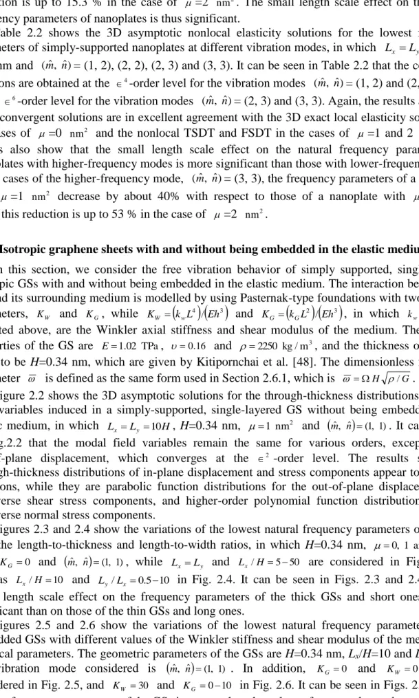
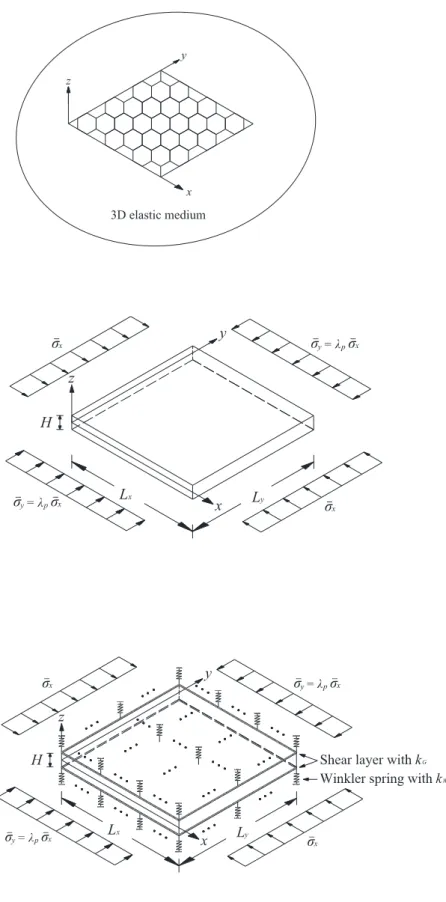
(12) Chapter 2 Free vibration analysis of embedded single-layered nanoplates and graphene sheets by using the multiple time scale method 2.1 Basic equations of 3D nonlocal elasticity theory As shown in Fig. 2.1, we consider a simply-supported, single-layered elastic nanoplate (or GS) surrounded by a Pasternak-type foundation and with the in-plane dimension Lx x Ly and total thickness H. A set of Cartesian coordinates ( x, y and z ) is located at the mid-plane of the plate. The main difference between the local and nonlocal elasticity theories is in their descriptions of the constitutive relation of a Hookean solid. In the former, the stress components induced at a particular material point of the deformed elastic body depend only on the strain components induced at that point, while in the latter, these will depend on the strain components induced at all the material points of the continuum, due to the small length scale effect. According to Eringen [41, 42] and Eringen and Edelen [43], the nonlocal constitutive behavior of an elastic body can be written as  ij x     x  x ,   Cijkl  kl xdV x,. x V ,. (2.1). in which Cijkl is the elastic modulus tensor of classical isotropic elasticity, and  ij and  kl are stress and strain tensors, respectively.   x  x ,   denotes the nonlocal modulus or attenuation function, which incorporates the constitutive equations into the nonlocal effect at the reference point x produced by local strain at the source x , and x  x is the Euclidean distance.   e0 a / l , in which e0 is a constant appropriate to each material, a is an internal characteristic length (e.g., length of C-C bond, lattice parameter, or granular distance), and l is an external characteristic length (e.g., crack length or wavelength). The value of e0 needs to be determined from experiments or by matching the dispersion curves of plane waves with those of atomic lattice dynamics [44]. The integral-partial differential equations of Eq. (2.1) can be further reduced to singular partial differential equations of a special class of physically admissible kernels, as follows:. 1     2. ij.  Cijkl  kl ,. (2.2). where  is the nonlocal parameter, and   e0 a 2 , and e0 a  2.0 nm for a single-walled CNT [45].  2 is the Laplacian operator, in which  2   xx   yy   zz  is used for a 3D nonlocal elastic problem, while  2   xx   yy  and 2   xx for the 2D and 1D nonlocal elastic ones, and  kk   2 /  k 2 (k  x, y and z) . According to Eringen’s elasticity theory, the linear constitutive equations valid for the symmetrical class of elastic materials are given by  x  c11 c12 c13 0 0 0    x        y  c12 c22 c23 0 0 0    y   z  c c c 0 0 0    z  1    2     13 23 33   ,  yz   0 0 0 c44 0 0   yz   xz   0 0 0 0 c55 0   xz        xy   0 0 0 0 0 c66   xy . . where. . x. . . x. . . denote the strain components.  lx ,  ly ,  zl ,  xzl ,  lyz ,  xyl  and are defined as the local and nonlocal stress components, respectively, in. ,  y ,  z ,  xz ,  yz ,  xy. ,  y ,  z , xz , yz , xy. (2.3). l   1    2  x ,  y ,  z , xz , yz , xy  . cij (i, j=1-6) are the elastic which  ,  ,  ,  ,  lyz ,  xy coefficients relative to the geometrical axes of the plate. For an isotropic material nanoplate the l x. l y. l z. l xz. 3.

(13) c11  c 22  c 33  1    E / 1   1  2  be reduced to , c12  c13  c 23   E / 1   1  2  and c 44  c 55  c 66   E / 2 1   , in which E and  are the Young’s modulus and Poisson’s ratio, respectively. The kinematic equations in terms of the Cartesian coordinates are. coefficients. will. cij.   x   x    0  y    z   0    yz   0  xz   z     xy   y. 0 0  u  z  x   u  , y y u x  z   0 . 0 y 0 z 0 x. (2.4). in which u x , u y and u z are the displacement components, and  k ,   /  k (k  x, y and z ) . The motion equations of an elastic body are given by  x  xy  xz  2u x    , x y z t2  xy x  x z x. .  y y. . .  yz y.  yz. . z. .  2u y t2.  z  2u z  z t2. (2.5). ,. (2.6) ,. (2.7). where  denotes the mass density of the nanoplate, and t is the time variable. The boundary conditions of the problem are specified as follows: On the top and bottom surfaces the transverse loads are given by. . xz.  yz. .  z  0. 0. q z. . on. z  h ,. (2.8). where h denotes one-half of the total thickness (H), the positive directions of q z and q z are defined to be upward and downward, respectively, q z  k w u z  k G u z , xx k G u z , yy and q z  k w u z  k G u z , xx k G u z , yy , in which k w and k G are the Winkler stiffness and the shear modulus of the surrounding elastic medium, respectively, and u z is the out-of-plane displacement at the mid-plane of the nanoplate/GS. The edge boundary conditions of the plate are considered as simply-supported ones, and are given as follows: At the edges ( x  0 and x  Lx ), the boundary conditions are x  u y  u z  0,. (2.9a). At the edges ( y  0 and y  Ly ), the boundary conditions are  y  u x  uz  0 .. (2.9b). 2.2 Nondimensionalization A set of dimensionless coordinates and elastic field variables is defined, as follows: x1  x / L, x 2  y / L, x 3  z / L  , u 1  u x /L , u 2  u y /L , u3 u z / L ,  1   x /Q ,  2   y /Q,  12   xy /Q , 2 2  13   x z / Q   ,  23   yz / Q  ,  3   z / Q 3  , 1   / L2 ,.  2   / L2 4  ,. (2.10a-n) 4.

(14) where  h / L . L and Q denote the reference length and elastic modulus, and these are given as L Lx L y and Q  E in this work, in which E is the Young’s modulus of the nanoplate. The dimensionless multiple time scales are defined as follows:  2 k  L . Q  t  0 . k . k  0, 1, 2, etc. ,. (2.11). in which  0 denotes a reference mass density, and this is taken to be  0   . As we previously listed in Eqs. (2.3)_(2.7), there are fifteen basic equations of 3D nonlocal elasticity theory for the free vibration analysis of nanoplates and GSs. In order to make the formulation suitable for mathematical treatment, we eliminate the in-plane stress (  x ,  y ,  x y ) and strain (  ,  ,  ,  ,  ,  ) components from Eqs. (2.3)_(2.7), introduce Eqs. (2.10) and (2.11) in x. y. z. xz. yz. xy. the resulting equations, and then express the 3D nonlocal equations in terms of the dimensionless forms of displacement ( u1 , u 2 , u 3 ) and transverse stress (  13 ,  23 ,  3 ) components, as follows: (2.12) u 3 , 3  2 L1 u 4 c~331 1  1  11  1  22  3  6 c~331  2  33  3 , u, 3   D u 3 2 S 1  1  11  1  22  s  4 S  2  33  s ,. (2.13). 1  1  11  1  22  s , 3  L 2 u  2  2  333  s  2 L 3 1  1  11  1 22  3  4 L 3  2  33  3  2  1 1  1  11  1 22   2   0  2   2  2 1  2  2   2  2  x3    0.      u (2.14)       2  2 2   2  4  2     u,         12   0 1  0 2    2  2  2   0  1.   4  .  2 2 2      12 0 2 . 1  1  11  1  22  3 , 3  DT  1  1  11  1  22   s   2   2 1  1  11  1  22   2 2  2    0. where u  u  1, u 2 .   D   1 ,  2 . L 3  LT1 ,. ~ l 31  c~13  1 ,. ~ ~ ~ l 52  Q66  11  Q22  22 ,. . Qij  cij  ci3 c j 3 / c33.  .  c~ 1 S   55  0. 0  , ~ c 441 .  . ~ l 32  c~23  2 , c~i 3  c i 3 / c 33.  i  1, 2 and 6 ,.  2 2    0 1 .   4  .  2 2 2      12 0 2 . .    s   13  ,  23 . and 2 ,. ~ l L 2  ~41  l42. ~  l42 ~ , l52 . . ~ ~ ~ l 42  Q12  Q66  12 ,. c~kk  c kk / Q. . ~ l32 ,. . ~ ~ ~ l 41  Q11  11  Q66  22 ,. i  1. . ~ L1  l31.  , (2.15)     u 3   . k  3  5 ,. ~ Qij  Qij / Q ,. . 1   / 0 and 2   / 0 2 .. Following a similar derivation process, we rewrite the in-plane stresses in the dimensionless form, as follows:. 1  1  11  1  22  p  B1 u  2   2  33  p  2 B 2 1  1  11  1  22  3  4 B 2  2  33  3 , where  1     p  2  ,    12 . ~ Q 11  1 ~ B 1   Q12  1 ~ Q  66  2. ~ Q12  2   ~ Q22  2  , ~ Q66  1 .  c~13  B 2  c~23  .  0 . 5. (2.16).

(15) The dimensionless forms of the boundary conditions of the problem are specified as follows: On the top and bottom surfaces the transverse loads are given by.  13.  23. in which q 3  q z.  / Q   .. 3 0. q 3. 0. . on. x 3  1 ,. (2.17). 3. At the edges ( x1  0 and x1  L x / L ), the boundary conditions are  1  u2  u3  0 ;. (2.18a). At the edges ( x2  0 and x2  Ly / L ), the boundary conditions are  2  u1  u3  0 .. (2.18b). 2.3 Asymptotic expansion By observation of Eqs. (2.12)-(2.16), we find that these contain terms involving only even powers of  . We thus asymptotically expand the field variables in the powers 2 , as given by f ( x1 , x 2 , x3 , t )  f (0) ( x1 , x 2 , x3 ,  0 ,  1 , ) 2 f (1) ( x1 , x 2 , x3 ,  0 ,  1 , ) 4 f ( 2) ( x1 , x 2 , x3 ,  0 ,  1 , )   .(2.19). Substituting Eq. (19) into Eqs. (2.12)-(2.16) and collecting coefficients of equal powers of  , we obtain the following sets of recurrence equations. Order 0 : u (30) , 3  0 ,. (2.20). u ( 0) , 3 D u (30) ,. (2.21). 1  . 1. 1  . (0) , 3   D T 1   1  11   1  22  s( 0 )   2 1   1  11   1  22  1  11   1  22  3. .  11  1  22   s( 0) , 3  L 2 u ( 0)   1 1  1  11  1  22 . . .  2 u ( 0)  02. ,. . (2.22)  2 u 3( 0 )  02. ,. 1  1  11  1  22  (p0)  B1 u (0) ,. (2.23) (2.24). Order 2 k (k=1, 2, 3,... ):. . . u 3( k ) , 3  L 1 u ( k 1)  c~331 1  1  11  1  22  (3k  2)  c~331  2  33  (3k 3) ,. (2.25). u ( k ) , 3   D u (3k )  S 1  1  11  1  22  (sk 1)  S  2  33  (sk  2) ,. (2.26). 1  . 1. .  11  1  22  (sk ) , 3  L 2 u ( k )   2  333  (sk 1) L 3 1  1  11  1  22  (3k 1)  L 3  2  33  (3k  2 )   2 u (k )  2 u ( k 1)  2 2 2   1 1  1  11  1  22    2   2  0  1   0  2  12   0   2    2 u ( k 1)   2 u ( k  2)   1  2  2    2  , 2  0  1   x 3    0. 1  . 1. . .  11  1  22  (3k ) , 3  D T 1  1  11  1  22  s( k )  u   2 1  1  11  1  22     2. (k ) 3 2 0. 2. .   u 2 2   2   0  1   0  2  12 2.   ( k  2) u   , (2.27)   . ( k 1) 3.  (2.28)  ( k  2)  u3  ,   . 1  1 11  1  22  (pk )  B1 u(k )   2 33   (pk 1)  B2 1  1 11  1  22  (3k 1)  B2 233  (3k  2) . 6. (2.29).

(16) The boundary conditions for various order problems are specified, as follows: On the top and bottom surfaces the transverse loads are Order 0 ,. . ( 0)  23. ( 0) 13. q .  (0) 3. where. . K w  k w L4 / Qh 3. . .  (30)  0. 0. q .  ( 0) 3.  2 2   K w u 30  K G  2  2  x1 x 2.  . . and K G  k G L2 / Qh 3  .. Order 2 k (k =1, 2, 3, etc),. . (k )  23. (k ) 13. . . .  (3k )  0. 0. q .  (k ) 3.  2 2  2 2  x1 x 2.  0  u3  .  . .  k  u3  . where q 3    K w u 3k   K G  (k ). on.  . x3  1 ,. q . (2.30a).  (0) 3. and.  2 2  K w u 30  K G  2  2  x1 x 2.  .  0  u3  .  . x3  1 ,. on. ,. and. (2.30b)  2 2  2 2  x1 x 2. and q 3   K w u 3k   K G  (k ).  k  u3  .  .. Along the edges ( x1  0 and x1  L x / L ), the boundary conditions are given, as follows: order 2 k (k =0, 1, 2, 3, etc),  (1k )  u (2k )  u (3k )  0 ;. (2.31a). Along the edges ( x2  0 and x2  Ly / L ), the boundary conditions are given as follows: order 2 k (k =0, 1, 2, 3, etc),  (2k )  u (1k )  u (3k )  0 .. (2.31b). 2.4 Asymptotic integration and various order problems 2.4.1 The ∈𝟎 -order problem We examine the sets of asymptotic equations and find that the present analysis can be carried out by integrating these through the thickness direction. We thus integrate Eqs. (2.20) and (2.21) to obtain u (30)  u 03 ( x1 , x 2 ,  0 ,  1 ,  ) ,. (2.32). u (0)  u 0  x 3 D u 03 ,. (2.33). where u 03 and u0  u01( x1, x2 , 0 ,1,) u02 ( x1, x2 , 0 ,1,) represent the displacement components on the mid-plane, and these are also of the Kirchhoff-Love type in CPT. With the boundary conditions on x3=-1 given in Eq. (2.30a), we then proceed to integrate Eqs. (2.22) and (2.23), which yields T. 1  1 11  1 22  s(0) 1. x3. . . L u 2. 0. .   D u 03 d  1  1  11  1  22 . . x3. 1. 1. . . 2 u 0   D u 03 d ,  02. 1  1  11  1  22   (30)  q 3 (0)  1 ( x3  ) DT L 2 u 0   D u 03  d  1  1  11  1  22 1  2 x3. x3. .  2 u 03  02. d. . 2  1  1  11  1  22  1 ( x 3   ) D u 0   D u 03 d , 2 1  0 x3. 7. T. (2.34). (2.35).

(17) Imposing the remaining lateral boundary conditions on x3=1 given in Eq. (2.30a) in Eqs. (2.34) and (2.35), we obtain   3 u 30  2 u10 K 11 u 01  K 12 u 02  K 13 u 03  1  1  11  1  22   I 10  I 11  02 x1  02 .  ,  . (2.36).   3 u 30  2 u 20 K 21 u 01  K 22 u 02  K 23 u 03  1  1  11  1  22   I 10  I 11  02 x 2  02 .  ,  . (2.37).   4 u 30  4 u 30  2 u 30  3 u10  3 u 20 * K 31 u 01  K 32 u 02  K 33  K 33 u 03  1  1  11  1  22   I 11  I  I  I  I 11 12 12 20 2 x 2  02 x12  02 x 22  02  02  x1  0. . where. . ~ ~ K11   A11 11  A66  22. . . K 31   K 13 ,. . . . . ~ ~ ~ ~ K33  D11 1111  2D12  4D66 1122  D22  2222 ,. K 32   K 23 ,. ~ * K33  1  111  122  2Kw  2KG 11  22  , Aij  ~ Dij . . 1. 1. ~ x32 Qij dx3 , I kl . . 1. 1. . ~ ~ ~ K13  B11 111  B12  2B66  122 ,. ~ ~ ~ K 23  B12  2B66 112  B22  222 ,. ~ ~ K 22   A66  11  A22  22 ,. K 21  K 12 ,. . ~ ~ K12   A12  A66  12 ,. ,.   , (2.38)  . . 1. 1. ~ Qij dx3 ,. ~ Bij . . 1. 1. ~ x3 Qij dz,.  k x3 l dx3 .. (2.39a-n). In this paper, the edge boundary conditions of the plate are considered as fully simply-supported edges. After the asymptotic process, we thus obtain the edge conditions for the leading order problem, as follows: u 20  0 ,. u 30  0 ,. N (0) 1  0. and. M (0) 1 0,. at x1  0 and x1  L x / L ,. (2.40a). u10  0 ,. u 30  0 ,. N (0) 2  0. and. M (0) 2 0,. at x 2  0 and x2  L y / L ,. (2.40b). 1. 1. in which N (0)i  1  (i0) dx3 , M (0)i  1 x3  (i0) dx3 , and i=1 and 2. It is noted that Eqs. (2.36)-(2.38) are exactly the same as the motion equations of the nonlocal CPT, which have thus been derived as a first-order approximation of the 3D nonlocal elasticity theory. The solutions of Eqs. (2.36)-(2.38) must be supplemented with the edge boundary conditions given in Eqs. (2.40a) and (2.40b) to constitute a well-posed boundary value problem. Once the modal variables of u 01 , u 02 and u 03 are determined, the leading-order solutions of modal displacements are given by Eqs. (2.32) and (2.33), the modal transverse shear and normal stresses by Eqs. (2.34) and (2.35) and the in-plane stresses by Eq. (2.24). 2.4.2 The ∈𝟐 -order problem Proceeding to order 2 and following the same process as before, we readily obtain u (31)  u 13 x1 , x 2 ,  0 ,  1 ,    31 x1 , x 2 , x 3 ,  0 ,  1 ,  ,. (2.41). u (1)  u 1 x1 , x 2 ,  0 ,  1 ,   x 3 D u 13   1 x1 , x 2 , x 3 ,  0 ,  1 ,  ,. (2.42). 1  1  11  1  22  s(1).  . x3. 1. L u   D u  d  f 1. 2. 1 3. 1. x1 , x 2 , x3 ,  0 ,  1 , .  1  1  11  1  22    1 x3. 1. 8. . . 2 u 1   D u 31 d ,  02. (2.43).

(18) . . 1  1  11  1  22   (31)  q 3 (1)  1 ( x3   ) D T L 2 u1   D u 13  d  f 31 x1 , x3. x3.  2 u 31. 1.  02.  1  1  11  1  22   2. x 2 , x 3 ,  0 ,  1 , . d. (2.44).  1  1  11  1  22   1 ( x 3   ) D T x3. 1. where. . u1  u11 ( x1, x2 , 0 ,1,). . . 2 1 u   D u 13 d , 2  0. . T. u12 ( x1, x2  0 ,1,) ,. 31 ( x1, x2 , x3 , 0 ,1,)    L1u( 0) d , x3. 0. x  ( x , x , x , , ,) (0)  1   11 1 2, 3 0 1   1  1 11  1  22   0 S  s  D31 d ,  ( x , x , x ,  ,  ,  )  21 1 2 3 0 1  3. . . x3  f x , x , x , , , f 1   11 1 2 3 0 1    L 2  1  2  333  s( 0)  L3 1  1 11  1  22  (30) d  1  f 21 x1 , x2 , x3 , 0 , 1 ,  x3   2 1  2u ( 0 )   2   2u( 0)    2 2   d ,   1  1  1 11  1  22  2  2  1  0 1  x3   02     0. . f 31 x1 , x2 , x3   . . x3. 1. . DT f 1 d  1  111  1 22 . . x3. 1.   2u3( 0)  231   d .  2  2  2    0 1  0 . and u 1 represent the 2 -order modifications to the modal displacement components. By imposing the associated lateral boundary conditions (Eq. (2.30b)) on Eqs. (2.43) and (2.44), we again obtain the motion equations of nonlocal CPT, and the nonhomogeneous terms can be calculated using the lower-order solution. The resulting equations are obtained, as follows: u 13.   3 u 31  2 u11 K 11 u 11  K 12 u 12  K 13 u 13  1  1  11  1  22   I 10  I 11 2  0 x1  02 .    f 11 x 3  1 ,  .   3 u 31  2 u 12 K 21 u 11  K 22 u 12  K 23 u 13  1  1  11  1  22   I 10  I 11  02 x 2  02 .    f 21 x 3  1 ,  . (2.45) (2.46).   4 u 31  4 u 31  2 u 31  3 u11  3 u 12 * K 31 u11  K 32 u 12  K 33  K 33 u 31  1  1  11  1  22   I 11  I  I  I  I 11 12 12 20 2 x 2  02 x12  02 x 22  02  02  x1  0 f ( x  1) f 21 ( x 3  1)  f 31 x 3  1  11 3  . x1 x 2. . .     (2.47). After the asymptotic process, we obtain the edge conditions for the higher-order problems, as follows: u 12  0 ,. u 31  0 ,. N (1) 1  0. and. M (1) 1 0,. at x1  0 and x1  L x / L ,. (2.48a). u11  0 ,. u 31  0 ,. N (1) 2  0. and. M (1) 2 0,. at x 2  0 and x2  L y / L ,. (2.48b). 1. 1. in which N (1)i  1  (i1) dx3 , M (1)i  1 x 3  (i1) dx3 , and i=1 and 2. The 2 -order modifications of mid-plane displacement components ( u11 , u 12 and u 31 ) can be obtained by solving Eqs. (2.45)-(2.47) combined with the edge conditions given in Eqs. (2.48a) and (2.48b). Once these are determined, the 2 -order modifications of modal displacement components. 9.

(19) are given by Eqs. (2.41) and (2.42), the transverse stresses by Eqs. (2.43) and (2.44) and the in-plane stresses by Eq. (2.29). Equations (2.36)-(2.38) and (2.45)-(2.47) show that the differential operators among the various order problems remain identical, and the nonhomogeneous terms of higher-order problems can be calculated from the lower-order solution. The solution process of the leading-order problem can be repeatedly applied to the higher-order problems. The present asymptotic solutions can thus be determined order-by-order in a hierarchical and consistent manner. 2.5 Applications 2.5.1 ∈𝟎 -order solution The free vibration problem of simply-supported, single-layered nanoplates and graphene sheets embedded in the elastic medium is studied using the Eringen nonlocal elasticity theory and multiple time scale method, in which the primary variables of displacement, and local and nonlocal stress components are expanded as the double Fourier series functions in the in-plane coordinates, such that the simply-supported boundary conditions are satisfied. The motion equations of the 0 -order problem can thus be solved by letting . u10 x1 , x 2 , 0 , 1 ,   . . ~x sin n ~x cos      , u 01mˆ nˆ cos m 1 2 0 . . (2.49). ˆ 1 nˆ 1 m . u 02 x1 , x 2 , 0 , 1 ,    ˆ 1 m. . u 03 x1 , x 2 , 0 , 1 ,    ˆ 1 m. ~  mˆ  L / L m x. where. . u. 0 ˆ nˆ 2m. ~x cos n ~x cos     , sin n 1 2 0 . (2.50). 0 ˆ nˆ 3m. ~ x sin n ~x cos     , sin m 1 2 0 . (2.51). nˆ 1. . u nˆ 1. ~  nˆ  L / L , n y. ,. mˆ. and nˆ. . are the positive integers.. denotesthe. dimensionless natural frequency of the nanoplate, and the dimension one is    Q /  0 / L .   denotes the phase angle,       1 ,  2 ,  , and for brevity the summation sign will not be shown in the following derivation. Substituting Eqs. (2.49)-(2.51) into Eqs. (2.36)-(2.38) gives   k11   k 21   k 31. k12 k 22 k 32. k13 k 23 * k 33  k 33. .     2 1  m ~ 2  n~ 2 1  . . . . .  I 10  0  ~I  m 11. ~I m 11  n~ I 11 ~ 2 I  n~ 2 I  I m 12 12 20. 0 I 10  n~ I 11. . 0   u1mˆ nˆ  0    u 0  0 , (2.52)    2 mˆ nˆ       u 30mˆ nˆ     0. . ~ 2 A  n~ 2 A , k  m ~ n~ A  A  , k  m ~3B  m ~n ~ 2 B  2B  , where k11  m 11 66 12 12 66 13 11 12 66 ~. k 21  k 12 ,. ~. ~. ~. ~. . ~. . ~ ~ ~ 2n ~ B ~3 ~ k 23  m 12  2 B66  n B22 ,. ~ ~2 A ~2 ~ k 22  m 66  n A22 ,. . ~. . ~ ~ ~4 D ~ 2 ~2 ~ ~4 ~ k33  m 11  m n 2D12  4D66  n D22 ,. . . . k 32  k 23 ,. k 31  k 13 ,. . . * ~ 2  n~ 2 2K  2K m ~ 2  n~ 2 . k33  1  1 m w G. The motion equations (2.52) represent a standard eigen-valued problem. A nontrivial solution of Eq. (2.52) exists if the determinant of the coefficient matrix vanishes:. . . . ~ 2  n~ 2 I k11   2 1  1 m 10 k 21 ~ 2  n~ 2 m ~I  k 31   2 1  1 m 11. . . . k12 2 ~ 2  n~ 2 I k 22   1  1 m 10 ~ 2  n~ 2 n~ I  k 32   2 1  1 m 11. . . . . . .  .  .  . ~ 2  n~ 2 m ~I  k13   2 1  1 m 11 ~ 2  n~ 2 n~ I  k 23   2 1  1 m  0 , (2.53) 11 * 2 2 2 2 2 ~ ~ ~ ~ k 33  k 33   1  1 m  n m I 12  n I 12  I 20. . . . . . . From this, three eigenvalues  i i  1 3 that represent the 0 -order natural frequencies for a fixed values of mˆ and nˆ are obtained. 10.

(20) To make the solution unique, the modal displacement components are normalized by imposing the normality condition:. u. 0 1mˆ nˆ.  .  . 2. . 2.  2 u11mˆ nˆ  4 u12mˆ nˆ    u 20mˆ nˆ  2 u 12 mˆ nˆ  4 u 22mˆ nˆ    u 30mˆ nˆ  2 u 31mˆ nˆ  4 u 32mˆ nˆ  . 2. 1.. (2.54). The normality conditions at each level are 0 -order:. u   u   u .  2 -order:. u. 0 ˆ nˆ 1m. u11mˆ nˆ  u 20mˆ nˆ u 12mˆ nˆ  u 30mˆ nˆ u 31mˆ nˆ  0 ,.  4 -order:. u. 0 1mˆ nˆ. u12mˆ nˆ  u 20mˆ nˆ u 22mˆ nˆ  u 30mˆ nˆ u 32mˆ nˆ   1 / 2  u11mˆ nˆ. 2 0 1mˆ nˆ. 2 0 2 mˆ nˆ. 2 0 3 mˆ nˆ. 1 ,. (2.55a). . . (2.55b). .   u   u  , etc. 2. 2 1 2 mˆ nˆ. 2 1 3 mˆ nˆ. (2.55c). Once the natural frequencies of the 0 -order problem (  i , i=1-3) are obtained, the corresponding eigen vectors, which are the modal mid-plane displacement components, can be uniquely determined by using the corresponding normality conditions (Eqs. (2.55a)-(2.55b)), and the through-thickness distributions of modal displacement and stress variables for the 0 -order problem can thus be determined, as mentioned before. 2.5.2 First-order modifications Carrying on the solution to order 2 , we find that the nonhomogeneous terms ( f i1 x1 , x 2 , 1,  0 ,  1 , , i  1  3 ) and the revelant functions (  i1 x1 , x 2 , x3 ,  0 ,  1 ,  (i=1-3)) for fixed values of mˆ and nˆ in the 2 -order equations are ~ x sin n~x cos      , f 11 ( x1 , x 2 , 1,  0 ,  1 , )  f 11mˆ nˆ 1 cos m (2.56) 1 2 0 . and. ~ x cos n~x cos      , f 21 ( x1 , x 2 , 1,  0 ,  1 , )  f 21mˆ nˆ 1 sin m 1 2 0 . (2.57). ~ x sin n~x cos      , f 31 ( x1 , x 2 , 1,  0 ,  1 , )  f 31mˆ nˆ 1 sin m 1 2 0 . (2.58). ~ x sin n~x cos      , 11 ( x1 , x 2 , x 3 ,  0 ,  1 , )  11mˆ nˆ cos m 1 2 0 . (2.59). ~ x cos n~x cos      ,  21 ( x1 , x 2 , x 3 ,  0 ,  1 , )   21mˆ nˆ sin m 1 2 0 . (2.60). ~ x sin n~x cos      ,  31 ( x1 , x 2 , x 3 ,  0 ,  1 , )   31mˆ nˆ sin m 1 2 0 . (2.61). where, f 11mˆ nˆ , f 21mˆ nˆ , f 31mˆ nˆ and 11mˆ nˆ ,  21mˆ nˆ ,  31mˆ nˆ are the relevant coefficients. In view of the recurrence of the equations, the 2 -order solution can be obtained by letting ~x sin n~x cos      , u11 x1 , x 2 ,  0 ,  1 ,   u11mˆ nˆ cos m 1 2 0 . (2.62). ~x cos n~x cos      , u 12 x1 , x 2 ,  0 ,  1 ,   u 12mˆ nˆ sin m 1 2 0 . (2.63). ~x sin n~x cos      . u 31 x1 , x 2 ,  0 ,  1 ,   u 31mˆ nˆ sin m 1 2 0 . (2.64). Substituting Eqs. (2.56)-(2.64) into Eqs. (2.45)-(2.47) gives   k11 k12   k 21 k 22   k 31 k 32. k13 k 23 * k 33  k 33. .     2 1  m ~ 2  n~ 2 1  . . . . .  I 10  0  ~I  m 11. 0 I 10  n~ I 11. ~I m 11  n~ I 11 ~ 2 I  n~ 2 I  I m 12 12 20. . ~      ˆ  f 11mˆ nˆ 1   f 11mˆ nˆ 1   0   1     u1mˆ nˆ      u 0    ~f 1      fˆ 1  , (2.65)    21mˆ nˆ     2 mˆ nˆ   21mˆ nˆ  1    u 30mˆ nˆ            ~  gˆ 31mˆ nˆ 1   g 31mˆ nˆ 1       1 . . ~ ~ ~~ ~ fˆ 1  n~ fˆ 1 , and in which g~31mˆ nˆ 1  f 31mˆ nˆ 1  m f 11mˆ nˆ 1  n~ f 21mˆ nˆ 1 , gˆ 31mˆ nˆ 1  fˆ31mˆ nˆ 1  m ˆ nˆ 11m 21mˆ nˆ.    1 ,  2 ,    1  1    ( 2)  2 ,  3 ,  . 11.

(21) A solvability condition for a particular vibration mode (i), the natural frequency of which is i , is introduced such that Eq. (2.65) becomes solvable, and this is given by. u. 0 1mˆ nˆ. u20mˆ nˆ. u30mˆ nˆ.  i.     ~   f11mˆ nˆ 1     1  .   ˆ  f11mˆ nˆ 1  . ~    f 21mˆ nˆ 1     1.   ˆ  f 21mˆ nˆ 1  . ~    g31mˆ nˆ 1     1. T.     gˆ 31mˆ nˆ 1   0 .(2.66)    i. Equation (2.66) leads to       1.  . .  (2.67).  ~ ~ 0 0 0 ~ ˆ ˆ    u10mˆ nˆ f 11mˆ nˆ 1  u 20mˆ nˆ f 21mˆ nˆ 1  u 30mˆ nˆ g ˆ 31mˆ nˆ 1 ˆ nˆ 1 i / u1m ˆ nˆ f 11m ˆ nˆ 1  u 2 m ˆ nˆ f 21m ˆ nˆ 1  u 3m ˆ nˆ g 31m i.  . i.   1 i .. The hamonic time function can then be modified as.      cos      h / L      ,  . cos  i  0    i   cos  i  0  1 i  1   ( 2)  2 ,  3 ,  i 2. 1. i. ( 2). 0. i. . 2. 3. . ,  i ,. (2.68). and the natural frequencies for the first-order problem are thus obtained as.         h / L  (1). 1. i. i. i. 2. .. (2.69). By using the solvability conditions (2.66) and the normality conditions (2.54), we can uniquely determine the first-order modifications of interlaminar modal displacement and stress components for the ith vibration mode. Moreover, the solution process can be repeatedly applied to higher-order problems ( 2 k -order, k=2, 3, etc) in a systematic and consistent manner due to the similarity between the system equations of the first-order problem (k=1) and those of much higher-order ones (k=2, 3, etc.). 2.6 Illustrative examples 2.6.1 Isotropic nanoplates The free vibration problem of simply supported, single-layered isotropic plates without being embedded in the elastic medium, has been studied by Aghababaei and Reddy [46] using the nonlocal third-order shear deformation theory (TSDT), FSDT and CPT. These solutions are used to validate the performance of the 3D asymptotic nonlocal elasticity theory. The geometric parameters of the nanoplate are given as Lx=10 nm, Ly/Lx=1 and 2, and Lx/H=10 and 20, and the material properties of this are E=3x107,   0.3 and   1 , the units of which were not given in the earlier work [47] because the natural frequencies of the plate were expressed as a dimensionless form,    H  / G , in which G is the shear modulus of the nanoplate and G  E /2 1    . Table 2.1 shows results of the convergence study with regard to the 3D asymptotic nonlocal elasticity solutions for the lowest frequency parameters of the nanoplate, in which the nonlocal parameter  was taken to be  =0, 1 and 2 nm 2 . When  =0 nm 2 , the results of nonlocal theory will be reduced to those of local theory. It can be seen in Table 1 that the asymptotic solutions converge rapidly. For a moderately thick isotropic nonlocal plate (Lx/H=10), the convergent solutions are obtained at the 2 -order level, and these are in excellent agreement with the local 3D exact solutions in the cases of  =0 nm 2 and the nonlocal TSDT and FSDT in the cases of  =1 and 2 nm 2 . The results also show the natural frequency parameters decrease when the nonlocal parameter becomes greater, which means the small length scales will soften the nanoplate. For a moderately thick isotropic nonlocal plate (Lx/H=10), the frequency parameters of a nanoplate with  =1 nm 2 decrease by about 8.6% with respect to those of a macroplate (  =0 nm 2 ), while this. 12.

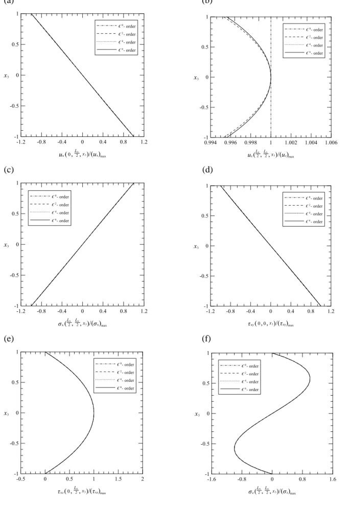
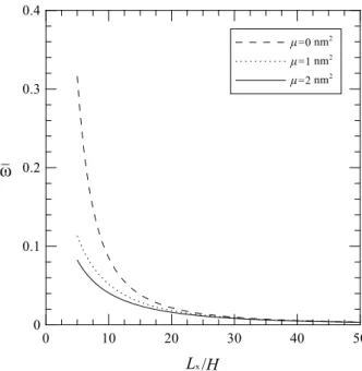
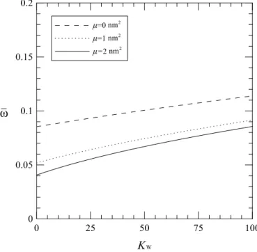
(22) reduction is up to 15.3 % in the case of  =2 nm 2 . The small length scale effect on the natural frequency parameters of nanoplates is thus significant. Table 2.2 shows the 3D asymptotic nonlocal elasticity solutions for the lowest frequency parameters of simply-supported nanoplates at different vibration modes, in which Lx  L y  10 nm , H=1 nm and ( mˆ , nˆ ) = (1, 2), (2, 2), (2, 3) and (3, 3). It can be seen in Table 2.2 that the convergent solutions are obtained at the 4 -order level for the vibration modes ( mˆ , nˆ ) = (1, 2) and (2, 2), while at the 6 -order level for the vibration modes ( mˆ , nˆ ) = (2, 3) and (3, 3). Again, the results also show these convergent solutions are in excellent agreement with the 3D exact local elasticity solutions in the cases of  =0 nm 2 and the nonlocal TSDT and FSDT in the cases of  =1 and 2 nm 2 . The results also show that the small length scale effect on the natural frequency parameters of nanoplates with higher-frequency modes is more significant than those with lower-frequency modes. In the cases of the higher-frequency mode, ( mˆ , nˆ ) = (3, 3), the frequency parameters of a nanoplate with  =1 nm 2 decrease by about 40% with respect to those of a nanoplate with  =0 nm 2 , while this reduction is up to 53 % in the case of  =2 nm 2 . 2.6.2 Isotropic graphene sheets with and without being embedded in the elastic medium In this section, we consider the free vibration behavior of simply supported, single-layered isotropic GSs with and without being embedded in the elastic medium. The interaction between the GS and its surrounding medium is modelled by using Pasternak-type foundations with two stiffness parameters, K W and K G , while KW  k w L4  / Eh 3  and K G  k G L2  / Eh 3  , in which k w and k G , as noted above, are the Winkler axial stiffness and shear modulus of the medium. The material properties of the GS are E  1.02 TPa ,   0.16 and   2250 kg / m 3 , and the thickness of GSs are fixed to be H=0.34 nm, which are given by Kitipornchai et al. [48]. The dimensionless frequency parameter  is defined as the same form used in Section 2.6.1, which is    H  / G . Figure 2.2 shows the 3D asymptotic solutions for the through-thickness distributions of modal field variables induced in a simply-supported, single-layered GS without being embedded in the elastic medium, in which Lx  L y  10 H , H=0.34 nm,   1 nm2 and mˆ , nˆ   (1, 1) . It can be seen in Fig.2.2 that the modal field variables remain the same for various orders, except for the out-of-plane displacement, which converges at the 2 -order level. The results show the through-thickness distributions of in-plane displacement and stress components appear to be linear functions, while they are parabolic function distributions for the out-of-plane displacement and transverse shear stress components, and higher-order polynomial function distributions for the transverse normal stress components. Figures 2.3 and 2.4 show the variations of the lowest natural frequency parameters of the GSs with the length-to-thickness and length-to-width ratios, in which H=0.34 nm,   0, 1 and 2 nm2 , K W  K G  0 and mˆ , nˆ   (1, 1) , while Lx  L y and L x / H  5  50 are considered in Fig. 2.3, as well as L x / H  10 and L y / Lx  0.5 10 in Fig. 2.4. It can be seen in Figs. 2.3 and 2.4 that the small length scale effect on the frequency parameters of the thick GSs and short ones is more significant than on those of the thin GSs and long ones. Figures 2.5 and 2.6 show the variations of the lowest natural frequency parameters of the embedded GSs with different values of the Winkler stiffness and shear modulus of the medium and nonlocal parameters. The geometric parameters of the GSs are H=0.34 nm, Lx/H=10 and Lx=Ly, and the vibration mode considered is mˆ , nˆ   (1, 1) . In addition, K G  0 and K W  0  100 are considered in Fig. 2.5, and K W  30 and K G  0  10 in Fig. 2.6. It can be seen in Figs. 2.5 and 2.6 that the frequency parameters of the GSs increase when the values of K W and K G become greater, and the increase trend seems to follow a monotonic linear function. 13.

(23) Table 2.1 Results of the convergence study with regard to the 3D asymptotic nonlocal elasticity solutions for the lowest frequency parameters (  ) of simply-supported nanoplates at vibration mode mˆ , nˆ   1, 1 , and without foundation models (Lx=10 nm). Ly/Lx=1. Ly/Lx=2. Lx/h=10. Lx/h=20. Lx/h=10. Lx/h=20. Theories   0 nm 2.   1 nm2.   2 nm 2.   0 nm 2.   1 nm2.   2 nm 2.   0 nm 2.   1 nm2.   2 nm 2.   0 nm 2.   1 nm2.   2 nm 2. Present 0. 0.0955. 0.0873. 0.0809. 0.0240. 0.0220. 0.0203. 0.0599. 0.0565. 0.0536. 0.0150. 0.0142. 0.0135. Present 2. 0.0931. 0.0850. 0.0788. 0.0239. 0.0218. 0.0202. 0.0589. 0.0556. 0.0528. 0.0150. 0.0141. 0.0134. Present 4. 0.0931. 0.0851. 0.0789. 0.0239. 0.0218. 0.0202. 0.0589. 0.0556. 0.0528. 0.0150. 0.0141. 0.0134. Present 6. 0.0931. 0.0851. 0.0789. 0.0239. 0.0218. 0.0202. 0.0589. 0.0556. 0.0528. 0.0150. 0.0141. 0.0134. Nonlocal CPT [46]. 0.0963 (0.0955). 0.0880. 0.0816. 0.0241. 0.0220. 0.0204. 0.0602. 0.0568. 0.0539. 0.0150. 0.0142. 0.0135. Nonlocal FSDT [46]. 0.0930 (0.0930). 0.0850. 0.0788. 0.0239. 0.0218. 0.0202. 0.0589. 0.0556. 0.0527. 0.0150. 0.0141. 0.0134. Nonlocal TSDT [46]. 0.0935 (0.0931). 0.0854. 0.0791. 0.0239. 0.0218. 0.0202. 0.0591. 0.0557. 0.0529. 0.0150. 0.0141. 0.0134. Local 3D exact [47]. 0.0932. NA. NA. NA. NA. NA. NA. NA. NA. NA. NA. NA. The solutions in parentheses for the nonlocal CPT, FSDT and TSDT denote natural frequency parameters obtained by Reddy and Phan [49], in which the rotary inertia effect is considered.. 15.