國立臺灣大學電機資訊學院電機工程學系 碩士論文
Department of Electrical Engineering
College of Electrical Engineering and Computer Science National Taiwan University
Master Thesis
運用 7 軸 3D 測量機台對複雜工件之精準量測及驗證 3D Coordinate Measurement Machine with 7-DoF Configuration
for Precise On-Machine Inspection and Validation of Complex Curvature Workpieces
李晟 Cheng Li
指導教授:羅仁權 博士
Advisor: Ren.C. Luo, Ph.D
誌謝
碩士班生涯是我嘗試研究生活的一段美好回憶。感謝父母親辛苦的栽培 與教誨,家人們給予我支持與鼓勵,讓我能夠全心全意接受挑戰,專心於我喜愛 的領域中。非常感謝我最敬愛的指導老師羅仁權教授,提供我們豐富的資源,讓 我可以親手打造理想中的機器人。從理念發想、設計、實驗、直到最後的成果展 現,無論在哪個環節都是一生難得的體驗,我也從中學到非常多寶貴的知識與經 驗。這一切都要感謝老師對我的指導及信任。兩年的師生互動中,老師充分展現 出國際級學者的視野與風範,不僅帶領我們探索學術知識的廣度與深度,更是給 予我們充分的機會去體驗本科系以外的經驗,希望我們成為均衡發展的人才。在 待人處事方面,老師更是諄諄教誨,提醒我們許多社會上應對進退的準則。這一 切都使我獲益良多,也確立我對於機器人領域的研究興趣,並決心朝此方向繼續 努力。此外,我想特別感謝研究所時期教導過我的黃漢邦老師與陳明新老師,是 他們為我打下機器人與控制理論的研究基礎,我從他們的課程中得到很多啟發。
研究生活中,感謝鐿文、陞佑、瑋隆、金成、献章、繼棠、昕昳、玲盈、志遠、
東榕、正倫等博班學長姊,還有智賢、士紘、柏宏、邦甫、冠志、建偉、文謙、金博、
耕銘、銘駿、煒森、建安等碩班學長姊,以及同屆的同學師兄俊豪、莉彤、長鈞、晴 岡、靖霖、昱佑、達方、凱鈞、仲凱、柏凱,最後還有積極認真又可愛的學弟妹們:
培淳、石崴、武昱、嵩詠、智堅、威辰、錦賢、育榕、育澤、名彥、展嘉、何鑫、曾旻、
王昊,謝謝大家給我的幫助,在研究上面一起討論,同甘共苦的參加比賽,一起幫
忙大大小小的事務,一起打球運動,這段時間真的很開心能夠跟大家一起經歷這 麼多事情,相信這都是令人印象深刻的生活點滴。也很感謝助理群們,有你們幫 忙處理繁瑣的事務,我們才能快速了解實驗室的情況,更專注於研究上。另外也
中文摘要
近年來,CNC robot 不斷推陳出新,其功用之廣泛且穩定已使其成為在眾多機 器人中成為相當具有潛力的一種,然而在一系列加工流程中,量測為一核心且極 具影響力的項目,在許多在精度方面要求甚高的工業中,量測為期提供了品質保 證、誤差判定的功效,如在航太業上,飛機機翼是一精度要求極高的大型加工件,
且其獨特的設計考量了氣流、風力、風阻等多項因素,一點點加工上的誤差便會 改變飛機在空中的穩定性,直接影響了上百人的安全,在小型加工件方面,如齒 輪,些微的誤差都會容易造成齒輪旋轉過程中卡住,破壞機械結構使整台機器故 障甚至報廢,由已上便可知道量測在加工中是如此重要。此篇碩論提出一就由裝 置高精度探針的多軸量測機來玩成對複雜曲面之量測。
多自由度之測量機台搭配冗餘度的特性後可在空間中有著相當大的工作範圍 及自由性,其末端點可以在位置不動的情況下改變旋轉以此來確定末端點之探針 探測工件表面的的點做量測時可以保證其以法向量觸碰,藉此得到準確的量測數 據,大多數的測量機台由於沒有多自由度之特性,常常在以非法向量的方式量測 後再額外進行計算出真正的觸碰點位置,此方法的缺點為由於無法真正準確地知 道觸碰點與探針末端點的關係,導致難以準確補償物差造成精確度下降。而在量 測技術方面,對於ㄧ有複雜曲面之工件的量測往往會由於缺乏參考點而無法找出 量測點,此篇碩論中一提出一針對複雜曲面之量測流程,其包括之內容有物件定 位、探針半徑補償、曲面量測點取樣、曲面重建、誤差分析及曲面精度分析等。
關鍵字: CNC 加工機、量測系統、曲面量測、探針、量測機台
ABSTRACT
For these years, CNC(Computer Numerical Control) machine has been developed at an incredibly high speed. Because of its high stability and wide applicability, this kind of machine is considered as the most powerful potential in the future development. In the series of machining procedure, measurement is a core and certainly influential item.
For many industries which require extremely high precision of a workpiece, measurement provides the insurance of quality and error decision for each workpiece.
Take aerospace industry for example, the airfoil is a large machined part which requires extremely high precision, which is specially designed that considers a lot of factors such as air flow, air mechanics, windage, and so on. Any small error may incredibly influence the characteristics above and decrease the flying stability. Another great example is gear.
Stuck is happened while the precision cannot be promised, which may furthermore destroy the whole equipment. This paper proposed a method for measuring a complex surface by a precise probing system mounted on the end-effector of measurement machine with high DoF.
For some measuring strategy, they use different sides of the end-effector to measure the points because of the limitation of lower degree of freedom. The merit of the strategy is effectively reflected on lower cost of hardware. However, the difficulty is increased because extra computation is needed for points with inaccessible orientation
algorithm is implemented on a 7-DoF measurement machine. Thanks to high reliability and high degree of freedom, the machine has extremely wide workspace and a redundant angle to make the end-effector can reach the target even an obstacle exists that may disturb the path of the manipulator. In the measurement technique aspect, a series of measurement procedure will be introduced and explained, including workpiece localization, probe radius compensation, complex surface sampling, surface reconstruction, error analysis and precision analysis of real workpiece.
Keywords: CNC machine, measurement system, surface validation, probe, Coordinate measurement machine
CONTENTS
誌謝 ...i
中文摘要 ... ii
ABSTRACT ... iii
CONTENTS ... v
LIST OF FIGURES ... viii
LIST OF TABLES ...xi
Chapter 1 Introduction ... 1
1.1 Era of Coordinate Measurement Machine ... 1
1.2 Freeform Surface Inspection and Validation ... 5
1.3 CAD Model Representation ... 6
1.3.1 IGES File Specification ... 6
1.3.2 IGES File Specification ... 7
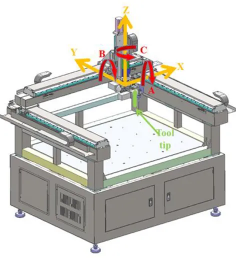
1.4 Proposed Measurement and Validation Procedure ... 8
Chapter 2 Scenario ... 9
2.1 Scenario Introduction... 9
2.2 Coordinate Measurement Machine in iCeiRA ... 10
2.2.1 Mechanism Design of Multi-axis CNC Robot ... 10
2.4.2 Data Extraction from CAD model ... 19
2.4.3 Geometrical Characteristics Computation ... 21
2.5 Simulation Workspace ... 24
Chapter 3 CMM Kinematics ... 26
3.1 Spatial Descriptions and Transformation ... 26
3.1.1 Three-Angle Representation ... 27
3.1.2 Angle–Axis Representation ... 28
3.1.3 Unit Quaternions ... 29
3.2 Differential Motion ... 32
3.3 CMM Kinematics ... 34
3.3.1 Forward Kinematics of CMM ... 34
3.3.2 Velocity Relationship: The Manipulator Jacobian ... 36
3.4 Forward Kinematics Model of iCeiRA CNC robot ... 38
3.5 Inverse Kinematics Model of iCeiRA CNC robot ... 40
3.5.1 Numerical Solution - The Jacobian Transpose Method ... 40
3.5.2 Analytic Solution – Closed-Form Solution ... 41
3.6 Linear Blending Motion ... 44
Chapter 4 Workpiece Registration ... 45
4.1 Description ... 45
4.2 Reference-based Registration ... 47
4.3 Algorithm-based Registration ... 51
Chapter 5 Freeform Surface Measurement and Validation ... 55
5.3.1 Joint Limit Consideration ... 58
5.3.2 Collision Detection ... 58
5.4 Measurement Trajectory Generation ... 62
5.4.1 Probing Posture Determination ... 62
5.4.2 Initial Trajectory generation ... 64
5.4.3 Joint Limit Response ... 67
5.4.4 Collision Response ... 69
5.5 Error Consideration ... 72
5.5.1 Pretraveling problem ... 73
5.5.2 Radius Compensation ... 74
5.6 Surface Validation ... 75
5.6.1 Localization Uncertainties ... 77
5.6.2 Reconstruction Uncertainty ... 79
5.6.3 Surface Validation ... 80
Chapter 6 Experiment ... 82
6.1 Localization Experiment ... 82
6.2 Freeform Surface Measurement Experiment ... 84
6.3 Data Analysis and Surface Validation ... 87
Chapter 7 Conclusion ... 90
REFERENCE ... 91
LIST OF FIGURES
Fig. 1-1 Common types of CMM ... 3
Fig. 1-2 Inner structure of a standard probe ... 4
Fig. 1-3 sensors or peripherals for CMM ... 5
Fig. 1-4 IGES file example ... 7
Fig. 1-5 STL object example ... 8
Fig. 1-6 proposed freeform surface measurement and validation process ... 8
Fig. 2-1 Scenario of measurement task ... 9
Fig. 2-2 Gantry-type machine and manipulator... 10
Fig. 2-3 The CAD diagram of the multi-axis machine tool with gantry-type and the its axis definition. ... 11
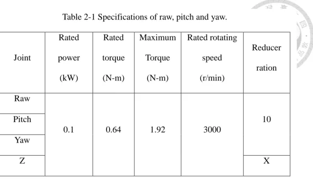
Fig. 2-4 Engineering drawing of AC servo motor ... 12
Fig. 2-5 The Engineering drawing of the reducer which is manufactured by APEX Inc.14 Fig. 2-6 slot-type photomicrosensor ... 15
Fig. 2-7 Integration of a high accuracy probe into CNC robot to reach the functionality of CMM ... 16
Fig. 2-8 measured workpiece... 17
Fig. 2-9 NURBS surface onto the workpiece ... 20
Fig. 2-10 NURBS surface in mesh-type ... 21
Fig. 2-11 Normal vector of the designed surface ... 22
Fig. 2-12 Principal direction of a point... 23
Fig. 3-1 the algorithm pseudo code of computing a quaternion convert from a
rotation matrix ... 31
Fig. 3-2 definition of standard D-H parameters ... 35
Fig. 3-3 the assigned DH link frames and ... 38
Fig. 3-4 The procedure of numerical method for solving IK ... 41
Fig. 3-5 The IK result working on an irregular path ... 43
Fig. 3-6 Linear blending motion... 44
Fig. 4-1 Workpiece Registration ... 46
Fig. 4-2 Effect of inaccurate localization ... 47
Fig. 4-3 Obtain normal vector of the surface... 48
Fig. 4-4 normal vectors of the referenced surface ... 49
Fig. 4-5 localize the translation of WCS by probing strategy ... 51
Fig. 4-6 schematic diagram of ICP algorithm ... 52
Fig. 4-7 Result of geometrically stable sampling for ICP algorithm ... 54
Fig. 5-1 Schematic diagram of the measured point generator ... 57
Fig. 5-2 Skeleton of the iCeiRA CNC robot 3D model ... 59
Fig. 5-3 Skeleton of the iCeiRA CNC robot ... 60
Fig. 5-4 example of collision detection where the collision happen on Link 2 ... 61
Fig. 5-5 Skeleton of the iCeiRA CNC robot ... 62
Fig. 5-6 Path with optimized posture determination ... 63
Fig. 5-12 Path modified by joint limit ... 68
Fig. 5-13 CMM motion on path with joint limit response ... 68
Fig. 5-14 Example of workspace to C-space for a 2D translating robot ... 70
Fig. 5-15 Simplified measured surface which is used for collision avoidance ... 70
Fig. 5-16 C-space example for a simple 2DoFs robot manipulator... 71
Fig. 5-17 Path modified with consideration of joint limit and collision ... 71
Fig. 5-18 CMM motion on path with joint limit and collision response ... 72
Fig. 5-19 Error in the measurement process ... 73
Fig. 5-20 schematic diagram of pretraveling problem ... 74
Fig. 5-21 schematic diagram of radius compensation ... 75
Fig. 5-22 schematic diagram Error caused by different reasons ... 76
Fig. 5-23 Freeform surface inspection considering the uncertainties in measurement, localization and surface reconstruction ... 76
Fig. 5-24 Reconstruction error and localization error ... 79
Fig. 6-1 Implementation of reference-based localization ... 83
Fig. 6-2 Implementation of freeform surface measurement ... 84
Fig. 6-3 The first reconstructed surface compared with CAD model ... 85
Fig. 6-4 Surface reconstruction result with different number of measured points ... 85
Fig. 6-5 The final reconstructed surface compared with CAD model ... 86
Fig. 6-6 Error descent of reconstruction error ... 86
Fig. 6-7 The resultant error distribution ... 87
Fig. 6-8 3D printer used to manufacture the workpiece ... 89
LIST OF TABLES
Table 2-1 Specifications of raw, pitch and yaw. ... 13
Table 3-1 link parameter of iCeiRA CNC robot ... 39
Table 5-1 Joint Limit of iCeiRA CNC robot ... 58
Table 6-1 Localization Result ... 83
Chapter 1 Introduction
This thesis main topic is a measurement process for complex surface inspection which works on a 7-DoF coordinate measurement machine with probing system. The principal and method will be figured out in the subsections below. Actually, the ideal of the main topic is gradually constructed by the experience of developing the robot control system and useful functions during my master career. The overview of this thesis and the simplified control scheme of the coordinate measurement system will be shown in this chapter.
First, the era of CMM is in section 1.1 and then section 1.2 introduces the task we would like to reach and some detail about the freeform surface measurement. Besides, the reason why we choose freeform surface as measured object is explained. Second, datatype and detail about the 3D CAD model are listed in section 1.3, including the most common one in industry, IGES, and the one for 3D printer, STL. Then the measurement procedure we purposed in this thesis is shown in section 1.4.
1.1 Era of Coordinate Measurement Machine
As the industry grows up rapidly in these years, accuracy of a workpiece is an important issue that more and more researches pay attention on. For a real workpiece fabricated from the computer numerical control (CNC) machines, there must exists error compared with the computer aided design (CAD) model. However, for some special industry such as aerospace industry, the accuracy of a workpiece is necessary to be promised. Therefore, coordinate measurement machines (CMMs) are utilized to validate the extent of difference between a real workpiece and its corresponding CAD model.
present coordinate instantly.The typical 3D "bridge" CMM is composed of three axes, X, Y and Z. These axes are orthogonal to each other in a typical three-dimensional coordinate system. Each axis has a scale system that indicates the location of that axis.
The machine reads the input from the touch probe, as directed by the operator or programmer. The machine then uses the X, Y, Z coordinates of each of these points to determine size and position with micrometer precision typically. By precisely recording the X, Y, and Z coordinates of the target, the accuracy of a workpiece can be measured and analyzed via regression algorithm for the construction of features.
In Fig. 1-1, three basic types of measurement machines are listed: (a) Bridge CMM is well known for its stability. And it provides cost-effective solution for dimensional quality control, (b) Gantry CMM is suited to inspection for large workpieces because synchronous gantry control leads to high speed movement. It can achieve larger workspace for measurement and efficient performance, (c) Horizontal Arm CMM is the most flexible type. The advantage is particular apparent when inspecting sheet metal parts in the car industry, or other large-volume components in the aerospace, ship, defense industries. Its open structure permits direct access to the workpiece and therefore significantly eases loading and unloading. (d) Shop floor conditions may suggest that accurate measurement results on the factory floor would be impossible to obtain. However, using specialized shop floor hardened CMM, measurement accuracy is ensured even in the production environment.
contact a point on the workpiece. On the other hand, Non-contact probes are best for parts that are either more complex, smaller, high-precision or easily deformable. They are either laser-based or vision-based.
(a) (b)
(b) (d) Fig. 1-1 Common types of CMM
(a) NIKON ALTO Bridge CMM (b) Perceptron COORD3 MCT Gantry CMM (c) Hexagon DEA MERCURY Horizontal Arm CMM (d) Hexagon TIGO shop floor
Take some useful sensors or peripherals for example: (a) ultra-compact probe features strain gauge technology. It delivers unrivalled submicron performance when applied to complex 3D shapes and contours, (b) probe head provides extra degree of freedom, which provides larger workspace and decrease time-cost furthermore. Besides, with adaptive control, the touch trigger probe is able to acquire data quickly by using
“sliding” touch onto a surface. (c) laser sensor uses a concentrated beam of light instead of a stylus. The beam acts as an optical switch so that when it is projected onto the part, the position can then be read by triangulation through a lens in the probe receptor. (d) For vision sensor, the 2D light sensitive CCD and the integral LED illumination allow
Fig. 1-2 Inner structure of a standard probe
1.2 Freeform Surface Inspection and Validation
It’s undeniable that the freeform surface inspection technique is thought to be one of the most valuable challenges in of measurement applications. Because of complex structure and irregular shape, it’s very hard to decide measured points by human intuitive. Therefore the geometrical characteristics of a surface should be analyzed to sample out to be a point set which can fully describe the whole surface. However, from
(a) (b)
(c) (d) Fig. 1-3 sensors or peripherals for CMM
(a) Renishaw OMP400 probe (b) Renishaw PH20 probe head (c) Nikon InSight L100 laser scanner. (d) Hexagon HP-C-VE vision sensor
has its own consideration. This thesis tries to solve the problem above and build a complete inspection system for complex surface inspection. The final target is to evaluate a real workpiece with complex surface, and validate the precision by comparing the measured data with CAD model.
1.3 CAD Model Representation
In this thesis, the CAD model of measured object is presented in IGES format. All geometrical data is extracted from the file and do some geometrical characteristics analysis. Besides, the mesh-type data format, STL format, is still used to describe other geometrical properties in the measurement process. Both the data type is briefly introduced below.
1.3.1 IGES File Specification
The Initial Graphics Exchange Specification (IGES) outlines a file format for the transfer of geometry data and CAD models. It can be used to represent both Boundary-Representation (B-Rep) and Constructive Solid Geometry (CSG) geometries, as well as two dimensional CAD diagrams. The file is an ASCII text based format, having each line be exactly 80 characters long. The file is split into five sections, denoted by the specific upper case letter in the 73rd column. Those sections are Start (S), Global (G), Data Entry (D), Parameter Data (P), and Terminate (T) sections. The Data Entry and Parameter Data sections are commonly abbreviated Data Entity (DE) and
1.3.2 IGES File Specification
An STL file is a triangular representation of a 3D surface geometry. The surface is tessellated logically into a set of oriented triangles (facets). Each facet is described by the unit outward normal and three points listed in counterclockwise order representing the vertices of the triangle. While the aspect ratio and orientation of individual facets is governed by the surface
(a)
Fig. 1-4 IGES file example
(a) IGES content (b) geometry presented by (a)
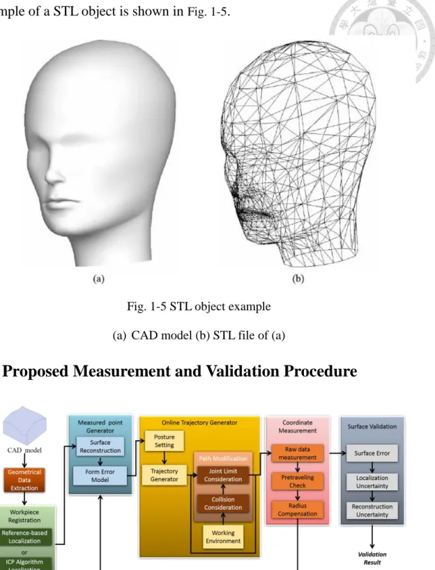
example of a STL object is shown in Fig. 1-5.
1.4 Proposed Measurement and Validation Procedure
Fig. 1-5 STL object example (a) CAD model (b) STL file of (a)
Chapter 2 Scenario
2.1 Scenario Introduction
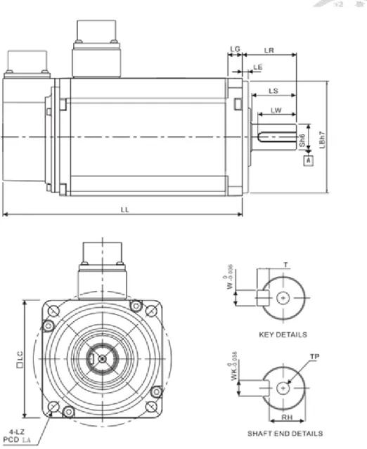
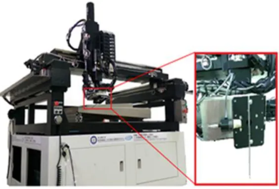
In this thesis, a measured workpiece with complex surface is placed onto the backside of CMM platform, where there still exist other objects on the platform. These objects are not measured target in this thesis so that we take them as obstacles in the workspace. The CMM we use in this thesis is a CNC robot with 7 axes and 6 degree of freedom (DoF). A touch trigger probe is mounted on the end-effector to probe the measured points and obtain coordinate data feedback. Each part mentioned above will be introduced in the following sections. The scenario is shown in Fig. 2-1.
2.2 Coordinate Measurement Machine in iCeiRA
We combine manipulator and gantry-type CNC machine tool to develop a new page in the machining field. Robot with gantry-type machine tool has many advantages like high stiffness, high accuracy and easy to calculate its coordinate system, for example, Fig. 2-2(a). Robot arm is connected by joints that allowing either translational (linear) or rotational motion as shown in Fig. 2-2(b). Combining the advantages of robot arm and gantry-type CNC machine tool has extra joints to apply and has more workspace than traditional type. The CNC robot is also designed and implemented in iCeiRA laboratory.
(a) (b) Fig. 2-2 Gantry-type machine and manipulator
(a) Gantry-type machine tool with linear motor. (b) Multi-axis robot arm.
at linear axis including X, Y and Z axis to control translation and three rotational axes which orthogonal to each other at the manipulator to control orientation. The x and y axes are using linear motor. The z axis and other three rotational axes are using AC servo motor which is manufactured by Delta Electronics as figure, Inc. The CAD diagram and specifications of AC servo motor and reduction ratio are shown in Fig. 2-4 and Fig. 2-5.
Fig. 2-3 The CAD diagram of the multi-axis machine tool with gantry-type and the its axis definition.
Fig. 2-4 Engineering drawing of AC servo motor
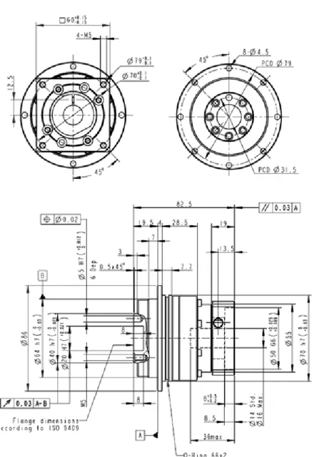
The diagram of reducer is shown in Fig. 2-5. The other characteristic is that most of crucial components like reducer, AC servo motor and screw are made in Taiwan. We want to convey a concept that we can build up a series outstanding machine tool industry by ourselves. We can obtain good effect by using planetary reduction gear and cost lower price than using harmonic drive.
Table 2-1 Specifications of raw, pitch and yaw.
Joint
Rated power (kW)
Rated torque (N-m)
Maximum Torque
(N-m)
Rated rotating speed (r/min)
Reducer ration
Raw
0.1 0.64 1.92 3000
10 Pitch
Yaw
Z X
Fig. 2-5 The Engineering drawing of the reducer which is manufactured by APEX Inc.
2.2.2 Anti-collision sensor and Home sensor
In order to avoid the motors collision or exceed the workspace, CNC robot is equipped with several sensors at every axis. Besides, home sensors are also mounted to define zero point for each axis. All sensors are the same slot-type photomicrosensor, which works as optical switches to control the signal output. The specification is shown in Fig. 2-6(a). For X and Y axes, two sensors are equipped at the end of linear motor for defining the boundary for each axis. Besides, a home sensor is mounted next to one boundary sensor to set the zero point. The remained axes, Z, A, B and C, have home sensors only. Fig. 2-6(b) shows the sensors located on Y axis.
(a) (b) Fig. 2-6 slot-type photomicrosensor
(a) Specification of sensor (b) location of sensors on Y axis
2.2.3 High accuracy probe
We integrate a high accuracy probe into CNC robot to be a second end-effector, so that a coordinate measuring machine (CMM) that we will mention behind the conclusion is born. The illustration is shown in Fig. 2-7. The probe has a precision ruby tip for reduced wear and increased accuracy. The shank is 3/8 inch diameter, to accommodate the capacities of the small desktop mills.
Fig. 2-7 Integration of a high accuracy probe into CNC robot to reach the functionality of CMM
2.3 Measured Workpiece
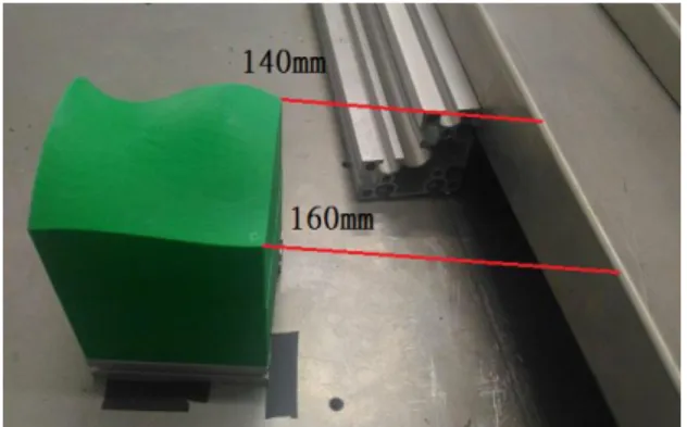
To build a complex surface to validate, we need to design a workpiece with some properties. First, any evident characteristics that can be identified by human intuitive is not appeared. Since an obvious feature can be easily utilized to infer measured points, which is not fitting to our purpose in this thesis. Second, the surface should be smooth enough, which means that every point onto the surface should be continuous. This condition is applied to fit the definition of “curvatured” surface. The condition is achieved by a continuous mathematic representation. Third, the surface should be bounded into a finite range. The largest range should not exceed the workspace of CMM.
On the basis of the restriction above, we utilized the famous CAD software, SolidWork, to design the measured workpiece. The complex surface onto the surface is randomly tuned as the Fig. 2-8(a) and the real object is fabricate by 3DP as shown in Fig. 2-8(b).
(a) (b) Fig. 2-8 measured workpiece
(a) CAD model of measured workpiece (b) real object
2.4 Geometrical Data Extraction
Before inspection process is implemented on the measured surface, we need to extract some geometrical data from CAD model, which is also the first step in the proposed measurement procedure. The data is used to be material for inspection process.
The extraction method mainly depends on the characteristics and mathematical model of the surface. For our workpiece, the surface is constructed by Non-uniform Rational B-Splines (NURBS) which is a mathematical model commonly used in computer graphics for generating curves or surfaces. The feature of this model is that it can be efficiently handled by computer programs and yet allow for easy human inter action.
Moreover, for a surface composed of several NURBS patches, the geometric continuity is promised perfectly with different levels including positional continuity (𝐺0), tangential continuity (𝐺1), curvature continuity (𝐺2).
2.4.1 NURBS Specification
A NURBS curve is defined by its order, a set of weighted control points, and a knot vector. NURBS curves and surfaces are generalizations of both B-splines and Bézier curves and surfaces, the primary difference being the weighting of the control points, which makes NURBS curves “rational". The Control points determine the shape of the
degree plus one. The values in the knot vector should be in nondecreasing order, so (0, 0, 1, 2, 3, 3) is valid while (0, 0, 2, 1, 3, 3) is not. The general form of a NURBS surface of degree (p,q) is shown.
, , , ,
0 0
, , ,
0 0
( ) ( ) ( , )
( ) ( )
m n
i p j q i j i j
i j
m n
i p j q i j
i j
N u N v w P
S u v
N u N v w
(2-1)where 𝑁𝑖,𝑝 and 𝑁𝑗,𝑞 are the B-Spline basis function, 𝑃𝑖,𝑗 are control points, and the weighted 𝑤𝑖,𝑗 of 𝑃𝑖,𝑗 is the last ordinate of the homogeneous point 𝑃𝑖,𝑗𝑤. For a B-Spline generalization, the basis function is
1 1
,0
( ) 1, 0,
i i i i
i
if t t t and t t N t
otherwise
(2-2)
1
, , 1 1, 1
1 1
( ) i ( ) i j ( )
i j i j i j
i j i i j i
t t
t t
N t N t N t
t t t t
(2-3)
where 𝑇 = {𝑡0, 𝑡1, … 𝑡𝑚} is the set of knot vector with 𝑡𝑖 ∈ [0,1], and define the control points 𝑃0, … , 𝑃𝑛. Define the degree as
1
p m n (2-4)
The “knot” 𝑡𝑝+1, … , 𝑡𝑚−𝑝−1 are called internal knots.
2.4.2 Data Extraction from CAD model
In our case, the workpiece is designed by famous CAD software, SolidWorks. In the beginning, we design a cube with 100𝑚𝑚 × 100𝑚𝑚 × 100𝑚𝑚 then the top face of the cube is deformed randomly by the built-in function in SolidWorks. The CAD model is exported in IGES format and we use the MATLAB to analyze and extract the
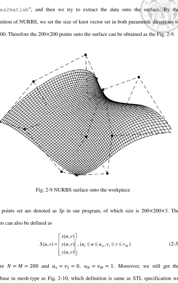
At first, the IGES file is imported in the MATLAB by the function
“iges2matlab”, and then we try to extract the data onto the surface. By the definition of NURBS, we set the size of knot vector set in both parametric directions to be 200. Therefore the 200×200 points onto the surface can be obtained as the Fig. 2-9.
The points set are denoted as Sp in our program, of which size is 200×200×3. The points can also be defined as
Fig. 2-9 NURBS surface onto the workpiece
programmability for computer graphic process.
2.4.3 Geometrical Characteristics Computation
To probe the measured points in normal direction and make some geometrical analysis, we need to infer some geometrical values about the characteristics of the surface, such as principal curvature, Gaussian curvature, mean curvature, principal angle, and normal vector. The following steps are the description about the mathematical inference about these values. All data is obtained from the mesh-type surface.
The normal vector is the vector perpendicular to the surface at the given point, Fig. 2-10 NURBS surface in mesh-type
a
N f b
c
(2-6)
where 𝛻𝑓 denotes the gradient. For the surface with parameterization 𝑥(𝑢, 𝑣), the normal vector is given by cross product of the partial derivatives.
x x
N u v
(2-7)
The result is shown as Fig. 2-11, all normal vector has two opposite directions. Here we choose the outward-pointing normal vector for displaying, while the inward-pointing normal vector is used as probing direction for implementing inspection.
derives their principal directions respectively. Physically it means how the surface bends by different amounts of different directions at the point.
The principal comes from the eigenvalues of the matrix, Ⅰ−𝟏Ⅱ, where Ⅰis first fundamental form and Ⅱ is second fundamental form.
u u u v
v u v v
X X X X
X X X X
(2-7)
uu uv
vu vv
X N X N
X N X N
(2-8)
where the subscript u,v means partial derivative and N is unit normal vector of the point.
Fig. 2-12 show the principal directions 𝑈⃑⃑⃑⃑⃑⃑⃑⃑⃑⃑ which represents the maximum curvature 𝑚𝑎𝑥 𝜅1 and 𝑈⃑⃑⃑⃑⃑⃑⃑⃑⃑ which represents the maximum curvature 𝜅𝑚𝑖𝑛 2.
Fig. 2-12 Principal direction of a point
only on distances that are measured in the surface. The sign of the Gaussian curvature can identify the characteristics of the surface. The result is shown in Fig. 2-13, where the values are displayed in color form.
2
1 2 2
1 2
1( )
2
eg f
K EG F
H
(2-9)
where E,F,G are first fundamental coefficients and e,f,g are coefficients of the second fundamental form.
2.5 Simulation Workspace
Fig. 2-13 Gaussian curvature for the surface
visualized to let the user certainly know what motions or postures cause dangers. We try to build a complete simulation workspace with physical parameters in reality. To save computation time and cost, the simulation range is limited into the space around the measured workpiece, which all postures of the CNC robot will be inside in. The simulation is shown in Fig. 2-14.
(a) Real working environment and physical parameter
(b) Simulation workspace
Fig. 2-14 Simulation workspace of real environment
Chapter 3 CMM Kinematics
In this chapter, mathematic of 3D spatial descriptions and basic kinematics are described. The kinematics of the iCeiRA CNC robot is also introduced in the late part of the section.
3.1 Spatial Descriptions and Transformation
We will use AV or Av to describe a point or a vector in this thesis, so we will not always use → to represent a vector. The upper-title means the vector is in terms of coordinates frame {A}. The subtitle can represent a specific point of a position;
represent a vector from point A to point B like PAB; or it can describe a position or a vector as a specific point or other specific meaning.
We can represent the orientation of a coordinate frame {B} by its unit vectors expressed in terms of the reference coordinate frame {A}. Each unit vector has three elements and they form the columns of a 3×3 orthonormal matrix ARB . The matrix is also a rotation transformation matrix that can transform points from frame {B} to reference frame {A}.
A 4×4 homogeneous transformation matrix has the structure like
,
0 0 0 1
A A
A B B o
B
R P
T
(3-1)
where “A” and “B” represent coordinate frames; “B,o” means it is an original point of
,
1 0 0 0 1 1
A A A B
B B o
P R P P
(3-2)
It is seen that implements the equation
,
1 1
A A B A
B B o
P R P P
(3-3)
It is obviously mapping the point P from frame {B} to {A}. Also, the inverse of the transformation matrix represents the inverse operation of this mapping, which is
BTA = (ATB)-1, BTAATB = I. The inverse of ATB can be derived as
1 ,
0 0 0 1
A T A T A
A B B B B o
B A
R R P
T T
(3-4)
3.1.1 Three-Angle Representation
Any 3×3 rotation matrix can be specified by just three parameters. A well-known method is ZYX Euler Angle representation:
( ) ( ) ( )
X Y Z
RR R R (3-5)
The inverse formula is:
if
11 12 13
21 22 23
31 32 33
r r r
R r r r
r r r
, then
2 2
31 11 21
32 33
21 11
atan2( , )
atan2( , )
atan2( , )
r r r
r c r c
r c r c
(3-6)
A fundamental problem with the three-angle representation is singularity. This
3.1.2 Angle–Axis Representation
Another method to describe Rotation is equivalent angle–axis representation: two coordinate frames of arbitrary orientation are related by a single rotation about some axis in space. Converting from angle and vector to a rotation matrix is achieved using Rodrigues’ rotation formula
3 3 sin S( ) (1 cos )( 3 3)
A A A A T
RBI u u u I (3-7)
noting that, the outer product Au uA T [S(Au)]2I3 3 . So another equivalent expression is
sin S( ) cos S( ) 2
A A A A A T
RB u u u u (3-8)
The meaning of this equation is rotating {B} relative {A} about the unit vector u by an angle θ according to the right-hand rule. Where S(u) is a 3×3 skew-symmetric matrix of the 3×1 vector u. A matrix S is defined as a skew-symmetric matrix if and only if ST S 0. It has zero diagonal and the property that v S vT ( ) 0, v. For the 3×3 case:
0
( ) 0
0
z y
z x
y x
v v
S v v v
v v
(3-9)
Finally, it can be shown that the rotation matrix is
11 12 13
21 22 23
31 32 33
( , )
A B
r r r
R u r r r
r r r
(3-11)
then
11 22 33 1
acos( )
2
r r r
(3-12)
and
32 23
13 31
21 12
1 2sin
A
r r
u r r
r r
(3-13)
The θ has a value between 0 and 180 degrees. For any solution (Au, ) , there is another pair solution (Au,),which results in the same orientation in space. Also, another problems of this method is that, when θ near to 0 or 180 degrees, the axis becomes ill-defined
3.1.3 Unit Quaternions
Quaternions have been controversial since they were discovered by W.R. Hamilton over 150 years ago but they have great utility in robotics, computer vision, computer graphic and aerospace navigation applications. The quaternion is an extension of the complex number – a hyper-complex number – and is written as a scalar plus a vector
w
w x y z
Q
i j k
(3-14)
where
w
, 3 and the orthogonal complex numbers, i, j and k are defined such that, ,
Q w x y z (3-16)
To represent rotations we use unit-quaternions. These are quaternions of unit magnitude, that is, Q 1 or w2 x2 y2 z2 1. The unit-quaternion has the special property that it can be considered as a rotation of θ about the unit vector
ˆn
which are related to the quaternion components byˆ cos , sin
2 2
w n
(3-17)
and is similar to the angle-axis representation of section 2.1.2. The transformation operation of rotation matrix is left-multiplication of matrix. The same operation in quaternion is known as Hamilton product, we denote it as Q2Q1 and
2 1 2 1 2 1 2 1 1 2 2 1
Q Q w w w w (3-18) It can be expressed as a matrix-vector product where
2 2 2 2 1
2 2 2 2 1
2 1
2 2 2 2 1
2 2 2 2 1
w x y z w
x w z y x
Q Q
y z w x y
z y x w z
(3-19)
As we can see, computing the Hamilton product requires 16 multiplications and 12 additions. But computing two orthonormal rotation matrices requires 27 multiplications and 18 additions. Quaternion is more efficiency.
According to Eq. (2-17), the quaternion can be algebraically manipulated into an
this basic form:
11 22 33
32 23
13 31
21 12
1 2
( ) /
( ) /
( ) /
w r r r
x r r w
y r r w
z r r w
(3-21)
but it tend to be unstable and un-accuracy when trace(R)+1 of the rotation matrix is zero or very small. a better algorithm to compute the quaternion from a rotation matrix is shown in Fig. 3-1.
Algorithm of computing
a Quaternion converted from a Rotation Matrix
tr(0) = R(0,0)+R(1,1)+R(2,2)+1;
tr(1) = R(0,0)-R(1,1)-R(2,2)+1;
tr(2) = -R(0,0)+R(1,1)-R(2,2)+1;
tr(3) = -R(0,0)-R(1,1)+R(2,2)+1;
for i=0:3 {
if( tr(i) < 0 ) tr(i) = 0;
s(i)= 0.5*sqrt(tr(i));
}
if(s(0)>=s(1) && s(0)>=s(2) && s(0)>=s(3)){
w = s(0);
x = sign(R(2,1)-R(1,2))*s(1);
y = sign(R(0,2)-R(2,0))*s(2);
z = sign(R(1,0)-R(0,1))*s(3);
}else if(s(1)>=s(0) && s(1)>=s(2) && s(1)>=s(3)){
w = sign(R(2,1)-R(1,2))*s(0);
x = s(1);
y = sign(R(1,0)+R(0,1))*s(2);
z = sign(R(0,2)+R(2,0))*s(3);
}else if(s(2)>=s(0) && s(2)>=s(1) && s(2)>=s(3)){
w = sign(R(0,2)-R(2,0))*s(0);
x = sign(R(1,0)+R(0,1))*s(1);
y = s(2);
z = sign(R(2,1)+R(1,2))*s(3);
}else if(s(3)>=s(0) && s(3)>=s(1) && s(3)>=s(2)){
w = sign(R(1,0)-R(0,1))*s(0);
x = sign(R(0,2)+R(2,0))*s(1);
y = sign(R(2,1)+R(1,2))*s(2);
z = s(3);
}
Fig. 3-1 the algorithm pseudo code of computing a quaternion convert from a rotation matrix
normalize the result. The normalization is achieved by ensuring that the quaternion norm is unity, a straightforward division all elements by the quaternion norm
Q Q
Q (3-22)
It is easier to normalize a quaternion rather than a non-orthogonal matrix. To summary, the advantages of using quaternion to represent rotation are list:
1. Quaternions doesn’t have gimbal lock problem but Euler angle representation does.
2. Quaternions composed from four numbers but rotation matrix need nine numbers.
3. Similar to rotation matrix, the product of two quaternions can represent twice rotations but the computation is less.
4. Easier interpolation between quaternions.
5. Quaternion, matrix operations will accumulate rounding error or integration error, so we need to do each of its normalization and orthogonalization. But "Restoring"
a rotation matrix is computationally more expensive than normalizing a quaternion.
3.2 Differential Motion
A body rotating in 3D space has an angular velocity which is a vector quantity ω = [ωx ωy ωz ]T. The direction of this vector defines the instantaneous axis of rotation, that is, the axis about which the coordinate frame is rotating at a particular instant of time. In general, this axis changes with time. The magnitude of the vector is the rate of rotation
0
( ) 0
0
z y
z x
y x
S
(3-24)
Consider the approximation of derivative
3 3
( ) ( )
( ) ( ) ( ) ( ( ) ) ( )
R t t R t R t
S R t t R t S t I R t
(3-25)
which describes how the orthonormal rotation matrix changes as a function of angular velocity.
Consider a coordinate frame that undergoes a small rotation from R0 to R1. Let the small rotation Δθ = ωΔt, Δθ = [Δθx Δθy Δθz ]T, ω = [ωx ωy ωz ]T. We can write (3-25) as
1 ( ( ) 3 3) 0 ( ( ) 3 3) 0
R S t I R S I R (3-26)
and rearrange it as
1 0 3 3
( ) T
S R R I (3-27)
and then apply the inverse operation of S(∙), defined as vex(∙), to both sides
1 0 3 3
vex(R RT I )
(3-28)
The detail of vex operator in 3×3 case is
32 23
3 1 3 3 13 31
21 12
v vex( ) 1 2
s s
S s s
s s
(3-29)
The Δθ = ωΔt is a vector that represents a small rotation about the world x-, y- and z- axes.
If we give two homogeneous transformation matrices T0, T1 to represent two poses (position and orientation) that has small deference, then we can represent the deference
1 0 6 1 0 1
1 0 3 3
( , ) ,
vex( T )
P P
T T R R I
(3-30)
Where T0 = (R0,P0), T1 = (R1,P1), In practice, this equation can be used to compute the deferential of motion in 3D space. Let T0 = T(t), T1 = T(t+Δt) and T= (R,P), than
dP t
dR t t
(3-31)
where υ and ω is instantaneous linear velocity and angular velocity at pose T and time t.
The character “d” will mean “small deference” or deferential conveniently in this thesis.
The inverse of Eq. (2-30) is
1
1 0 4 4 0
1 3
( )
( , ) ,
0 0
S dR dP dP
T T I T
dR
(3-32)
In practice, this equation can be used to compute the integration of motion in 3D space.
The example is trajectory generation. It will introduce in chapter 4.
3.3 CMM Kinematics
3.3.1 Forward Kinematics of CMM
A serial-link manipulator comprises a set of links in a chain and connected by joints. Each joint has one degree of freedom. Motion of the revolute joint changes the relative angle of its neighboring links while the prismatic one changes relative
a D-H representation is the following procedure:
First, the coordinate frames are assigned to the links by the following rules:
1. zˆj1 jthjoint axis
2. xˆj zˆj1 and point away from it 3. yˆj zˆj xˆj
4. {0}: zˆ01 jointst , {N}: xˆN zˆN1 , zˆN align with zˆN1
Then, we can determine the D-H parameter according to these frames by the following rules:
j: the angle from xˆj1 to ˆx measured about j zˆj1
d : the distance from j xˆj1 to ˆx measured along j zˆj1
a : the shortest distance from j zˆj1 to ˆz measured along ˆj x j
j: the offset angle from zˆj1 to ˆz measured about ˆj x j Fig. 3-2 definition of standard D-H parameters
1
, ,
( , , , ) ( ) ( ) ( ) ( )
i
i i i i i R z i z i x i R x i
T d a T T d T a T
(3-33)
which can be expanded as
1
cos cos sin sin sin cos
sin cos cos sin cos sin
0 sin cos
0 0 0 1
i i i i i i i
i i i i i i i
i i
i i i
a T a
d
(3-34)
For a revolute joint θi is the joint variable and di is constant, while for prismatic joint di
is variable and θi is constant and αi = 0.
The forward kinematics (FK) is often expressed in functional form with the end-effector pose as a function of joint coordinates (the coordinate frame of the end-effector is usually same as the last Nth coordinate frame). Using the product of the individual link transformation matrices for an N-axis manipulator is
0 0 1 1 1
1( )1 2( )2 i ( ) N ( )
E i i N N
T T q T q T q T q (3-35)
where “q” represents the joint space variable q = [q1 q2 …qi… qN]T . The 0TE include a rotation matrix and a position vector just describes the pose of the end-effector.
3.3.2 Velocity Relationship: The Manipulator Jacobian
If we write the FK in functional form as ( )
x f q (3-36)
and taking the derivative we write
Jacobian matrices are useful in robot arm inverse kinematics, trajectory planning and control. We can compute Jacobian matrices numerically by using Eq. (3-32) to approximate the derivative of transformation matrix with respect to joint coordinates.
We perturb ith joint by a small but finite amount dqi, and let T1 in Eq.(3-32) as T(qi+dqi) and T0 = T(qi), then, the vector Ji 6 1 which is ith column of the Jacobian matrix can be approximate as
( ), (i i i)
i
i
T q T q dq
J dq
(3-38)
In practice, we will prefer to compute Jacobian matrices in analytic form for efficiency in programing. In fact, we can get the symbolic form forward kinematic 0TE
and symbolic form of a Jacobian matrix by symbolic computation ability of the powerful software MATLAB. The derivation of a Jacobian matrix has two parts. First part is J 3 N , the translational part of the Jacobian matrix. Obviously, each column of Jv is partial differential of translational FK function with respect to each joint variable.
After we compute the FK 0TE = (0RE, 0PE) in terms of symbolic joint coordinate
1
q N , we can get the analytical Jv(q) which is
0 0 0 0
1 2
( ) [ E E E E]
i N
P P P P
J q q q q q
(3-39)
by input jacobian(0PE,q)in MATLAB. The jacobian() is a build-in function in MATLAB. Second part is J 3 N , the rotational part of the Jacobian matrix. The angular velocity of the end-effector is the sum of angular velocity of each rotation joints, we can write as 0E 0102 0N (0i 03 1 as it is prismatic joint). Because
velocity relation in matrix form, which is
0 1 1 1
1 2
1 for rotaional joint
ˆ ˆ ˆ ˆ
( ) ,
0 for prismatic joint
i N
i N i
J q z z z z (3-40)
Then, we can write Eq. (2-37) as
J q J
(3-41)
3.4 Forward Kinematics Model of iCeiRA CNC robot
iCeiRA CNC robot is a gantry-typed 6 axis machine. The high degree of freedom enables measurement task can be achieved with appropriate probe and control strategy.
Compared with common CMMs, the extra degree of freedom leads to more flexible machine posture for a probing point. Fig. 3-3 shows the assigned DH link frames and parameters of the CNC robot.
The detail geometry parameter and numerical value are list in chapter 5. Table 3-1 is the DH table according to the DH frames in Fig. 3-1. The first three joints are prismatic joints and the other three joints are rotational joint. Also, the joint limits are listed.
The joint 1, 2, 3 are prismatic joint which control the translation of gantry. The joint 4, 5, 6 are rotational joint, and their axes intersect at a single point at the center of joint 5. We can view this kind of structure as a single point at the intersection. In geometry, this kind of mechanism is called “vertical spherical joint” which have three DoF provide roll-pitch-yaw rotation work on the point of intersection. In industrial design field, this geometrical structure is called spherical joint architecture. The feature of this design is useful and convenient for computation of inverse kinematics which we will discuss in the next section.
Table 3-1 link parameter of iCeiRA CNC robot
i θi(rad) di αi ai U L
1 - Lx 90° 0 1000mm 0 mm
2 - 0 0° Ly 1000mm 0mm
3 - -Lz -90° 0 60mm 45mm
4 θ4 + 0 0 90° 0 170° 175°
5 θ5 + 0 0 90° 0 90° -10°
6 θ6 + 0 d
tool180° a
tool0° -135°
U: joint angle upper bound L: joint angle lower bound