Using Spectral and Spatial Information for Oil Spill Detection in Multi-spectral Imagery

Volume 13, No.4, December 2008, pp. 285-294

1 PhD Candidate, Institute of Applied Geosciences, National Taiwan Ocean University Received Date: Jan. 01, 2008

2 Professor, Institute of Applied Geosciences, National Taiwan Ocean University Revised Date: Feb. 17, 2008

3 MS Student, Graduate Institute of Space Science, National Central University Accepted Date:Mar. 09, 2009

4 Associate Professor, Center for Space and Remote Sensing Research, National Central University

Using Spectral and Spatial Information for Oil Spill Detection in Multi-spectral Imagery

Hung-Ming Kao ¹ Ling-Ling Tsao ² Chao-Shing Lee ³ Hsuan Ren ⁴

ABSTRACT

Oil spill on the sea surface produced by human activities is disastrous to the ecological environment. How to detect, monitor and track the oil spill are always very important tasks. Due to oil spill often occur in open sea, remotely sensed image provides an effective technology to monitor the sea area. But the oil spill only occur in a very small are in the image, therefore, to detect the oil spill on the sea surface is a challenge problem. This study focuses on the detection of oil slick on sea surface using both spectral and spatial information of the remotely sensed images. Since the oil spill area usually only occupies a few pixels in the image scene, it can be considered as anomaly. By applying anomaly detection algorithm with only spectral information, the oil spill area can be extracted along with other marine phenomena as interference. In order to eliminate the interferences, spatial features are introduced. The experimental result shows the proposed method combining the spatial features of oil spill with spectral information improves the oil spill detection performance.

Keywords: oil spill, anomaly detection, RX detector (RXD), spatial feature.

1. Introduction 

Taiwan plays an important role in marine transportation in southeastern Asia. Nowadays, marine transit is still an important way for import and export. The oil spill on the sea surface caused by human activities occurs from time to time and is harmful to the marine environment. Using the remotely sensed images to detect this unwelcomed hazard material on the sea surface is a convenient and effective approach.

Based on the carrier types, the remote sensing sensors are categorized into airborne and space-borne. The former are mounted on the airplanes and can provide images with higher spatial resolution. But the cost for each data collection mission is usually high. On the other hand, the latter ones are mounted on the satellites. Besides its relatively low price, it can provide images with larger field of view and fair resolution which is suitable for oil slick detection. Categorized by the frequency bands of the electromagnetic wave, the active laser fluorosensor performs the best for detecting the oil slick, and then the active radar wave. For the passive sensors, the infrared and ultraviolet also perform well, while the visible region is easily interfered by other materials. Therefore, it is not

suggested to use only the visible bands (Fingas and Brown et al., 2000).

The active radar remote sensing is widely used for oil slick detection (Del Frate et al., 2000;

Lopez et al., 2005; Taylor, 1992), because the oil will reduce the reflection energy of radar and yield the dark area in the image. But because of its speckle noise, high price and long revisit period, it is usually difficult to process the data and may not able to collect images on the events.

Our purpose is to develop a high performance algorithm to detect oil slick with the easily acquired optical satellite images.

Target detection can be implemented in two aspects. One is using target’s unique characteristics of spectral reflection; the other is using the spatial textural distribution to discriminate them from the background. Since the spectral information between oil slick and the surrounding sea water were very different, and it usually only occupied a few pixels, the famous RX algorithm (Kelly, 1989; Reed and Yu, 1990) is adopted to detect the oil slick as an anomaly. Although it can detects oil slick area, but the result also extracts other interferers produced by marine phenomenon. In order to reduce the influence of the interference, we introduce the Spatial Feature Information (Liao, 2001; Huang, 2006) and adopt the spatial

textures to discriminate oil slick from the background. After applying Spatial Feature Information algorithm, the differences between oil slick and background can be easily revealed.

Therefore, the RX algorithm is implemented on both spectral and spatial features and the oil slick area can get higher separation from the background. Finally, a thresholding operation is applied to locate the oil slick area.

2. Anomaly Detection 

Target detection is to extract target of interests from the background materials, while anomaly detection is to detect targets with the following two properties. Firstly, they are small targets and occupy only a few pixels in the image scene, and secondly, they have distinct spectrum from the background. The oil spill on the sea surface satisfies these two properties.

Therefore, in our study, we view oil slick as an anomaly, and adopt the RX algorithm for anomaly detection.

2.1. RX Algorithm 

The RX algorithm was development by Reed and Yu (1990) based on generalized likelihood ratio test (GLRT) with Gaussian distribution for likelihood function. It can detect anomalies without any priori information of target or background (Kelly, 1989).

) ( )

( μ ¹ μ

δ_RX = r− ^TK_L⁻_×L r− (1) where r is the vector of pixel, L is the number of spectral bands, μ is the global sample

mean vector and

∑

=

× = ^N − −

i

T i i L

L r r

K N

1

) )(

1 ( μ μ is the sample covariance matrix of the image.

Since some pixels have very different spectrum from others, they give higher score with Eq. (1) on image, and then the anomaly pixels can be found.

We decompose the sample covariance matrix with eigenvector analysis (Chen, 2006), then the covariance matrix can be rewritten as Eq. (2).

Λ

× A= K

A^T _LL (2) where A and Λ are the eigenvector and eigenvalue matrixes of KL ^× L respectively.

Substitute Eq. (2) into (1), the RX can be viewed as,

)]

( [ )]

( [

) ( )

(

) ( )

(

) ( ) (

2 / 1 2 / 1 1 1

μ μ

μ μ

μ μ

μ μ

δ

−

×

−

×

=

− Λ

Λ

−

=

− Λ

−

=

−

−

=

−

−

−

−

×

r s r s

r A A

r

r A A r

r K r

T

T T

T T

L L T RX

(3)

where

s = Λ

A

From Eq. (3), we know RX algorithm is equivalent to removing the correlation between bands with whitening process and then calculate the Euclidean distance to the origin. If there is a pixel with distinct spectrum from the background, its distance to the origin will be large, and it will be detected by RX algorithm as an anomaly.

3. Spatial Feature Information 

Spatial Feature Information calculates the relationship between the gray level value of one pixel and its surrounding pixels in the image.

Spatial features could catch the texture, boundary and shape information. In this study, we adopt two kinds of Spatial Feature Information (Huang, 2006): Gray Level Histogram and Texture Feature Coding Method.

3.1. Gray Level Histogram

Gray Level Histogram (Christoyianni et al., 2000) was extracted from the distribution of pixel brightness in the image. It can be calculated by the probability of each gray level (p(k)) in the image with their gray value (k) according to the statistic property. For example, in an 8-bit image, the gray level is from 0 to 255.

Mean:

∑

=

⋅

=²⁵⁵

0

) (

k

k p

μ k (4) Variance:

∑

=

⋅

−

= ²⁵⁵

0 2

2 ( ) ( )

k

k p k μ

σ (5)

Kurtosis:

∑

=

−

⋅

−

= ²⁵⁵

0 4

4 4 ( ) ( ) 3

4 1

k

k p k μ

μ σ (6)

3.2. Texture Feature Coding Method

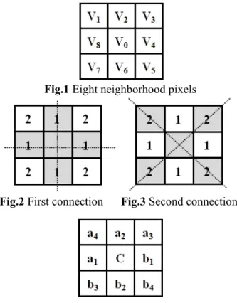
Texture Feature Coding Method computes the relation of central pixel’s four directions variation in the eight neighborhood pixels (Fig.

1). The four directions are first connection:

horizontal direction (0˚-180˚) and vertical direction (90˚-270˚) which shows in Fig. 2;

Second connection: the upper right to lower left (45˚-225˚) and the upper left to lower right (135˚-315˚) which shows in Fig. 3. In order to code pixels in image, it takes a 3×3 mask on

Information for Oil Spill Detection in Multi‐spectral Imagery pixel in image and gives those nine pixels a

serial number which shows in Fig. 4.

Fig.1 Eight neighborhood pixels

Fig.2 First connection Fig.3 Second connection

Fig.4Texture feature code

Where C is the central pixel and its surrounding eight pixels are marked as {a1, a2, a3, a4, b1, b2, b3, b4}. Selected three pixels on four directions variously and calculated odds of two neighbor pixels. According to the variation of three pixels on same direction we could code pixels in image. There are four possible situations with three connected pixels in one direction (Δ is the tolerance error):

I. (|a_i-C| Δ)∩(|C≦ -b_i| Δ)≦

If the differences between the connection pixels are within the tolerance error, it is viewed as unchanged.

II. [(|a_i-C| Δ)∩(|C≦ -b_i|>Δ)] [(|a∪ _i-C|>Δ)∩(|C-b

i| Δ)]≦

The difference of one connection pair is within the tolerance error, and another exceeds that value.

III. [(ai-C>Δ)∩(C-bi>Δ)] [(C∪ -ai>Δ)∩(bi-C>Δ)]

The three connection pixels are increase or decrease monotonically and the differences exceed the tolerant error.

IV. [(a_i-C>Δ)∩(b_i-C>Δ)] [(C∪ -a_i>Δ)∩(C-b_i>Δ)]

The middle pixel has maximum or minimum value and both connection pairs have differences exceed the tolerant error.

Where the Δ is the tolerance error, and there are two ways to assign this parameter: one is fixed relation with Δ between 1 and 3; another way is Just Noticeable Difference (JND).

⎪⎩

⎪⎨

⎧

<

+

−

≥ +

= −

127 ,

3 ) 127 (

127 ,

3 ] 127)}

( 1

[ ¹²

bg if bg

bg bg if

JND β

α (7)

According to table 1, the classified number is given by combining the direction of the first and second connection.

Table 1Texture feature coding method classification

1st connection

2nd connection

Category I II III IV I 1 2 3 4 II 2 5 6 7 III 3 6 8 9 IV 4 7 9 10

Define κ as the classified result of combining horizontal direction and the upper right to lower left direction, λ as the classified result of combining vertical direction and the upper left and lower right direction. The texture feature number (TFN) is the multiplication of κ and λ for each pixel, as shown in Eq. (8).

) , ( ) , ( ) ,

(x y x y x y

TFN =α ×β (8) TFN has 42 possible numbers between 1 and 100, and it is rearranged into 0 to 41. If the number is large, then the pixel’s gray value is difference from its neighbor, on the other hand, if the pixel has similar gray value to its surroundings, the number will be small. There

are three indexes calculated from TFN as following:

3.2.1. Coarseness

Coarseness counts the frequency of the largest TFN. For the largest number of TFN, the pixel is classified as situation IV in all four directions, i.e. TFN is 41.

∑

=

Δ Δ

=

*

0

) 41 ( P

Coarseness (9)

} 41 ,..., 2 , 1 , 0 { ) , (

)), , ( )) (

, ( (

∈

= ^Δ

Δ

y x TFN

N y x TFN y N

x TFN

P (10)

Where PΔ is histogram of TFN, NΔ is TFN occurring times and N is the number of occurring times for all TFN.

3.2.2. Homogeneity 

Similar to the concept of coarseness, Homogeneity counted the smallest variation’s occurring frequency in TFN. The number of TFN is zero.

∑

=

Δ Δ

=

*

0

) 0 ( P y

Homogeneit (11) 3.2.3. Mean Convergence   

Mean Convergence can evaluate the closeness between TFN and average.

∑

Δ −

= ⁴¹

0 *

*

*( ) |

|

n

n p MC n

σ μ

‧ (12)

Where ^μΔ* is TFN’s average when tolerance error equal to Δ^* , σΔ^* is TFN’s standard deviation when tolerance error equal toΔ^*_.

3.2.4. Variance 

Variance indicates the variation between number of TFN and its mean. If the variation is larger variance would be greater.

) ( )

( * *

41 0

2 P n

n Variance

n Δ

= Δ

∑

= μ (13)

4. Experimental Result 

The experiments contain two parts, a computer simulation and a real remote sensing image scene. We adopt SPOT-1 multispectral images for the experiments, and the synthetic scene for simulation is generated with the oil

and sea water spectrum extracted from this image. The SPOT-1 has three bands, green (0.5 mm-0.59 mm, band1), red (0.61 mm-0.68 mm, band2) and near IR (0.79 mm-0.89 mm, band3) with 12.5 meters spatial resolution. On Jan. 14, 2001, the Amorgos was grounded on the sea shore of Long-Luan Pool, Kenting. (Liu, 2007).

Under the gale and wave, the cargo ship was broken and the oil is spilled on the sea. As shown in Fig. 5, SPOT-1 captured the whole scene of coast of Kenting on Jan. 17. The oil slick is distributed from northeast to southwest.

(a) (b) (c)

Fig.5Original SPOT-1 images

4.1. Computer Simulation

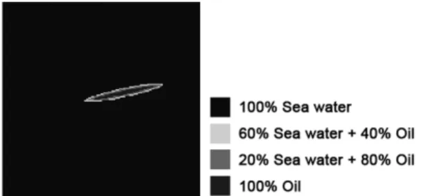
The spectrum of the oil spill and pure sea water (Fig. 6) are extracted manually from the image scene for synthetic image scene generation. Two cases are simulated with different oil slick distributions, and the detection performances are analyzed.

Fig.6 Spectrum of oil slick and sea water In case 1, the oil slick is a circular distribution. The abundance map is shown in Figure 7, where the spectrum of mixed pixels is linear combined of the spectrum of sea water and oil with assigned abundance fractions. The simulated oil slick pixels contain 96, 112 and 108 pixels with 100%, 80% and 40% of oil slick respectively. The Gaussian noise is added to each pixel with signal-to-noise ratio (SNR) equals to 30.

Information for Oil Spill Detection in Multi‐spectral Imagery

Fig.7Abundance map for case 1

Fig.8Four detection scenarios

(a) Scenario 1 (b) Scenario 2

(c) Scenario 3 (d) Scenario 4 Fig.9Threshold results for Case 1 There are four different scenarios for the oil slick detection (Fig. 8): (1) only use the spectral information, i.e., the original SPOT-1 images; (2) purely use the spatial feature information

extracted from the original images; (3) combine spectral information and spatial feature information extracted from result in (1); (4) combine both spectral and spatial feature information, i.e., the images from the (1) and (2) scenarios.

The threshold results of four scenarios are shown in Figure 9. It clearly shows that scenario 4 has the fewest interference pixels. The detection probability and error rate are calculated before and after the morphologic operations for performance analysis in table 2. It is worth noting that the morphologic operation can significantly reduce the error while also increase the detection rate. Among four scenarios, the detection with spectral information and spatial features extracted from original bands yields the best result, while the use of only the spectral information gives the worst one.

Table 2Performance analysis for simulation case 1 Scenario Correct Detection Error

pixels % pixels % 1 Before 254 80.38 491 1.22

After 257 81.33 59 0.15 2 Before 265 83.86 351 0.91

After 264 83.54 52 0.14 3 Before 283 89.56 320 0.83

After 304 96.20 18 0.05 4 Before 306 96.84 283 0.73

After 316 100.00 1 0.00 Oil slick: 40%:108 pixels 80%:112 pixels;100%:96 pixels

For case 2, we simulate the oil slick is starched by wind and ocean waves to an oval distribution. The abundance map is shown in Figure 10 with generation process the same as case 1. The simulated oil slick pixels contain 207, 204 and 157 pixels with 100%, 80% and 40% of oil slick respectively. The threshold results of four scenarios are shown in Figure 11.

It also shows that scenario 4 has the fewest interference pixels. In table 3, it is noticed that the morphologic operation can reduce the error but also reduce the detection rate. This is because this operation considered the two ends of the oil slick as small detected areas and removed them with interference. Among four scenarios, the detection with spectral information and spatial features extracted from original bands still yields the best result, while the use of only the spatial features performs the worst.

0 0 0 0 0 0 0 0 0

Fig.10 Abundance map for case 2

(a) Scenario 1 (b) Scenario 2

(c) Scenario 3 (d) Scenario 4 Fig.11 Threshold results for Case 2

Table 3Performance analysis for simulation case 2 Case Correct Detection Error

pixels % pixels % 1 Before 411 72.36 347 0.87

After 342 60.21 226 0.57 2 Before 372 65.49 446 1.16 After 318 55.99 250 0.65 3 Before 429 75.53 294 0.77 After 353 62.15 215 0.56 4 Before 420 73.94 294 0.77 After 408 71.83 160 0.42

4.2. Real Image Scene 

For the real image scene, we first remove the land area as a preprocess step. Based on the strong absorption of the water in IR region, we separate the land area from the sea by a threshold. Figure 12 shows the original images with land area removed.

For the first scenario, the RX algorithm is applied on these three band multispectral images with only the spectral information according to Eq. (1). Figure 13(a) shows the RX result, the oil

slick gives higher score and shows as the bright area in the image. After applying a threshold, as shown in Fig. 13(b), oil slick is detected as white pixels along with other interferers. After the morphologic operations “closing and opening”

to remove the interference, it still shows false alarm region in the middle and bottom of the image (Fig. 13(c)).

The second scenario is to use only the spatial feature information for oil slick detection.

We first calculate the 33 spatial feature images for the three original images (Fig. 14 and 15), and select 18 images for the experiment. They are Mean and Variance of Gray Level Histogram;

Coarseness and Variance of Texture Feature Coding Method for all three bands.

(a) (b) (c) Fig.12 Original SPOT-1 images with land area removed

(a) (b) (c) Fig.13 Scenario 1

(a)Mean (b)Variance (c)Kurtosis

(d)Mean (e)Variance (f)Kurtosis

(g)Mean (h)Variance (i)Kurtosis

Fig.14 Gray Level Histogram: (a)-(c) from band;

(d)-(f) from band2; (g)-(h) from band3

Information for Oil Spill Detection in Multi‐spectral Imagery

Coarseness0 Coarseness1 Homogeneity0 Homogeneity1

Mean Convergence0

Mean

Convergence1 Variance0 Variance1

Coarseness0 Coarseness1 Homogeneity0 Homogeneity1

Mean

Convergence0 Mean

Convergence1 Variance0 Variance1

Coarseness0 Coarseness1 Homogeneity0 Homogeneity1

Mean Convergence0

Mean

Convergence1 Variance0 Variance1

Fig.15 Texture Feature Coding Method

(a) (b) (c)

Fig.16 Scenario 2

(a)Mean (b)Variance (c) Kurtosis Fig.17 Gray Level Histogram form RX result.

(a)Coarseness0 (b)Coarseness1 (c)Homogeneity0 (d)Homogeneity1

(e)MC0 (f)MC1 (g)Variance0 (h)Variance1

Fig.18Texture Feature Coding Method

(a) (b) (c)

Fig.19 Scenario 3

(a) (b) (c) Fig.20 Scenario 4

Fig.21Original SPOT-1 images

(a) Scenario 1 (b) Scenario 2

(c) Scenario 3 (d) Scenario 4 Fig.22 Detection results comparison

We applied RX algorithm and morphologic operation as the first scenario on these 18 images as shown in Fig. 16. Compare to Fig. 13, it is clearly shown that the threshold image, Fig.

16(b), has successfully reduce the interferences while maintaining the detection performance.

Therefore, the spatial features did provide benefits in separating the interference from the oil slick.

Since there are some useful information in spatial features. In the third scenario, we extract spatial informtion only from the RX result in Fig.

13(a). The six spatial features are Mean and Variance of Gray Level Histogram; Coarseness;

and Variance of Texture Feature Coding Method.

Combining with the original three spectral images, we have a 9-band image cube.

We applied RX algorithm and morphologic operation as the first scenario on these images as shown in Fig. 19. Because the spatial features are extracted from the RX result which uses only the original three bands, it still has some interference mis-detected in the lower half image in Fig. 19(b). But the performance is significantly improved in the upper half image comparing with Fig. 13(b).

For the last scenario, we combine the spatial textures extracted directly from the original images (scenario 2) and the original 3 bands. We applied same procedure on this 21-image cube, and the result is shown in Fig.

20. It is noticed that this combination has lowest false alarm probability among all four scenarios.

We further overlap the boundary of detected oil slick area to the original image in Figs. 21 and 22. The result of scenario 1 with only the spectral information detected interference as false alarm areas in Fig 22(a), while the other three scenarios with spatial features detect only the oil slick area after morphologic operation. The Fig. 22(c) is the result of scenario 3 with original 3-band images and the spatial features extracted from the scenario 1, and the lower-left part of the ship is detected as oil slick. Both scenarios 2 and 4 adopt spatial feature images extracted from original 3-band images and they show similar results in Fig. 22(b) and (d). But comparing with Fig. 16(b) and 19(b), scenario 4 with both spectral and spatial information performs the best.

5. Conclusion 

RX algorithm with only spectral information can detect the oil spill on sea surface, but still reveals some interference produced by marine phenomena. In this study, we demonstrate that the combination of Spatial Feature Information with spectral information, the performance RX algorithm can be improved.

Finally, a mathematical morphology method is applied to the image which further filters out the interference of the sea phenomena. The performance analysis with synthetic scene simulation shows the detection with both spectral and spatial features outperforms the scenario with only spectral or spatial information is available. The experiment with real image scene also supports the finding.

Therefore, the proposed procedure with both spectral and spatial information is indeed a good method for oil slick detection.

Reference

Brown, C.E., Fingas, M.F., Goodman, R.H., Mullin, J.V., Choquet, M. and Monchalin, 2000. Airborne Oil Slick Thickness Measurement, in Proceedings of the Fifth International Conference on Remote Sensing for Marine and Coastal Environments, Environmental Research Institute of Michigan, Ann Arbor, Michigan, pp. I219-224.

Chen, H.T. (陳獻廷)，2006。利用高光譜影像作異 常物偵測，國立中央大學太空科學研究所碩士 論文。

Christoyianni, I., Dermatas, E. and Kokkinakis, G., 2000. Fast detection of masses in computer-aided mannography, IEEE Signal Processing Magazine, pp. 54-64.

Del Frate, F., Petrocchi, A., Lichtenegger, J. and Calabresi, G., 2000. Neural Networks for Oil Spill Detection Using ERS-SAR Data.

IEEE Transactions on Geosciences and Remote Sensing, Vol. 38, No. 5, pp.

2282-2287.

Fingas, M.F. and Brown, C.E., 2000. Review of Oil Spill Remote Sensing, in Proceedings of SPILLCON, Australian Marine Safety Authority, Sydney, Australia.

Huang, C.C. (黃俊忠)，2006。利用 X 光乳房攝影 產生之紋理特徵影像在腫瘤偵測上之研究，國 立中央大學資訊工程研究所碩士論文。

Kelly, E.J., 1989. Adaptive detection and

Information for Oil Spill Detection in Multi‐spectral Imagery parameter estimation for multidimensional

signal models, MIT Lincoln Laboratory, MA, Tech. Rep., Apr., pp. 848.

Liao, Y.C. (廖友千)，2001。紋路特徵值分析應用 於乳房 X 光片攝影之腫瘤偵測，國立成功大 學資訊工程學系碩士論文。

Liu, C.H. (劉建華)，2007。台灣南部海域溢油動態 資料庫-應用於海洋污染事故應變模擬分析，

國立中央大學環境工程研究所碩士論文。

Lopez, L., Moctezuma, M. and Parmiggiani, F., 2005. Oil spill detection using GLCM and MRF, IEEE, pp. 1781-1784.

Reed, I. and Yu, X., 1990. Adaptive Multiple-Band CFAR Detection of an Optical Pattern with Unknown Spectral Distribution. IEEE transactions on acoustics.

speech. and signal processing, Vol. 38, No.

4, pp. 1760-1770.

Taylor, S, 1992. 0.45 to 1.1 μm Spectra of Prudhoe Crude Oil and of Beach Materials in Prince William Sound, Alaska, CRREL Special Report No. 92-5, Cold Regions Research and Engineering Laboratory, Hanover, New Hampshire, 14 p.

1國立台灣海洋大學應用地質研究所博士候選人 收到日期:民國 98 年 01 月 01 日

2國立台灣海洋大學應用地質研究所教授 修改日期:民國 98 年 02 月 17 日

3國立中央大學太空科學研究所碩士生 接受日期:民國 98 年 03 月 09 日

4國立中央大學太空及遙測研究中心副教授

使用多光譜影像結合光譜及空間資訊偵測海洋油污

高宏明

曹伶伶

李昭興

任 玄

摘 要

海洋溢油污染伴隨而來的是嚴重的生態浩劫災害。如何偵測、監測及追蹤油污的分佈，一直以來都 是重要的課題。在廣闊的海洋裡要能監測油污的分佈使用遙測影像是最有效率的方法。但是海面上的油 污通常只佔有遙測影像中很小的區域，如何使用遙測技術偵測油污的分佈將是一項挑戰。本研究主要的 目地是發展一套能運用光學衛星影像來偵測油污的技術。由於油污在海上的分佈經常只佔較小的面積，

所以油污的分佈可以看成是影像裡的異常物。在本研究裡運用了異常物偵測的演算法，將油污的份佈大 致偵測出來。但是面對海面上的許多干擾，異常物演算法經常會有許多誤判。為了將油污分佈從其他的 干擾中區分出來，我們將空間特徵資訊加入異常物偵測的計算。我們所提供的方法可利用海面上油污分 佈特有的空間特徵及油污的光譜特性，將在海面上的油汙分佈精準的估計出來。

關鍵詞：溢油污染、異常物偵測、RX 演算法、空間資訊特徵