氬氣原子與鎢原子表面交互作用之新型邊界條件發展及其應用於奈米管流之研究

全文

(1)國立成功大學航空太空工程學系博士論文. 氬氣原子與鎢原子表面交互作用之新型邊界條件發展及其應用於奈米管流之研究 Development of new boundary conditions for argon-tungsten interactions and their implementation for nanochannel flow studies 研究生：. 歐索夫. Student:. Mikhail Ozhgibesov. 指導教授：. 呂宗行. Adviser:. Tzong-Shyng Leu. Co-Adviser:. Chin-Hsiang Cheng. 共同指導教授: 鄭金祥. Institute of Aeronautics and Astronautics National Cheng Kung University Tainan, Taiwan, R.O.C. Dissertation for Doctor of Philosophy June 2013 中華民國一百零二年六月二十八日.

(2)

(3) Abstract Subject: Development of new boundary conditions for argon-tungsten interactions and their implementation for nanochannel flow studies Student: Mikhail Ozhgibesov (歐索夫) Adviser: Professor Tzong-Shyng Leu(呂宗行); Co-Adviser: Professor Chin-Hsiang Cheng(鄭金祥). In this study, scattering processes of argon beam impinging on tungsten surface are investigated numerically by applying molecular dynamics (MD) simulations. Energy transfer, momentum change, and scattering processes of argon gas atoms from W(110) surface are discussed. A new model of argon–tungsten (Ar–W) interaction is proposed. Based on the new proposed model, one can simplify the boundary conditions of this problem. The new boundary conditions are proved to be in line with previous experimental and theoretical results. This thesis demonstrates how to proceed normalization and further conversion of the MD simulation results into boundary conditions. The newly proposed boundary conditions for Ar–W interactions have been utilized for numerical simulations of rarefied gas flow through nano-channels using the MD method. Taking into account that this method is very time consuming, we implemented all the simulations using CUDA capable Graphic Cards. We found that the well-known and relatively simple Maxwell model of boundary conditions is able to reproduce gas flow through a tungsten channel with. I.

(4) irregularities and roughness, while it results in a significant error in the case of a smooth metal surface. We further found that the flow rate through a relatively short channel correlates nonlinearly with the channel's length. This finding is in contrast with the results available in extant literature. Our results are important for both numerical and theoretical analyses of rarefied gas flow in micro- and nano-systems where the choice of boundary conditions significantly influences flow.. Keywords: molecular dynamics, argon–tungsten interactions, boundary conditions, rarefied gas flow.. II.

(5) Acknowledgements The author gratefully acknowledges Prof. Tzong-Shyng Leu (呂宗行) for providing an opportunity to study and perform research work in Micro Thermal/Fludic Laboratory, Institute of Aeronautics and Astronautics, National Cheng-Kung University. Also author shows gratitude to Prof. Chin-Hsiang Cheng (鄭金祥) for the formulations of the research problem and helpful advices. The author appreciates advices on utilization of parallel simulation methods given by Prof. Matthew Smith. Individual thanks to Prof. Fomin, Prof. Golovnev, Prof. Lebiga, Dr. Utkin, Dr. Fursenko and Dr. Bolesta for suggestions, informational support and help during solution of research problems. The author would like to thank Prof. Liao Ming Liang (廖明亮), Prof. Chang ILing (張怡玲) and Prof. Chyanbin Hwu (胡潛濱) for helpful discussions related to research procedure and particularly MD simulations. Additional thanks to Lu Guan-Hua, Jordan Vannitsen, Sebastian Husson, Quentin Correa, Evgeny Goldman and Tatiana Lishchenko for help and support during creation of this thesis.. III.

(6) Table of Contents Abstract .............................................................................................................................. I Acknowledgements ......................................................................................................... III List of Tables .................................................................................................................VII List of Figures ................................................................................................................. IX Nomenclature ............................................................................................................... XIII Chapter 1: Introduction ..................................................................................................... 1 1.1 Motivation ................................................................................................................... 1 1.2 Phenomenon background ............................................................................................ 4 1.3 Research Objectives .................................................................................................... 8 1.4 Literature review ......................................................................................................... 8 1.5 Research procedure ................................................................................................... 20 1.6 Thesis Outline ........................................................................................................... 20 Chapter 2: Physical model description ........................................................................... 22 2.1 Concept of the model ................................................................................................ 22 2.2 Current model description ........................................................................................ 24 2.3 Theoretical analysis .................................................................................................. 25 Chapter 3: Description of mathematical model .............................................................. 30 3.1 Introduction to molecular dynamic method .............................................................. 30 3.2 Initialization .............................................................................................................. 32 3.3 Boundary conditions ................................................................................................. 34. IV.

(7) 3.3.1 Specular model .................................................................................................. 35 3.3.2 Diffuse model .................................................................................................... 35 3.3.3 Wall constructed with atomic structures ............................................................ 37 3.3.4 New statistical Boundary Conditions ................................................................ 37 3.4 Potential function and interatomic interaction force................................................. 39 3.4.1 Truncated potential ............................................................................................ 41 3.4.2 Verlet List .......................................................................................................... 42 3.5 Concept of parallel simulations ................................................................................ 43 3.5.1 Parallel program using OpenMP........................................................................ 45 3.5.2 Parallel program for CUDA capable NVIDIA GPU ......................................... 47 Chapter 4: Results and Discussions ................................................................................ 51 4.1 Argon atoms interactions with Tungsten surface ..................................................... 51 4.1.1 Argon scattering on clean and smooth W(110) surface ..................................... 52 4.1.2 New boundary conditions for Argon-Tungsten Interactions ............................. 59 4.1.3 Influence of surface irregularities on Argon-Tungsten interactions .................. 60 4.2 Pressure-driven flow through nano-channels ........................................................... 62 4.2.1 Verification of the studied model and Diffuse BC ............................................ 64 4.2.2 Realistic BC, New BC and studies on wall’s irregularities ............................... 66 4.3 Temperature-Driven flow through nano-channels .................................................... 69 4.3.1 Verification of the studied model and Diffuse BC ............................................ 69 4.3.2. Realistic BC, New BC and studies on wall’s irregularities .............................. 70. V.

(8) Chapter 5: Conclusions ................................................................................................... 73 Tables .............................................................................................................................. 76 Figures ............................................................................................................................ 86 References ..................................................................................................................... 114. VI.

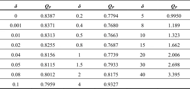
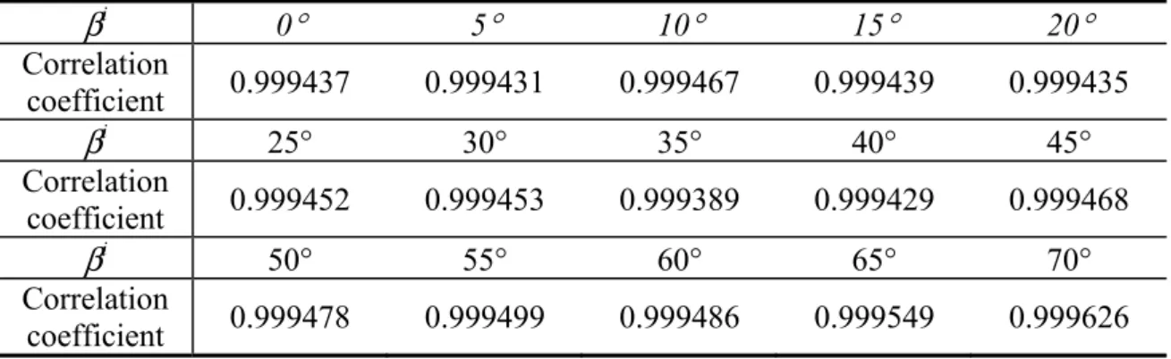
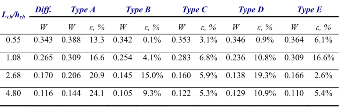
(9) List of Tables Table 2.3-1 Coefficients for interpolation formula (2.3-8)……………………………75 Table 2.3-2 Reduced flow rates vs δ…………………………………………………..75 Table 2.3-3 Pressure driven flow coefficient QP vs δ in case of square cross-section...75 Table 2.3-4 Temperature driven flow coefficient QT vs δ in case of square crosssection………………………………………………………………………….76 Table 3.1- 1 Software packages for molecular dynamic simulations…………………77 Table 3.5-1 Properties of graphic processing units used in current work [98]………...78 Table 3.5-2 Time spent for different procedures (in ms) by CPU (Intel Q9400) and by GPU (NVIDIA GeForce GTS250)……………………………………………..78 Table 3.5-3 Simulation time (in sec) of copper crystal on various GPUs versus number of atoms. System was simulated over 20000 time steps………………………..79 Table 3.5-4 Normalized time of execution of MD program on various computational systems………………………………………………………………………….79 Table 4.1-1. Correlation coefficients between <Ei> and <Es> for different angle of incidence βi……………………………………………………………………..80 Table 4.1-2. Coefficients A0 and B0 of the approximation polynomial (4.1-3)……….80 Table 4.1-3. Coefficients A1n,k of the approximation polynomial (4.1-4)……………..80 Table 4.1-4 Coefficients A2n,k of the approximation polynomial (4.1-6)……………...81 Table 4.1-5. Coefficients A3n,k of the approximation polynomial (4.1-7)……………..81 Table 4.1-6. Coefficients A4n,k of the approximation polynomial (4.1-8)……………..82 Table 4.1-7 Properties of wavy surfaces…...…………………………………………..82 Table 4.2-1 Flow rate through the channel versus the length-to-height ratio………….82 Table 4.2-2 Hydrodynamic conductance of the channel with various BCs on the walls………………………………………………………83 VII.

(10) Table 4.2-3 Gas flow rate through the channels with various BCs on the walls, length and pressure ratios……………………………………………………………...83 Table 4.2-4 Flow rate through various channels versus the length-to-height ratio……83 Table 4.3-1 Gas flow rate through the channels with various BCs on the walls. Parameters of simulations: P2/P1=1; T2/T1=500/350; δ=0.2……………………84 Table 4.3-2 Gas flow rate through the channels with various BCs on the walls………84. VIII.

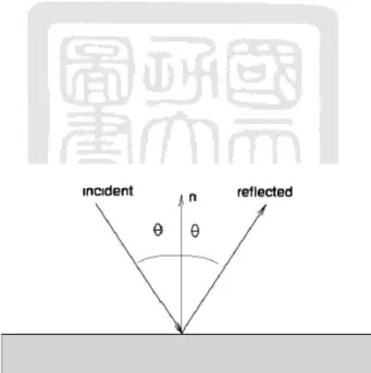
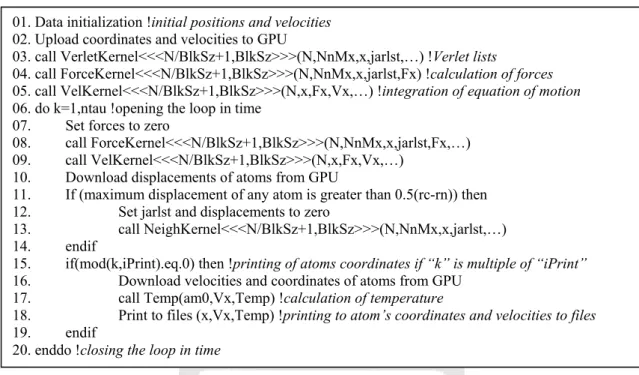
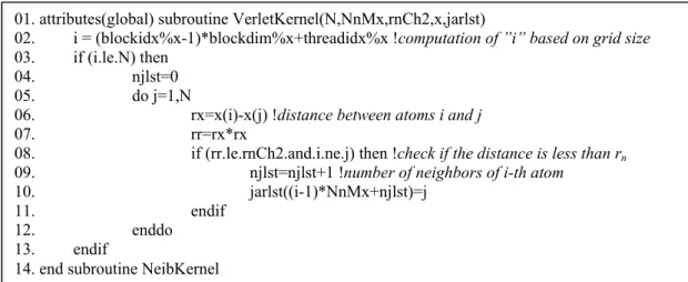
(11) List of Figures Figure 2.1-1 One stage of Knudsen compressor [64]………………………………….85 Figure 2.2-1 Sketch of the system used for simulations……………………………….85 Figure 2.3-1 Sketch of the 3D system used for theoretical analysis…………………...86 Figure 3.3-1a Sketch of specular reflection model…………………………………….86 Figure 3.3-1b Sketch of diffusive reflection model……………………………………87 Figure 3.3-2. Coordinate system……………………………………………………….87 Figure 3.3-3a. Sketch of tungsten channel used for simulations………………………88 Figure 3.3-3b. Side view of the channel with smooth and wavy walls………………..88 Figure 3.4-1. Lennard-Jones potential and force functions for argon…………………88 Figure 3.4-2. The Verlet list…………………………………………………………...89 Figure 3.5-1. Cubic unit of copper……………………………………………………..89 Figure 3.5-2 Pseudo code of OpenMP program……………………………………….90 Figure 3.5-3 Acceleration of MD program versus number of threads………………...91 Figure 3.5-4 Acceleration of “Verlet list” and “Forces” subroutines of MD program versus number of threads………………………………………………………91 Figure 3.5-5 Pseudo code of CUDA program…………………………………………92 Figure 3.5-6 Pseudo code of GPU’s subroutine for integration of equation of motion…………………………………………………………………………..92 Figure 3.5-7a Pseudo code of GPU’s subroutine for construction of neighbors lists……………………………………………………………….93 Figure 3.5-7b Pseudo code of GPU’s subroutine for construction of neighbors lists in case of Newton’s third law implementation……………………………………93 Figure 3.5-8a Pseudo code of GPU’s subroutine for Forces computations…………...94 Figure 3.5-8b Pseudo code of GPU’s subroutine for Forces computations…………...94 IX.

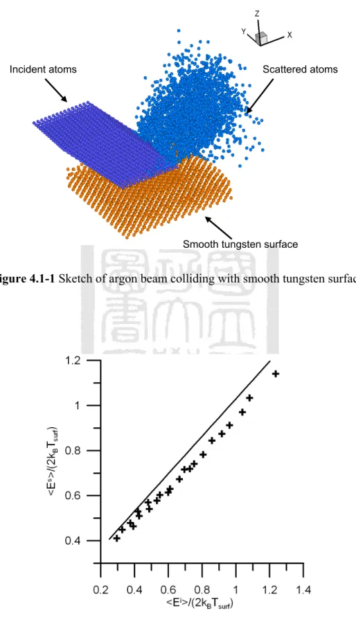
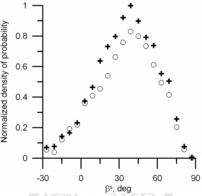
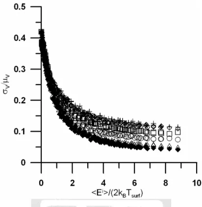
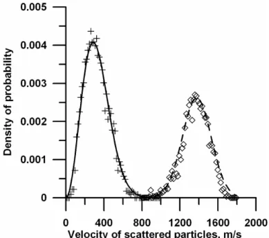
(12) Figure 4.1-1 Sketch of argon beam colliding with smooth tungsten surface…………95 Figure 4.1-2 Mean energy of scattered atoms versus energy of impinging atoms at β i =45°……………………………………………………………...95 Figure 4.1-3 Angular distribution of normalized probability density function in case of Ar scattering from W(110) at TG=295K and incident angle βi=45°………...…96 Figure 4.1-4 Mean energy of scattered atoms versus energy of impinging Ar atoms………………………………………………………………………96 Figure 4.1-5a Root mean square deviation of scattered atom’s velocities σV over mean velocity of scattered atoms μV versus kinetic energy impinging atoms………97 Figure 4.1-5b Root mean square deviation of scattered atom’s velocities σV over mean velocity of scattered atoms μV versus kinetic energy impinging atoms………..97 Figure 4.1-6 Density of probability of Vs. Tsurf=350K.………………………………...98 Figure 4.1-7a Normalized root mean square deviation σα of the azimuthal angle αs of scattered atoms versus kinetic energy of impinging atoms and incident polar angle…………………………………………………………………………….98 Figure 4.1-7b Normalized root mean square deviation σα of the azimuthal angle αs of scattered atoms versus kinetic energy of impinging atoms and incident polar angle…………………………………………………………………………….99 Figure 4.1-8a Normalized root mean square deviation σβ of the polar angle βs of scattered atoms versus kinetic energy of impinging atoms and incident polar angle…………………………………………………………………………….99 Figure 4.1-8b Normalized root mean square deviation σβ of the polar angle βs of scattered atoms versus kinetic energy of impinging atoms and incident polar angle…………………………………………………………………………100. X.

(13) Figure 4.1-9 Fraction of backscattered atoms versus energy of impinging Ar atoms…………………………………………………………..…………100 Figure 4.1-10a Average polar angle βs of scattered atoms versus kinetic energy of impinging atoms and incident polar angle………………………………….…101 Figure 4.1-10b Average polar angle βs of scattered atoms versus kinetic energy of impinging atoms and incident polar angle……………………….……………101 Figure 4.1-11 Correlation coefficients between βi and βs versus energy of incident beam………………………………………………………..………….………102 Figure 4.1-12 Density of probability of βs and αs. Tsurf=350K, βi=20°, Vi=100m/s…102 Figure 4.1-13 Density of probability of βs and αs. Tsurf=350K, βi=20°, Vi=1500m/s..103 Figure 4.1-14 Sketch of wavy surface………………………………………………..103 Figure 4.1-15 Fraction of atoms scattered by smooth tungsten surface in backward direction versus energy of impinging Ar atoms……………………………….104 Figure 4.1-16 Normalized root mean square deviation σα of the azimuthal angle αs of scattered atoms versus kinetic energy of impinging atoms and incident polar angle………………………………………………………………………..…104 Figure 4.1-17 Normalized root mean square deviation σβ of the polar angle βs of scattered atoms versus kinetic energy of impinging atoms and incident polar angle………………………………………………………………………..…105 Figure 4.1-18a. Density of probability of β s and α s . T s u r f =350K, β i =20°, V i =100m/s………………………………………………………………………….105 Figure 4.1-18b. Density of probability of β s and α s . T s u r f =350K, β i =20°, V i =1500m/s………………………………………………………………………..105. XI.

(14) Figure 4.1-19 Mean energy of scattered atoms versus energy of impinging atoms at. βi=45°…………………………………………………………………………106 Figure 4.1-20 Root mean square deviation of scattered atom’s velocities σV over mean velocity of scattered atoms μV versus kinetic energy impinging atoms………107 Figure 4.2-1 Reduced flow rate versus relative size of the tank……………………...107 Figure 4.2-2 Density of probability of velocity distribution of gas atoms in tank…...108 Figure 4.2-3a Normalized flow rate versus channel length-to-height ratio………….108 Figure 4.2-3b Normalized flow rate versus channel length-to-height ratio in a log-log scale…………………………………………………………………………...109 Figure 4.2-4a Normalized flow rate versus channel length-to-height ratio………….109 Figure 4.2-4b Normalized flow rate versus channel length-to-height ratio in log-log scale…………………………………………………………………………...110 Figure 4.2-5 Normalized flow rate versus pressure difference………………………110 Figure 4.3-1 Number of atoms in left (cold) tank versus time……………………….111 Figure 4.3-2a Normalized flow rate versus channel length-to-height ratio………….111 Figure 4.3-2b Normalized flow rate versus channel length-to-height ratio in log-log scale…………………………………………………………………………...112. XII.

(15) Nomenclature m - mass flow rate;. σ - root mean square deviation normalized by the root mean square deviation corresponding to a uniform distribution;. σμV - normalized root mean square deviation of scattered atom’s velocities; α=αS-αi – azimuthal angle change caused by the scattering of the beam; αi – incident azimuthal angle; βi – incident polar angle; αS - scattered beam’s azimuthal angle; βS - scattered beam’s polar angles; σV – root-mean-square deviation of the mean velocity of the atoms scattered by the surface;. μV - the mean velocity of the atoms scattered by the surface; <V> is the average molecular velocity; ∆P – pressure difference; ∆T – temperature difference; ∆t – time step; dch - diameter of the channel; DW- depth of the potential well of the Morse potential in case of tungsten-tungsten interactions; Ei – kinetic energy of the impinging atoms; ES – kinetic energy of the scattered atoms; H – height of a tank; hch – height of the channel;. XIII.

(16) J – gas flow rate; kB – Boltzmann constant; Kn – Knudsen number; Lch - length of the channel; m0 – mass of molecule of gas; N – number of gas atoms; n - number of molecules per unit volume; P – gas pressure; Pavg – average pressure; QP – flow coefficient in case of pressure driven flow; QT – flow coefficient in case of temperature driven flow; r – distance between atoms; rc – cutoff radius; rv – Verlet list radius; RW- width of the potential well of the Morse potential in case of tungsten-tungsten interactions; S – surface area; T – temperature; Tavg – average temperature; Tsurf – surface’s temperature; Vτi – tangential velocity component of the incident beam; VτS –tangential velocity component of the scattered beam. Vni – normal velocity component of the incident beam; VnS – normal velocity component of the scattered beam; vol – volume of a vessel;. XIV.

(17) Vx, Vy, Vz – velocity components in x, y, z directions, respectively; W – normalized flow rate; γ - Knudsen factor for thermomolecular pressure difference; δ - rarefaction parameter; λ – mean free path; μ – viscosity of the gas; μβ - average polar angle of the scattered atoms; ρ – density of the fluid;. XV.

(18) Chapter 1: Introduction 1.1 Motivation Improvements in microfabrication as well as falling prices due to this progress have grown the application area of microsystems, so that has motivated many engineers and researchers dealing with microchannels which are of significant parts for many micro-electro-mechanical-systems (MEMS). They have many ways of applications. Biochemical reaction chambers, heat exchanger and physical particle separators are also the possible applications. There is considerable interest in miniaturizing propulsion and power systems as well. While many miniature space and air breathing propulsion system concepts have been proposed [1], most of them require moving parts. All miniaturized propulsion devices with moving parts experience more difficulties with heat friction losses due to higher surface to volume ratios than their macroscale counterparts. Moreover sealing, fabrication and assembly are much more difficult at small scales because microfabrication processes have much poorer relative precision than convectional macroscale processes. Additionally, all air and space vehicles, regardless of size, require electrical power. The use of combustion processes for electrical power generation provides enormous advantages over batteries both in terms of energy storage per unit mass, as well as in power generation per unit volume, even when the conversion efficiency in combustion process from thermal energy to electrical energy is taken into account. Most current micro-scale power generation concepts employ scaled-down versions of existing macroscale devices. Particularly, microscale combustion engines have more problems with heat losses, friction, sealing, fabrication, assembly etc. compare to their macroscale counterparts.. 1.

(19) Recent advances in MEMS have made it possible to construct microscale sensors such as integrated gas chromatography systems, miniature spectrometers, and mass spectrometers. The miniaturized detection devices require microscale pumps to provide sensor elements with gas samples at necessary environmental conditions. There are two main ways to pump a gas: the first one is to impose a pressure gradient along the desired direction, this is a classical approach, but the significance of pressure driven flow decrease if gas becomes rarefied[2]. Another pumping mechanism that can be exploited in case of rarefied gas or microscale flow is thermal transpiration[3], a rarefied gas effect that drives gas flow along temperature gradient in a tube or channel. In some literatures, this effect is also called Knudsen effect. This phenomenon of low pressure gases (or gases in microscale systems) suggests that, by connecting two tanks with a very thin orifice or tube, one can transport a certain amount of gas from one to the other if the temperature gradient is set up along the tube. That is, the fine tube with a temperature gradient has a pumping effect. Based on above-mentioned effects, a novel compressor for a heat engine is proposed in [4], this device works on the basis of the thermal transport of gas according to the Knudsen effect. Such pressure generator is usually called Knudsen compressor[59], this device has very attractive advantages: •. There are no moving parts, consequently such compressor don’t need any lubricants or other liquids;. •. It can operate on waste heat from other equipment;. •. It can operate over a wide range of pressures; The main disadvantage is low mass flow rate and efficiency. However, this. disadvantage becomes unimportant in case of operating on waste heat. 2.

(20) In fact, many devices based on rarified gas flow surround us everyday. One of them is a hard disk Drive. Pressure inside the hermetic box with disks is about atmospheric, but the distance between reader head and platter is around 50nm. The gas flow between the header and platter can be considered as nanoflow with both temperature and pressure instabilities, consequently temperature driven flow might occur. From scientific points of view, studies of Knudsen compressor can provide the detailed information about gas-gas and gas-surface interactions in temperature driven flow to verify kinetic models. From the practical points of view, this effect can be used in gas separation [10-13]. Knudsen number (Kn) allows us to judge whether flow is continuum or not. The Knudsen number is a dimensionless number defined as the ratio of the molecular mean free path length to a physical characteristic length scale. This characteristic length scale is based on physical system. It could be, for example, radius of a nano-channel in a Knudsen compressor. If the Knudsen number is near or greater than one, the mean free path of a molecule is comparable to the characteristic length scale of physical problem, and the continuum concept in conventional fluid mechanics is no longer a good assumption. In this case statistical physical model must be used. Generally speaking, temperature driven flow is an important issue if one deals with rarefied gases (or gases in microscale devices), which must be studied as detailed as possible. One way of study is experimental approach, but it is well known that good experiments are expensive, also it should be noted that sometimes experiments cannot provide full data due to the scale limitations, for example it is complicated to measure flow field of micro- or nanoscale flow. Another way of a studying is computer. 3.

(21) modeling. That kind of studying has a lot of advantages, such like: low amount of involved facilities (usually it is just one computer); computer model is very flexible i.e. it allows studies of different properties without serious changes inside the model. One of the most popular methods for rarified gas simulation is Molecular Dynamic (MD) method[14]. This method is based on the first principles of mechanics and it can provide detail information about each molecule (atom) behavior. Sometimes, this simulation method is called “numerical experiments”.. 1.2 Phenomenon background The implementation of pressure driven flow is straightforward: what one needs is to impose a pressure difference and the fluid starts flow in direction of pressure gradient, but let’s discuss the mechanism of pressure driven flow on molecular level. First of all, let’s consider the simplest case of gas flow from reservoir into vacuum through an orifice. In this case, flow rate of rarefied gas through small orifice is equal to number of molecules colliding with the surface per unit time and per unit surface area. Consider a surface area of the wall, S, and a molecule which impinges on the wall with x-component of velocity, Vx within a small time interval Δt. In the time Δt, the molecule will travel a distance VxΔt in the x-direction. (Let Vx be positive so that the molecule is traveling in the +x direction.) The molecule will hit the wall in the time Δt if it lies within a distance VxΔt from the wall. This distance multiplied by the area, S, creates a small volume SVxΔt. If the number density of the gas is N/vol, this small volume contains molecules: N SVx Δt vol. The number of these molecules which have velocity, Vx, is. 4. (1.2-1).

(22) N N SVx Δtf (Vx ) dVx = S ΔtVx f (Vx ) dVx , vol vol. (1.2-2). where f(Vx) is Maxwell-Boltzmann distribution for velocity in x-direction: f (Vx ) =.  − m0Vx 2  m0 exp   2π k B T  2k B T . (1.2-3). Then the total number of collisions is obtained by summing this number of collisions over all positive Vx (summation in this case, of course, means we integrate over Vx from 0 to ∞), ∞ Vx N N S Δt  Vx f (Vx ) dVx = S Δt vol vol 2 0. (1.2-4). In Equation (1.2-4) we have used the definition of the average of the absolute value of Vx, Vx =. ∞.  V f (V ) dV x. x. (1.2-5). x. −∞. and the fact that |Vx|f(Vx) is an even function of Vx, so that,. Vx =. ∞.  V f (V ) dV x. −∞. x. x. ∞. ∞. 0. 0. = 2 Vx f (Vx ) dVx = 2 Vx f (Vx ) dVx. (1.2-6). So, to find the number of collisions per unit time per unit area, we divide the number of collisions in Equation (1.2-4) by the area and by the time interval, Δt. Vx N S Δt collisions vol 2 = S Δt S Δt. 1 N Vx 2 vol. (1.2-7). 1  1 V = V , 2 2. (1.2-8). =. Taking in account that: Vx =. 5.

(23)  where V = V = Vx 2 + Vy 2 + Vz 2 . Finally we have: collisions 1 N 1 N  1 N 1 = Vx = V = V = n V = J0 S Δt 2 vol 4 vol 4 vol 4. (1.2-9). The last expression allows us to estimate the flow rate of rarefied gas through orifice into the vacuum. The net flux in case of two vessels connected by a tiny hole is results of superposition of two fluxes:. J12 = J 01 − J 02 ,. (1.2-10). where J01 and J02 are the flow rate of gas exhaust from first and second tank toward vacuum, respectively. It should be noted that the flux J could be driven by pressure gradient, as well as by temperature gradient in case of non-isothermal flow. The impact of pressure driven flow component to the net flow rate is inversely proportional to Knudsen number [15]. Meanwhile the temperature driven flow component becomes significant in case of rarified flow conditions. Temperature driven flow of rarefied gas arises if vessels are connected by orifice or channel with longitudinal temperature gradients. In this case the fluid starts creeping in the direction from cold end toward hot end. This is so-called thermal creeping or transpiration phenomenon. We will explain this counterintuitive effect with the following example. Consider two tanks filled with the same gas that are kept at the same pressure (P1=P2), but at different temperatures (T1>T2). If these two containers are connected with a relatively large channel (λ<<hch), no flow occurs in the channel. If the channel’s. 6.

(24) height (hch) becomes comparable to the mean free path (λ), rarefied gas effects have to be taken in account. In such a case the local equilibrium mechanism is very complex, and interaction of gas molecules with the walls must also be considered. Here, we consider free molecular flow conditions (λ>>hch) to simplify discussion. In this flow regime, intermolecular collisions are negligible compare to the interactions of molecules with surfaces. Let us assume (for simplicity) that molecule-wall interactions are specular (gas is ideal), then the following analysis is valid. One can assume that the density of the fluid is proportional to the number of molecules per unit volume, ρ~n, and temperature of fluid is proportional to square of average molecular speed, T ~ V. 2. . The mass fluxes at hot and cold ends of the channel are m0 n1 V1 and m0 n2 V2 , respectively, here m0 is the mass of one gas molecule. Then. m0 n1 V1 ρ T  ≈ 1 1 m0 n2 V2 ρ 2  T2 . 0.5. P T  = 1 2 P2  T1 . 0.5. (1.2-11). where the equation of state is used as: P = ρ RT. (1.2-12). The following equation is the Knudsen relation for the equilibrium state (in equilibrium state the net mass flux between the vessels is zero, i.e. m0 n1 V1 = m0 n2 V2 ): P2 P = 1γ , γ T2 T1. (1.2-13). where γ is a Knudsen factor for thermomolecular pressure difference; in case of ideal gas and thin orifice γ=0.5. The above analysis indicates a flow creeping from cold to. 7.

(25) hot, but it should be noted that equations(1.2-9) and (1.2-13) have been obtained with ideal gas assumption[16].. 1.3 Research Objectives In this study, molecular dynamics (MD) method was used for investigation of collision of argon atoms with tungsten surface and rarefied gas (Knudsen number greater than one) flow through the micro- and nano- channels. The objectives of this work are the following: 1. To find the appropriate physical model that is simple enough to be implemented using MD method, but at the same time it is able to reproduce all processes accompanying pressure and temperature driven flows of rarefied gas; 2. To investigate the degree of influence of gas-surface interactions on parameters of flow and check the applicability of widely used Maxwell boundary conditions in case of simulations of pressure- and temperature-driven flow; 3. To find a suitable solution of the main problem of MD simulations – time consumption; 4. To investigate pressure- and temperature-driven flows of rarefied gas through micro- and nano-channels with various boundary conditions;. 1.4 Literature review Micro- and nano-channels are widely used nowadays, examples can be easily found in medicine, biotechnologies, telecommunication and etc. The most obvious application for nano-channels is gas separation[10-13]. The specific examples of devices related to micro flow are inkjet printheads, microchannel-based chemical. 8.

(26) reactors, pressure sensors, micro total analysis system(μTAS) or "lab on a chip", micropumps, and Knudsen pumps [17]. Investigation of rarefied gas caused by temperature and pressure gradient as basis of a vacuum pump has been a long history since the early 1900s. The phenomenon of temperature driven flow was first explained by Reynolds[18] and contemporaneously investigated theoretically by Maxwell[19]. In early 1909 Martin Knudsen has published paper[20] dealing with molecular flow and effusion through orifices. This study introduces the idea of treating flow as impedance in the electrical sense so that one could derive a combination of a tube and an orifice in terms of their flow resistance summation. This idea was supported by Dushman [21] who stated that the flow resistance of a long tube is the sum of the resistances of the entrance opening and that of a short tube. In 1932 Clausing has introduced the concept of transmission probability on preference to flow resistance (or conductance)[22]. Further evaluation of transmission probabilities was conducted by De Marcus and Hopper to obtain approximate solutions to the Clausing-type integral equations[23]. Development of computers has allowed one to implement another useful approach, particularly well-suited for complex shapes and systems of baffles, traps, etc, is the statistical one using Monte Carlo techniques. This was described by Davis[24] and many publications since then. One of the earliest experimental studies of gas flow through copper membrane has been conducted by Warrick and Mack [25] in 1933. Hanks and Weissberg [26] have proposed semi-empirical equation for the pressure driven flow through a circular channel. This relation was recently tested by Shinagawa et al.[27] and it was found to be valid in the range of the continuum to the upper limit of transition regime.. 9.

(27) In 1973 Borisov et al. [28] have studied dependence of thermomolecular pressure difference on the average pressure. Experimental studies have been conducted for different gases (He, Ne, H2 and D2) in the continuum flow regime. Researches have experimentally proven that in the continuum flow regime the value of factor γ in eq. (1.2-13) tends toward zero. Results are in line with theoretical studies by Sone et al. [29]. Fujimoto and Usami [30] have reported the experimental studies of gas flow through orifices or short channels over the entire flow regime from continuum to free molecular. Unfortunately all experiments have been carried out for the case of high pressure difference and most results are shown in figures that allow only quantitative comparison. Sreekanth [31] has conducted experimental studies of rarefied gas flow through short metal nano-channels in a wide range of pressure ratios. That paper proposes semi-empirical equation for estimation of mass flow rate:  π d ch 4 P1 + P2 0.519d ch3  1 , m =  ΔP +  V1 2 128μ RT1  Lch (1 + d ch / Lch ). (1.4-1). where <V> is the average molecular velocity; μ – viscosity of the gas; P and T are the pressure and temperature of the gas, respectively. Variables with subscripts 1 and 2 correspond to the parameters of gas in the upstream and downstream reservoirs. This relation was obtained for the case of transition flow through the extremely short tubes (Lch/dch<1 length to diameter ratio). Works by Johnsen and Chatterjee [32] deal with experimental studies of binary gas mixtures flow through a small thin orifice (thickness ~10% of diameter); a limited range of the transition regime from molecular to continuum flow has been covered. The observed density changes of gas species are found to depend strongly on the mass ratio. 10.

(28) of the two flowing gases. Authors have derived a semi-empirical formula that estimates the density changes. Recently Marino [33] has carried out experiments in order to evaluate the conductance of tubes of circular cross section as a function of Knudsen number. The main impact of this study is tabulated data of conductance of long tubes. The results discussed in this manuscript have good correlations with theoretical [34] and experimental [31] studies by other researches. Setup of good experiments related to rarefied gas flow through micro- or nanochannels is very expensive and time consuming issue, but sometimes experiments has problem with no appropriate solution. The complicity is caused by spatial resolution since measurement in a nano-channel with lengthscale 10-9m requires a sensor with 1010. m scale at least. Another problem is that sensor measurements are sensitive to. disturbances. Therefore, it is impossible to put a probe inside a micro-channel to measure velocity, temperature or pressure field directly. All this issues create obstacles on the way of obtaining reliable information about micro- and nano-flows. Fortunately, recent achievements of mathematics, numerical simulation methods and computer science allowed us to investigate all these tiny effects in a wide range of parameters of interest. It is obvious that flows through membranes are more interesting from the practical point of view, but theoretical study of such complicated systems is very sophisticated. Commonly numerical or analytical investigation of gas flows through the membrane are performed considering single channel or small set of parallel channels with further extrapolation of results to the case of membrane using correction factors [35].. 11.

(29) There are a lot of studies using both temperature and pressure driven flows through long channels, for example works by Sharipov [36]. This paper is related to calculations of the mass flow rate of a rarefied gas through a long capillary caused by small pressure and temperature gradients based on the s-model (a generalization of the Bhatnagar-Gross-Krook model [37], see for example [38]) for the diffuse specular gassurface interaction in the range of the rarefaction parameter δ (δ~1/Kn) from 0.005 to 50. Author of Ref.[36] has determined that the nonlinear thermomolecular pressure difference does not depend on the shape of temperature distribution along the capillary in case of free molecular flow regime. The nonlinear thermal creep has been calculated for two different temperature distributions (linear and nonlinear) along the capillary. It has been shown that the application of the linear theory (this theory is based on the assumption of constant values of flow coefficients along the channel) to the gas flow at a large temperature ratio gives a significant error. Another work by Sharipov [39] was concentrated on research of rarefied gas flow through a long rectangular channel caused by both pressure and temperature differences. Author has proposed equations that allow one calculate a mass flow rate through a long rectangular channel. It was pointed out that the numerical results on pressure driven flow can be used for any type of gas, including polyatomic, while the data on the thermal creep can only be used for monoatomic gases. The thermal creep must be recalculated for any specific polyatomic gas by applying an appropriate kinetic equation. Unfortunately author of the last two works proposed relations for a long channel without specification of the “long” term, thus it is to be determined. Shen et al. [40] have simulated rarefied gas flows through micro-channels using information preservation method (IP) and the direct simulation Monte Carlo (DSMC) method. This study deals with stream-wise pressure distributions and mass fluxes through micro-channels given by IP method agree well with. 12.

(30) experimental data measure in long micro-channels by Arkilic et al. [41]. It was found that IP and DSMC calculations are able to represent flow behaviors through short micro-channel over the entire flow regime from continuum to free molecular, whereas the slip Navier-Stokes solution fails to predict it. Paper [15] represents comprehensive numerical study of a gas flow through a long pipe with elliptic cross section. The flow considered in the work is non-isothermal, and all computations have been performed for the cases of small temperature and pressure gradients along the channel. All parameters of interest are studied on the basis of Smodel kinetic equation. The main result on this work is proposed a data set which relates dependence between rarefaction parameter and non-dimensional flow rate. Additionally this work proposes the relation allows one to compute both temperature and pressure driven flow for the cases with large gradients. Titarev and Shakhov [42] have developed a conservative numerical method for solving the linearized S model kinetic equation. The method is intended for channels with an arbitrary cross section in the entire range of Knudsen numbers. The gas flow rate for a channel cross section specified in the form of a regular polygon was numerically computed in a wide range of rarefaction parameters. Investigations have been performed for the case of infinite channel. It was shown that the solution of the problem converges quadratically in the number of cross section sides to the limiting case of a circular pipe. The main result is that for triangular and quadrilateral cross sections, the mass flow rates and the heat fluxes were found to differ substantially from the case of a circular pipe. On the other hand the gas flows through extremely short channels (slits and orifices) have been intensively studied as well, see for example work of Lilly et al. [43].. 13.

(31) Efforts of the authors were mainly concentrated on determination of propulsion properties of orifices and short channels (thick orifices). It has been found that the effect of surface secularity on a thick orifice specific impulse was found to be relatively small. Authors of works [44-46] have done analytical and numerical studies of rarefied gas flow through slits and orifices of different shapes. Non-isothermal gas flow is discussed [44]; They proposed equations allow one to estimate flow rate of temperature driven flow through slit over a wide range of Knudsen number. Research described in [45] represents studies of 2D rarefied gas flow through the thin slit into the vacuum by using the BGK and S-model equations. The obtained results have good agreement with similar studies performed using DSMC method. This paper presents numerical data on the flow rate and distributions of density, bulk velocity and temperature along the symmetry axis. According to the results listed in the paper, the mass flow rate increases with the increase of rarefaction parameter, and it reaches a constant value when the flow regime becomes continuous. Rarefied gas flow between two containers through a thin slit is studied on the basis of the direct simulation Monte Carlo method [46]. The flow rate and flow field are calculated over the whole range of gas rarefaction for various values of the pressure ratio. It is found that at all values of the pressure ratio a significant variation of the flow rate occurs in the transition regime between the free-molecular and continuum regimes. DSMC method has been widely used for investigations of rarefied gas flow through micro- and nano-channels, for example [15, 34, 47-50]. Varoutis et al. have investigated pressure driven flow through a long circular pipe [48]. This work covers wide range of flow regimes (rarefied flow and continuum flow, flow to the vacuum and flow between two containers with different pressures) through the different types of channel (L/R was. 14.

(32) varied from 0.1 to 10). It has been found that the rarefaction parameter has the most significant effect on the flow field characteristics and patterns, followed by the pressure ratio drop, while the length-to-radius ratio has a rather modest impact. Several interesting findings have been reported including the behavior of the flow rate and other macroscopic quantities in terms of these three parameters. In addition, the effects of gas rarefaction on the choked flow at large pressure drops is discussed. In contrast to the previous papers, the work [34] describes studies of rarified gas flow through short tubes into vacuum. Authors used DSMC method to investigate the phenomenon of interest. The intermolecular potential was modeled using the hardsphere (HS) and the variable hard sphere (VHS) models. Computations are performed for various L/R ratios and rarefaction parameters. It has been shown the mass flow rate is strongly sensitive to the choice of gas-surface interaction model, meanwhile the intermolecular potential does not influence on the flow rate significantly. Results described in this paper have been supported experimentally by Marino [33]. Almost all studies mentioned above have been conducted using kinetic model or DSMC method, it should be noted that there is a relatively new method simulation technique for complex fluid systems called Lattice-Boltzmann method (LBM). Instead of solving Navier–Stokes equations, the discrete Boltzmann equation is solved to simulate the flow of Newtonian fluid with collision models such as Bhatnagar-GrossKrook (BGK). This method has been successfully applied for the investigation of micro and nano-channel flow[51]. The paper by Ghazanfarian and Abbassi [52] deals with two-dimensional numerical simulation of gaseous flow and heat transfer in planar microchannel and nanochannel with different wall temperatures in transitional regime 0.1<Kn<1. An. 15.

(33) atomistic molecular simulation method was used known as thermal lattice-Boltzmann method. The simulation results of thermal lattice- Boltzmann method in the described study shows that this method is capable of modeling shear-driven, pressure-driven, and mixed shear–pressure-driven rarified flows and heat transfer up to Kn=1 in the transitional regime. Taguchi and Charrier [53] have studied steady rarefied gas flow through periodic porous media kept at an uniform temperature. It was considered on the basis of Bhatnagar–Gross–Krook equation with the diffuse reflection condition on the solid boundary. Authors have derived, by homogenization, a fluid model that describes the global pressure distribution as well as the mass-flow rate. The derived model has a simple form and can be used as a practical tool. A simple application of the derived model to an isothermal flow through an array of circular cylinders induced by a pressure difference is presented Despite the increasing popularity of LBM in simulating complex fluid systems, this novel approach has some limitations. At present, high Mach number flows in aerodynamics are still difficult for LBM, and a consistent thermo-hydrodynamic scheme (scheme that couples heat and mass transfer processes together) is absent. However, as with Navier–Stokes based CFD, LBM methods have been successfully coupled to thermal-specific solutions to enable heat transfer (solids-based conduction, convection and radiation) simulation capability. For multiphase/multicomponent models, the interface thickness is usually large and the density ratio across the interface is small when compared with real fluids. Nevertheless, the wide applications and fast advancements of this method during the past twenty years have proven its potential in computational physics, including microfluidics: LBM demonstrates promising results in the area of high Knudsen number flows. Sbragaglia et al.[54] have specialize the 16.

(34) Boltzmann kinetic equation to describe the wetting/dewetting transition of fluids in the presence of nanoscopic grooves etched on the boundaries. This approach permits one to retain the essential supramolecular (it is well defined complex of molecules held together. by. noncovalent. bonds). details. of. fluid-solid. interactions. without. surrendering—actually boosting—the computational efficiency of continuum methods. The method is used to analyze the importance of conspiring effects between hydrophobicity and roughness on the global mass flow rate of the microchannel. The mesoscopic method was also validated quantitatively against the molecular dynamics results by Cottin-Bizonne et al. [55]. Molecular Dynamics method is a simulation approach based on fundamental laws of mechanics that allows one consider behavior of every single atom/molecule of system of interest. In contrast to DSMC, it allows one to describe non-equilibrium processes, moreover MD method is able to reproduce complex mixtures of gases and/or liquids, while the LBM method experiences some problems in this case. Mi et al. [56] have applied MD simulations to study nanochannel flows at low Reynolds numbers. A simple fluid flowing through channels of different shapes at nanoscale level is investigated. Comparing velocities and other flow parameters obtained from MD simulations with those predicted by the classical Navier-Stokes equations at same Reynolds numbers, researchers found that both results agree with each other qualitatively in the central area of a nanochannel. However, large deviation of flow field usually exists in areas near the wall. For certain complex nanochannel flow geometry, MD simulations reveal the generation and development of nano-size vortices due to the large momenta of molecules in the near-wall region while the traditional Navier-Stokes equations with the non-slip boundary condition at low Reynolds numbers cannot predict. 17.

(35) the similar phenomena. It is shown that although Navier-Stokes equations are still partially valid, they fail to give whole details for nanochannel flows. Okumura and Heyes [57] have compared the results of three-dimensional MD simulations of a Lennard-Jones (LJ) liquid with a hydrostatic (HS) solution of a high temperature liquid channel which is surrounded by a fluid at lower temperature. Because the systems were in stationary non-equilibrium states with no fluid flow, both MD simulation and the HS solution gave flat velocity profiles for a normal pressure in all temperature-gradient cases. However, the other quantities showed differences between these two methods. The MD-derived density was found to oscillate over the length of 8 LJ particle diameters from the boundary plane in the system with the infinite temperature gradient, while the HS-derived density showed simply a stepwise profile. The MD simulation also showed another anomaly near the boundary in potential energy. Authors have found systems in which the HS treatment works well and those where the HS approach breaks down, and therefore established the minimum length scale for the HS treatment to be valid. Molecular dynamics-continuum hybrid simulation method has been proposed by Sun et al.[58] for studies of influence of roughness and thermal boundaries effect on flow in microchannel/nanochannel. The results indicate that the molecules in the wallneighboring area can be firmly confined in the concaves due to geometric structure and strong liquid–solid interaction and cause locking boundary in the velocity profile and linear gradient in the temperature profile. The locked boundary can further lead to negative slip length, which varies in power law with channel height. Authors of the Ref. [58] have sown that the linear temperature gradient, as well as nearly constant temperature jump, can lead to obviously increasing Kapitza length (Kapitza length. 18.

(36) represents the length of a material of a given thermal conductivity providing an equivalent thermal resistance as the interface[59]) versus channel height. When using the molecular dynamics simulation method to study low speed nanoscale flow problems, a major difficulty is the extraction of the true flow velocity because of the highly nonlinear coupling of the low bulk flow velocity and the high velocity of molecules’ thermal motion. In all published papers the reported flow velocity is the average value of the sum of these two velocities over time. For high speed flow problems the conventional MD method can give satisfactory result. However, when the flow velocity is much smaller than the thermal velocity, the conventional molecular dynamics simulation method cannot predict the true flow velocity. To overcome this difficulty, Zhang et al. [60] have developed a new linearized algorithm. The new algorithm separates the flow velocity increment caused by external forces from the thermal motion velocity at each time step. The detailed process of the new algorithm is derived in the paper and several cases of 3D nano-channel flows of liquid argon are simulated by using this method. The numerical results show that the new algorithm is valid for nanoscale flows. From the analysis of the entire set of the discussed experimental and theoretical studies we can draw some final comments. There are a lot experimental studies of rarefied gas flow, but unfortunately most of them do not provide results in a manner that can be used for comparison and analysis. Despite the number of existing numerical studies we can say that most of them are related to two limiting cases: extremely short channels (orifices) or long channels, while the middle-size channels are almost undiscussed. Another important issue is boundary conditions (BC), most of papers mentioned above deal with diffusive or specular diffusive BC. Such boundary conditions are not fully valid for all cases of interactions of gas molecules with clean 19.

(37) metal surface [61]. It should be noted that this model of BC can results in wrong estimations of non-isothermal flow though mico- nano-channel [2]. We can say that rarefied flow in tubes of different length-to-diameter ratio still represents an interesting and not fully investigated field. The importance of the research in this area is enhanced by the recent increasing technological applications.. 1.5 Research procedure First of all, the relevant literature was collected and reviewed in order to identify background, history, current trends and recent results of investigations on micro- and nano-flows and models gas-surface interactions. The studying model of micro channel was designed, one should keep in mind that described model in this thesis is quite ideal. Then the mathematical approach was formulated: Molecular Dynamic method with second order Verlet integration of equations of motion and four types of boundary conditions were used during this investigation. Base on the chosen physical model and mathematical approach the program code was created using the Fortran language and parallel programming technologies. After obtained results were analyzed and discussed.. 1.6 Thesis Outline •. Chapter 1 explains motivations of current research work. Rarefied gas flow background is provided in this chapter. The introductory chapter also outlines objectives and structure of this thesis. Literature review, perspective ways of application are presented in this chapter. 20.

(38) •. Chapter 2 introduces model, which was used for current investigations are presented in this chapter.. •. Chapter 3 provides detailed information about mathematical approach, which was used for the investigation. Boundary conditions, initial conditions and interatomic interaction conditions are described in Chapter 3.. •. Chapter 4 represents data collection and describes results obtained during the simulations.. •. Chapter 5 then summarizes the data of the simulations and provides some conclusions based on obtained results.. 21.

(39) Chapter 2: Physical model description 2.1 Concept of the model The best way to investigate a natural process is to observe it as it is. This approach gives whole picture of the ongoing processes, but on the other hand it doesn’t allow the researches to differentiate and control the order of impact of ambient conditions on the observed process. This issue might cause the wrong conclusions about the dependences between studied process and side forces influencing on it. Consequently, every good experimental study requires definition of parameter set that are assumed to be important for the process of interest. If the model is too simple, it might not be able to reproduce the natural process. However, the excess of included conditions may lead us to a problem with many unknowns which become too complicated to be solved or analyzed. Considering real micro- and nano-flows, one can see that real flows involve complex gas mixtures and channels with nonuniform geometry. The good examples of these flows are blood flow in lung capillaries[62], flows through sponges or aerogels [63]. It should be noted that micro scale flows of gases are similar to high altitude flow around parts of flying vehicle – molecular interactions plays important role and methods of continuum fluid analysis are not fully valid in those cases. In contrast to experimental dealing with dense flow, studies of high Knudsen number flow are limited by number of tools. For example, the streamlines in case of low Kn number can be visualized using PIV techniques, but this approach is useless in case of rarefied flow. Moreover, measurement of temperature and pressure field requires very accurate sensors that cause experiment expensive significantly. The common model in case of rarefied gas mico-flow usually consists of a channel or slit connected to source of working fluid. Mainly, there are only few parameters that can be directly. 22.

(40) measure in case of rarefied gas flow: inlet/outlet pressure and temperature; mass flow rate. Velocity profile can be measure in some cases related to transient flows. The main advantage of numerical simulations is able to provide almost any desired parameters. In fact, recent advantages of numerical methods and computer science allow one to simulate a very complex system. It is possible to simulate the flow inside pores of a membrane. However, numerical simulation is usually limited by amount of RAM memory and quality/quantity of available CPUs. If the system is too complex, simulation will require a lot of computer resources and time. The good example of suitable model for rarefied gas flow investigations was proposed by Muntz and Vargo [64]. It is illustrated in Figure 2.1-1. In fact this model was used to deal with Knudsen effect, but the concept can be used for other studies of rarefied gas flow. Each stage has a membrane section where temperature increases, causing the pressure increases due to the rarefied gas phenomena of thermal creep or thermal transpiration. Temperatures of cold and hot tanks are T1 and T2 respectively, Lxi - length of capillary section of i stage, LXi - length of connector area of i stage. The direction of the thermal creep flows inside the membrane channels is from cold to hot (thus left to right in Figure 2.1-1). A return flow, caused by the induced pressure gradient, creates a flow from the hot end to the cold end of the membrane (right to left in Figure 2.1-1). Following the membrane section, there is a connector section with a significantly larger radius than the individual capillaries. In multistage compressor, a linear temperature decrease is also imposed along the horizontal wall of the hot-side connector section. This is to ensure that, at the exit from the hot-side connector, the working gas has returned to the same temperature when it entered the stage. Such temperature distribution contrasts to the temperature distribution in single stage Knudsen compressor, which has temperature gradient just along the capillaries. 23.

(41) It should be realized that model described above it just a mathematical view of studied device. Real compressor is sophisticated construction composed of a vast number of parts, also real device is not single stage, because one stage has very low efficiency.. 2.2 Current model description Model discussed in present work was based on previous studying of Muntz[64] and Alexeenko[47]. Current three-dimensional model is presented in Figure 2.2-1. This system consists of two rectangular tanks filled with argon with values of pressure and temperature of P1, T1 and P2, T2, respectively. The argon flows between tanks through the channel of square cross-section attached to the tank’s wall. We have found (see section 4.2) that the lateral dimensions of the tank must be at least 4 times greater that the corresponding sizes of the channel (H/hch≥4); it guarantees that flow properties are not affected by the boundaries of the vessel. The pressure in both vessels was maintained at a constant value by adding new gas atoms to the left quarter of the tank, in case of the left tank, and to the right quarter – in case of the right one. Specular BC are set up on the 5 faces of each tank, while the leftmost and the rightmost faces (ABCD and EFJK) are free interface boundaries, i.e. gas atoms are allowed to migrate through them. Atoms that passed through the plane ABCD or EFJK were excluded from the simulation. It should be noted that models used for current study are ideal models having the following assumptions:. •. Walls of tanks are modeled as solid and ideal (without any irregularity and scratches), and the walls do not have any molecular/atomic structure;. 24.

(42) •. Size of lateral side of tanks is 8 times greater than corresponding dimension of channel;. •. The working gas is 100% pure Argon;. •. Tanks were initially filled just by gas – channel was empty;. •. Gravity force, or any another external force field, does not exist. Due to this assumption, gas particles have the same probability to reach any point of space no matter how tanks are arranged;. •. Gas does not react chemically with surfaces of device.. These properties are common for all cases studied in current work.. 2.3 Theoretical analysis Equations (1.2-9) and (1.2-10) allow one to perform analysis of flow through the orifice (Lch/hch=0) connecting two tanks filled by gas (Figure 2.3-1). From the engineering point of view, it is very difficult to create infinitely thin rigid wall with one hole. But the theoretical expressions shown below allow one judge whether numerical model is able to reproduce physical processes related to rarefied gas flow or not. Following two cases will be used to check the correctness of current numerical simulation. The first case: total number of enclosed atoms is constant (N=N1+N2=const); tanks are of equal size; flow is isothermal T1=T2. Rate of change of number of gas atoms in left tank (Figure 2.3-1) N S dN1 N = J 2 − J1 =  2 V2 − 1 V1  dt vol1  vol2 4. Integration of eq. (2.3-1) gives:. 25. (2.3-1).

(43)   V V  V   V V S ln −  2 + 1  N1 + N 2  = −  2 + 1  t + ln C1 vol2   vol2 vol1  4   vol2 vol1 . (2.3-2). Constant C1 can be determined using initial condition: N1(t=0)=N10  V V  V V V C1 = −  2 + 1  N10 + N 2 = ( N − N10 ) 2 − 1 N10 vol2 vol2 vol1  vol2 vol1 . (2.3-3). Substitution of C1 in (2.3-2) gives:   V V  V  ln −  2 + 1  N1 + N 2  = vol2    vol2 vol1   V V S  V V  = −  2 + 1  t + ln ( N − N10 ) 2 − 1 N10  vol2 vol1  vol2 vol1  4    V V  V −  2 + 1  N1 + N 2 = vol2  vol2 vol1    V   V V V  S  = ( N − N10 ) 2 − 1 N10  exp −  2 + 1  t  vol2 vol1   vol2 vol1  4   . (2.3-4). (2.3-5). Number of gas atoms in left tank versus time:. N1 ( t ) =. V2 V V2 − 1 N10   V V  S  vol2 vol1 vol2 exp −  2 + 1  t  + (2.3-6) V1   V2   vol2 vol1  4  V2 + V1 − +  vol2 vol1  vol2 vol1 . ( N − N10 ). If the flow is isothermal and tanks are of equal size and all gas was initially stored in the left tank, then the eq. (2.3-6) becomes: N1 ( t ) =.  V S  N N exp  − t + 2  vol 2  2. (2.3-7). Equations (2.3-6) and (2.3-7) allows one to estimate the rate of change of number of gas atoms in tanks. Expressions mentioned above are valid in case of rarefied gas (δ<1),. 26.

(44) while in case of continuum regime parameters of flow become sensitive to rarefaction degree and shape of orifice as well [15]. Authors of [46] have proposed and equation that relates dimensionless flow rate with pressure drop and rarefaction parameter δ practically for the whole range of gas rarefaction:  P  Aδ − Bδ ln δ + Cδ 2 W = 1 − 2  1 + P1   1 + Dδ + Eδ 2 .  , . (2.3-8). where the interpolating coefficients are given in Table 2.3-1. The second case: initially pressures in both tanks were equal; tanks are of equal size; flow is not isothermal T1<T2. Rate of change of number of gas atoms in left tank: V V S dN1  =  N 20 2 − N1 1  dt vol2 vol1  4 . dN1. (2.3-9). N. t. 1 dN1 S S = dt →  =  dt V V V V 4 4 N10 0 N 20 2 − N1 1 N 20 2 − N1 1 vol2 vol1 vol2 vol1. (2.3-10). Initial number of gas atoms in the left tank: N1(t=0)=N10  V V  ln  N 20 2 − N1 1  vol2 vol1  −  V1 vol1. N1. =. S t 4. N10.  V V   V V  V S ln  N 20 2 − N10 1  − ln  N 20 2 − N1 1  = 1 t vol2 vol1  vol2 vol1  vol1 4  . Number of gas atoms in left tank versus time:. 27. (2.3-11). (2.3-12).

(45) V  V  0 V2  V S  − N10 1  exp  − 1 t  − N 20 2  N2 vol2 vol1  vol2  vol1 4  N1 ( t ) =  V − 1 vol1. (2.3-13). Relations stated by eq. (2.3-13) and (2.3-7) allow one to judge whether the numerical solution is valid or not. Similarly to eq. (2.3-7) the last equation has been derived with assumption of highly rarefied flow. Sharipov [44] have discussed nonisothermal flow of gas through thin slit within the wide range of rarefaction, the dimensionless flow rates cause by pressure WP and temperature WT gradients are shown in Table 2.3-2. It should be noted that flow rates have been calculated with assumption of small temperature and pressure gradients, respectively: hch T2 − T1 << 1 Lch Tavg. (2.3-14a). hch P2 − P1 << 1 Lch Pavg. (2.3-14b). In contrast to the relations mentioned above, work [39] deals with rarefied gas flow through long rectangular channel. According to results shown in that paper the mass flow rate can be estimated using following relations in case of pressure and temperature driven flows, respectively:. m =. 3 QP (δ1 ) + QP (δ 2 ) hch Pavg P2 − P1 2 Lch Pavg. m0 , 2k BTavg. (2.3-15a). where the coefficient QP versus δ is given in Table 2.3-3.. m =. 3 QT (δ1 ) + QT (δ 2 ) hch Pavg T2 − T1 2 Lch Tavg. 28. m0 , 2k BTavg. (2.3-15b).

(46) where the coefficient QT versus δ is given in Table 2.3-4. It should be noted that eq. (2.3-15a) and (2.3-15b) with following assumptions: channel is long (it is not specified “how long is long”); pressure and temperature gradients are small; walls of the channel scatter atoms diffusively. Equations (2.3-15) give very important estimations: •. Mass flow is in direct proportion to: average pressure in the capillary tube; temperature and pressure gradients along the channel; cross-sectional area of a channel.. •. Mass flow is in inverse proportion to length of the tune and average temperature of gas in the channel.. These estimations can be used for further qualitative comparison, described early, analytical and numerical results, obtained in current studying.. 29.